Specification and prediction of nickel mobilization using artificial

Cent. Eur. J. Geosci. • 3(4) • 2011 • 375-384 DOI: 10.2478/s13533-011-0039-x

Central European Journal of Geosciences

Specification and prediction of nickel mobilization using artificial intelligence methods Research Article

Raoof Gholami∗ , Mansour Ziaii† , Faramarz Doulati Ardejani‡ , Shahoo Maleki§ Faculty of Mining, Petroleum and Geophysics, Shahrood University of Technology, Shahrood, Iran

Received 7 May 2011; accepted 26 October 2011

Abstract: Groundwater and soil pollution from pyrite oxidation, acid mine drainage generation, and release and transport of toxic metals are common environmental problems associated with the mining industry. Nickel is one toxic metal considered to be a key pollutant in some mining setting; to date, its formation mechanism has not yet been fully evaluated. The goals of this study are 1) to describe the process of nickel mobilization in waste dumps by introducing a novel conceptual model, and 2) to predict nickel concentration using two algorithms, namely the support vector machine (SVM) and the general regression neural network (GRNN). The results obtained from this study have shown that considerable amount of nickel concentration can be arrived into the water flow system during the oxidation of pyrite and subsequent Acid Drainage (AMD) generation. It was concluded that pyrite, water, and oxygen are the most important factors for nickel pollution generation while pH condition, SO4 , HCO3 , TDS, EC, Mg, Fe, Zn, and Cu are measured quantities playing significant role in nickel mobilization. SVM and GRNN have predicted nickel concentration with a high degree of accuracy. Hence, SVM and GRNN can be considered as appropriate tools for environmental risk assessment. Keywords: Conceptual model • Nickel • Support Vector Machine • pollution • acid mine drainage © Versita sp. z o.o.

1.

Introduction

Mining areas are characterised by the presence of dumps containing waste rock that still contains significant metal concentrations [1]. Sulphide-bearing minerals, when exposed to weathering, can become a source of acid mine drainage (AMD), increasing toxic metal mobility and creating a potentially serious hazard for the surrounding en∗

E-mail: E-mail: ‡ E-mail: § E-mail: †

[email protected] [email protected] [email protected] [email protected]

vironment [2, 3]. The waste dumps associated with these suspended mining activities produce acidic solutions containing toxic ions in concentrations that can exceed discharge quality limits [4, 5]. Remediation of the environmental impact posed by these dumps of rock containing base metals has been successful in a number of countries [6, 7]. The formulation of models describing the processes that take place in dumps is particularly complicated because of the quantitatively unpredictable interaction of physical, chemical and biological factors [8]. Nickel is one of the toxic metals considered to be a major cause of minerelated environmental problems due to its ability to enter into both aquatic and soil environments [9].

375

Unauthenticated Download Date | 9/24/15 11:35 PM

Specification and prediction of nickel mobilization using artificial intelligence methods

Figure 1.

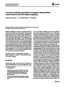
Location of the Sarcheshmeh mine and Shur River [27].

Artificial neural networks (ANNs) have gained increasing popularity in different fields of engineering in the past few decades because of their ability to extract complex and non-linear relationships. Hence, ANN has been widely used as reliable method for estimation and classification of the associated problems of heavy and toxic metals. In this way, estimation of the heavy metal concentration in soils has been applied using back propagation network and multiple linear regression [10]. The backpropagation neural network and multiple linear regression were used for prediction of water quality in the Gomti River (India) [11, 12]. However, in this paper, we will employ a reliable machine learning theory named support vector machine (SVM). Support vector machines, based on the structural risk minimization (SRM) principle [13], are a promising method for data mining and knowledge discovery. SVMs were introduced in the early 1990’s as a non-linear solution for classification and regression tasks [14]. The theory was based mainly on the consistency of a learning process, on how to control the generalization performance of a learning process [15]. There are at least three reasons for the continued success of SVM: its ability to learn well with only a very small number of parameters, its robustness against data error, and its computational efficiency compared with several other intelligent computational methods such as neural network, fuzzy network, etc. [16]. By minimizing the structural risk, SVMs work well not only in classification [17, 18] but also in regression [19, 20]. SVMs were soon introduced into many other research fields, e.g image analysis [21], signal processing [22] time series analysis [23] and they

usually outperformed the traditional statistical learning methods [24]. Thus, SVMs have been receiving more attention and are quickly becoming a very active research field. This study has been done with the aims of: 1) describing the process of nickel mobilization in mining waste dumps by introducing a novel conceptual model, and 2) predicting the nickel concentration using two algorithms, the support vector machine (SVM) and the general regression neural network (GRNN). Data collected from two sampling programs conducted on Shur River nearby the Sarcheshmeh copper mine, SE Iran will be used for both illustrating the pollution potential of this River and showing the strength of machine learning techniques in prediction of nickel mobilization.

2.

Material and Method

2.1.

Study area

Sarcheshmeh copper mine is located 160 km southwest of Kerman and 50 km southwest of Rafsanjan in Kerman province, Iran. The main access road to the study area is the Kerman- Rafsanjan-Shahr Babak road. This mine is located in the Band Mamazar-Pariz Mountains. The average elevation of the mine is 1600 m. The mean annual precipitation of the site varies from 300 to 550 mm. The temperature varies from +35◦ C in summer to −20◦ C in winter. The area is covered with snow for about 3 to 4 months per year. The wind speed can sometimes exceeds

376


R. Gholami, M. Ziaii, F. Doulati Ardejani, Sh. Maleki

to 100 km/h. Rough terrain is predominates around the mining area. Figure 1 shows the geographical position of the Sarcheshmeh copper mine. The orebody in Sarcheshmeh is roughly oval in shape, with a length of about 2300 m and a width of about 1200 m. This deposit is associated with the late Tertiary Sarcheshmeh granodiorite porphyry stock [25]. The porphyry is a member of a complex series of magmatically related intrusives emplaced in the Tertiary volcanics at a short distance from the edge of an older near-batholithsized granodiorite mass. An open pit mining method is used to extract copper at Sarcheshmeh. A total of 40,000 tons of ore (average grades 0.9% Cu and 0.03% Mo) is approximately extracted per day in Sarcheshmeh mine [26]. Because of the ineffective management of waste dump material, this mine site has a high potential for pollution generation and resulting hazardous problems.

2.2.

Figure 2.

Concept of ε-insensitivity. Only the samples out of the ±ε margin will have a non-zero slack variable, so they will be the only ones that will be part of the solution [30].

To estimate a linear regression f(x) = (w · x) + b

Sampling and field methods

Water sampling in the Shur River downstream from the Sarcheshmeh mine was conducted in February 2006. The samples consist of water from the Shur River (Figure 1) originating from Sarcheshmeh mine, acid leachates from the waste pile structure, run-off of leaching solution flowing into the River waters in direct contact with tailing. The water samples were immediately acidified by adding HNO3 (10 cc acid/1000 cc sample) and stored under cool conditions. The equipment used in this study was a sample container, GPS, oven, autoclave, pH meter, atomic adsorption and ICP analysers. The pH of the water was measured using a portable pH meter in the field. Other physical parameters measured include total dissolved solids (TDS), electrical conductivity (EC) and temperature. Analyses for dissolved metals were performed using atomic adsorption spectrometry (AA220) in the water Lab of the National Iranian Copper Industries Company (NICIC).

3.

Model Development

3.1.

Support Vector Machine

In pattern recognition, the SVM algorithm constructs nonlinear decision functions by training a classifier to perform a linear separation in some high dimensional space which is nonlinearly related to input space. To generalize the SVM algorithm for regression analysis, an analogue of the margin is constructed in the space of the target values (y) by using Vapnik’s ε-insensitive loss function 2 [28, 29]. |y − f(x)|ε := max {0, |y − f(x) − ε|}

(2)

Where w is the weighting matrix, x is the input vector and b is the bias term. With increasing precision, one minimizes m X 1 2 w +C |y − f(x)|ε (3) 2 i=1 Where C is a trade-off parameter to ensure the margin ε is maximized and error of the classification ξi is minimized. Considering a set of constraints, one may write the following relations as a constrained optimization problem: N

L(w, ξ, ξ 0 ) =

X 1 2 (ξi + ξi0 ) w +C 2 i=1

 T   yi − w · x − b ≤ ξi + ε Subject to : yi + w T · x + b ≤ ξi0 + ε   ξi , ξi0 , xi ≥ 0

(4)

(5) (6) (7)

According to relations 5 and 6, any error smaller than ε does not require a nonzero ξi orξi0 , and does not enter the objective function 4 [31]. By introducing Lagrange multipliers (α and α 0 ) and allowing for C > 0, ε > 0 chosen a priori, the equation of an optimum hyper plane is achieved by maximizing the following relations: L(α, α 0 ) = N N N X 1 XX (αi − αi0 )xi0 xi (αi − αi0 ) + ((αi − αi0 )yi − (αi + αi0 )ε) 2 i=1 i=1 i=1

(1)

(8) 377



Table 1.

Polynomial, normalized polynomial and Radial Basis Function (Gaussian) Kernels [34].

Kernel Function

Type of Classifier

K (xi , xj ) = (xiT xj + 1)ρ

Complete polynomial of degree ρ

K (xi , xj ) =

(xiT xj +1)ρ

q

Normalized polynomial kernel of degree ρ

(xiT xj )−(yTi yj )

i h

2 K (xi , xj ) = exp xi − xj /2σ 2

Subject to 0 ≤ (αi − αi0 ) ≤ C

Gaussian (RBF) kernel with parameter σ which controls the half-width of the Curie fitting peak

(9)

Where, xi only appears inside an inner product. To get a better potential representation of the data in the nonlinearized case, the data points can be mapped into an alternative space, generally called feature space (a preHilbert or inner product space) through a replacement: xi xj → φ(xi )φ(xj )

N X N X

(αi − αi0 )φ(xi )T φ(xj ) + b

i=1 j=1 N X N X

=

(αi − αi0 )K (xi , xj ) + b

(11)

i=1 j=1

Where b is computed using the fact that equation 5 becomes an equality with xi = 0 if 0 < αi < C, and relation 6 0 becomes an equality withxi = 0 if 0 < αi0 < C [35, 36].

3.2.

3.3.

Building an optimal SVM

(10)

The functional form of the mapping φ(xi ) does not need to be known since it is implicitly defined by the choice of kernel: k(xi ,xj ) = φ(xi )· φ(xj ) or inner product in Hilbert space. With a suitable choice of kernel the data can become separable in feature space while the original input space is still non-linear. Thus, whereas data for n-parity or the two spirals problem is non-separable by a hyper plane in input space, it can be separated in the feature space by the appropriate kernels [32, 33]. Table 1 gives some of the common kernels. Then, the nonlinear regression estimate takes the following form: yi =

the requirements of the computation algorithms, the data of both the input and output variables were normalised to an interval by transformation process. In addition, the leave-one-out (LOO) cross-validation of the whole training set was used for adjusting the associated parameters of the network[37].

Data Set

One of the main objectives of this study is to predict nickel concentration from AMD by incorporating the samples collected from the Shur River near the Sarcheshmeh copper mine. As a matter of fact, physical and chemical constitutions are considered as inputs, whereas nickel concentration is taken as the output of the networks. In view of

Similar to other multivariate statistical models, the performance of the SVM for regression depends on the combination of several parameters. They are the capacity parameter C, ε of the ε-insensitive loss function, and the kernel type K and its corresponding parameters. C is a regularization parameter that controls the trade-off between maximizing the margin and minimizing the training error. If C is too small then insufficient stress will be placed on fitting the training data. If C is too large then the algorithm will overfit the training data. But, Wang et al., (2003) indicated that the prediction error was scarcely influenced by C. In order to make the learning process stable, a large value should be set up for C (e.g., C = 100). The optimal value for ε depends on the type of noise present in the data, which is usually unknown. Even if enough knowledge of the noise is available to select an optimal value for ε, there is the practical consideration of the number of resulting support vectors. ε-insensitivity prevents the entire training set meeting boundary conditions, and so allows for the possibility of sparsity in the dual formulations solution. So, choosing the appropriate value of ε is critical. Since in this study the nonlinear SVM is applied, it is necessary to select a suitable kernel function. The obtained results of published research work[38, 39] indicate that the Gaussian radial basis function has a superior efficiency than other Kernel functions. As seen in Table 1, Gaussian kernel is as follows:

378


K (xi , xj ) = e−|xi −xj |

2

/2σ 2

(12)


Where σ is a constant parameter of the kernel controlling the amplitude of the Gaussian function and the generalization ability of the SVM. We have to optimize σ . In order to find the optimum values of the two parameters (σ and ε) and prohibit the overfitting of the model, the data set was separated into a training set of 40 compounds and a test set of 26 compounds randomly (i.e. MATLAB multi-purpose commercial software was used for implementing the automated Bayesian regularization process of random selection) and a leave-one-out cross-validation of the whole training set was performed. The leave-one-out (LOO) procedure consists of removing one example from the training set, constructing the decision function on the basis only of the remaining training data and then testing on the removed example [37]. In this way one can test all examples of the training data and measure the fraction of errors over the total number of training examples. The root mean square error (RMSE) was used as an error function to evaluate the quality of the model. The detailed process of selecting the parameters and the effects of every parameter on the generalization performance of the corresponding model are shown in Figure 3. To obtain the optimal value of σ , the SVM with different σs was trained, the σ varying by 0.01 over an interval of 0.01 to 0.3. We calculated the RMS on different σs , according to the generalization ability of the model based on the LOO cross-validation for the training set in order to determine the optimal value. The curve of RMSE versus sigma is shown in Figure 3. The optimal σ was 0.16. In order to find an optimal ε, the RMSEs for different εs were calculated. The curve of the RMSE versus epsilon is also shown in Figure 3. From Figure 3, the optimal ε was found as 0.08. From the above discussion, the σ , ε and C were fixed to 0.16, 0.08 and 100, respectively, when the support vector number of the SVM model was 41. Figure 4 is a schematic diagram showing the construction of the SVM. When finding the most relevant input variables for predicting the nickel concentration in water among many combinations of attributes (different physical and chemical parameters), the best input was selected by a trial and error method (Table 2). Two criteria were used in order to evaluate the effectiveness of the network and its ability to make accurate predictions. The Root mean square error (RMSE) can be calculated as follows: r Pn RMSE =

i=1 (yi

n

Figure 3.

Sigma versus RMS error (left) and Epsilon versus RMS error (right) on LOO cross-validation.

Figure 4.

Schematic diagram of optimum SVM for prediction of nickel concentration.

ˆ i )2 −y (13)

ˆ i denotes the predicted Where, yi is the measured value, y value, and n stands for the number of samples. RMSE indicates the discrepancy between the measured and predicted values. The lower the RMSE, the more accurate

379



Table 2.

Correlation coefficient (R) and RMS of the prediction based on different input variables.

Input variables

R (Train) R(Test) RMSE (Train) RMSE (Test)

pH, SO4 , HCO3

0.910

0.78

0.34

0.46

pH, SO4 , HCO3 , TDS, EC

0.935

0.81

0.27

0.36

pH, SO4 , HCO3 , TDS, EC, Mg

0.955

0.87

0.22

0.29

0.98

0.94

0. 12

0.21

pH, SO4 , HCO3 , TDS, EC, Mg, Fe, Zn, Cu

the prediction is. The efficiency criterion, R, is given by: v Pn u u ˆ i )2 (yi − y R = t1 − P i=1 Pn ˆ 2i n 2 i=1 y i=1 yi − n

(14)

Where R, the efficiency criterion, represents the percentage of the initial uncertainty explained by the model. The best fit between measured and predicted values, which is unlikely to occur, would be RMSE=0 and R=1. It was found that a combination of nine parameters (pH, SO4 , HCO3 , TDS, EC, Mg, Fe, Zn, and Cu) is the most suitable input variable set. In fact, these nine parameters are thought to play an important role in nickel mobilization in water. Table 2 gives the correlation coefficient (R) and RMSE of the prediction based on different input variables. The optimum SVM was then used to predict concentrations of nickel in the collected water samples from the Shur River near the Sarcheshmeh copper mine. The results of these analyses are discussed below.

4.

Results

4.1.

Conceptual model of nickel mobilization

Conceptual modeling is the process of formally documenting a problem domain for the purpose of understanding and communicating the relationships between major parameters [40]. Generally, conceptual models can be used to support the development, acquisition, adaptation, standardization and integration of information systems [41]. As a rule, an effective conceptual model must (1) be expressive enough to distinguish among different data types, relationships, and constraints; (2) be simple to understand; (3) have minimal, distinct and orthogonal basic concepts, which should be formally defined; and (4) have a single systematic interpretation [42]. Therefore, designing an appropriate conceptual model for nickel mobilization due to sulphide-bearing mineral oxidation in natural systems provides an opportunity to evaluate the equations of the system and perhaps give useful information for designing

Figure 5.

Conceptual model of nickel mobilization.

a suitable remediation strategy. Figure 5 gives a conceptual model design based on the results obtained from the sampling program. This model addresses the most crucial mechanisms of the nickel mobilization process, which are oxygen diffusion, chemical reactions, and the transport of oxidation products through water. The model assumes that the backfilled materials consist of spherical, uniformly sized particles surrounded by a water film. Particles are assumed to have a homogeneous distribution of pyrite grains within them. Oxidation reactions and products diffuse through the particle between the pyrite grains and the spoil solution surrounding the particles. Pyrite oxidation occurs at the surface of the pyrite grains contained within the particles. Oxygen diffuses from zones of higher oxygen concentration to zones of lower oxygen concentration through the air-filled pore space in the backfilled materials, with the oxygen in equilibrium with the spoil solution. It was assumed that diffusion is the dominant process supplying oxygen for oxidation reactions. Complexation of ferric iron is also assumed to take place within the solution. A reaction between H+ in solution and the spoil matrix can occur, consuming H+ from the spoil solution and increasing the pH. Equilibrium-controlled ion exchange is assumed to take place between the solution and solid phases within the spoil solution. It is assumed that ions of Fe2+ partici-

380



Table 3.

Maximum, minimum and mean physical and chemical constituents including toxic metals from water samples from the Shur River (concentrations of elements are given in ppm). 2+ Mg2+ pH SO2− HCO− 4 3 Ca

Min

3.3

27

Max 7.20 1526

Cu

0

92

13

0

628

460

123

158

Mn

Zn

TDS

0.02 0.01 0.04

Ni

0

446

25

Fe

23

52

31.48 2080.68

Mean 5.27 778.45 34.01 182.78 56.70 20.29 4.5 4.60 16.05 6.33 1009.90

EC (µS/cm) 870 2260 1306.52

pate in the ion exchange reaction, precipitation Fe(OH)3 , which removes Fe3+ and releases H+ into the solution. The oxidation products (i.e. Nickel, etc) are transported through water flow system under low pH conditions. Any increase in pH decreases the solubility of the nickel in aqueous phase and transfers it to solid phase. In this model, chemical oxidation of Fe2+ , pyrite oxidation by oxygen and ferric iron, and oxygen diffusion, are relatively slow but ion exchange and complexation reactions as well as precipitation reactions are fast and assumed to be equilibrium controlled reactions. The above discussion about the condition of nickel mobilization can be completely verified using the obtained results of sampling program described in material and method section. Table 3 gives the associated results of this sampling program. As it is seen in Table 3, concentrations of nickel and other heavy metals (i.e. Fe, Cu, and Zn) are considerably high. Moreover, the pH is low and a considerable amount of SO−2 4 were produced confirming that contamination from sulfide-mineral oxidation has impacted these samples. These data were considered a good test case for our model for nickel mobilization in mining site areas.

4.2. Prediction of nickel concentration using SVM and GRNN As described in Section 3, we built an efficient SVM for prediction the concentration of nickel. In this section, we are going to present the obtained results of SVM by comparing the predicted values of nickel with measured ones. Figure 6 shows the performed work of SVM in the test dataset. As shown in Figure 6, there is acceptable agreement (correlation coefficient of 0.94) between the predicted and measured values of nickel. However, for showing the strength of the SVM in providing an accurate prediction, performance of this machine learning methodology is compared with that of a general regression neural network (GRNN) (Figure 7). GRNN is a one-pass learning algorithm with a highly parallel structure. This method is a modification to the probabilistic neural network that has been successfully used in

Figure 6.

Relationship between the measured and predicted nickel produced by SVM (left) and estimation capability of SVM (right).

many engineering applications. Huang and Williamson (1994) described GRNN as an easy-to-implement tool that has efficient training capabilities and the ability to handle incomplete patterns. GRNN is known to be particularly useful in approximating continuous functions [43]. To assess the capabilities of this machine learning methodology, there was an attempt to construct a proper GRNN for prediction of nickel concentration. The GRNN constructed for this study was a multi-layer neural network with one hidden layer of radial basis function consisting 18 neurons and an output layer containing only one neuron. Multiple layers of neurons with nonlinear transfer functions allow the network to learn nonlinear and linear relationships between the input and output vectors. Figure 7 shows the prediction performance for this network. As depicted in Figure 7, GRNN-predicted versus measured nickel concentrations are only marginally less accurate than those of the SVM. Therefore, this network can be considered as another suitable method for toxic metal concentration prediction. An additional verification step outlined in the next section can provide a better insight into this statement.

4.3.

Verification

Verification and comparisons of the strengths of the SVM and GRNN in predicting nickel concentration was con381



Table 4.

Comparisons of the performance of each network based on their RMSE.

SVM

Input variables

GRNN

R (Train)

R (Test)

RMSE (Train)

RMSE (Test)

R (Train)

R (Test)

RMSE (Train)

RMSE (Test)

0.98

0.94

0.12

0.21

0.98

0.90

0.12

0.42

pH, SO4 , HCO3 , TDS, EC, Mg, Fe, Zn, Cu

5.

Figure 7.

Relationship between the measured and predicted nickel produced by GRNN (left) and estimation capability of GRNN (right).

Figure 8.

Performance of the SVM and GRNN in prediction of nickel data from Doulati et al. (2008).

Conclusions

In this paper we have investigated the nickel mobilization process in mine waste dumps. We have designed a novel conceptual model describing the mechanism of nickel generation and mobilization in water flow system. In addition, support vector machine (SVM) is a novel machine learning methodology based on statistical learning theory (SLT), which results in a uniquely global optimum, high generalization performance, and prevention from converging to a local optimal solution. In this study, in addition to discussing the most important parameters related to the nickel mobilization, we have shown the application of machine learning methodologies for predicting nickel concentration in the Shur River near the Sarcheshmeh copper mine. The results show that SVM can predict the nickel concentration marginally better than the general regression neural network (GRNN) and both of them can be considered as valuable tools for toxic metal concentration prediction. The results of this study are important for environmental scientists as they can help to deal with the condition of nickel mobilization and its related parameters appropriately.

Acknowledgements Authors greatly appreciate anonymous reviewers and Dr W. Mayes for his constructive comment and contribution in helping to improve the manuscript.

ducted using a sampling program previously conducted on the Shur River. This sampling program is documented in Doulati et al. (2008). Ten samples containing different concentrations of nickel were used for verification purposes. Results are shown in Figure 8. As shown in Figure 8, SVM prediction is only marginally better than that of the GRNN. Table 4 shows the RMSE for each network prediction. Table 4 shows that both of these methods are robust tools for predicting toxic metal concentrations in water. However, in terms of running time, the SVM performed the prediction considerably faster than the GRNN.

References [1] Trois C., Marcello A., Pretti S., Trois P., Ross G.I., The environmental risk posed by small dumps of complex arsenic, antimony, nickel and cobalt sulphides. J. Geochem. Explor., 2007, 92, 83–95 [2] Walder I.F., Schuster P.P., Mine Waste Management in Proceedings of Environmental Geochemistry of ore deposits and mining activities, Presented by SARB Consulting in Oslo, Norway, May 1997

382



[3] Romero A., Gonzalez I., Galan E., Estimation of potential pollution of waste mining dumps at Pena del Hierro (Pyrite Belt, SW Spain) as a base for future mitigation actions. Appl. Geochem., 2006, 21, 1093– 1108 [4] Legge 319 (Merli) del 10.05.1976 pubblicata nella Gazzetta Ufficiale N. 141 del 29.05.1976 [5] Emendamento della Legge 319 (Merli) del 10.05.1976 pubblicata nella Gazzetta Ufficiale N. 141 del 29.05.1976, Regione Autonoma della Sardegna., 1983 [6] Mayes W.M., Johnston D., Potter H.A.B., Jarvis A.P., A national strategy for identification, prioritisation and management of pollution from abandoned noncoal mine sites in England and Wales. Methodology development and initial results. Sci. Total Environ., 2009, 407, 5435-5447 [7] Amezaga J., Rotting T.S., Younger P.L., Nairn R.W. Noles A.J., Oyarzun R., Quintanilla J., A rich vein? Mining and the pursuit of sustainable development. Environ. Sci. Technol., 2011, 45, 21-26 [8] Alvarez E., Fernandez Marcos M.L., Vaamonde C., Fernandez-Sanjurjo M.J., Heavy metals in the dump of an abandoned mine in Galicia (NW Spain) and in the spontaneously occurring vegetation. Sci. Total Environ., 2003, 313, 185–197 [9] Accornero M., Marini L., Ottonello G., Zuccolini M.V., The fate of major constituents and chromium and other trace elements when acid waters from the derelict Libiola Mine (Italy) are mixed with stream waters. Appl. Geochem., 2005, 20, 1368-1390 [10] Kemper T„ Sommer S., Estimate of Heavy Metal Contamination in Soils after a Mining Accident Using Reflectance Spectroscopy. Environ. Sci. Technol., 2002, 36, 2742-2747 [11] Khandelwal M., Singh T.N., Prediction of mine water quality by physical parameters. J. Sci. Ind. Res., 2005, 64, 564-570 [12] Singh K.P., Basant A., Malik A., Jain G., Artificial neural network modeling of the river water quality a case study. Ecol. Model., 2009, 220, 888-895 [13] Stitson M., Gammerman A., Vapnik V., Vovk V., Watkins C., Weston J., Advances in Kernel Methods - Support Vector Learning. MIT Press, Cambridge, 1999 [14] Behzad M., Asghari K., Morteza E., Palhang M., Generalization performance of support vector machines and neural networks in run off modeling. Expert Syst. Appl., 2009, 36, 7624–7629 [15] Cortes C., Prediction of generalization ability in learning machines. PhD thesis, University of Rochester, USA, 1995 [16] Wang L., Support Vector Machines: Theory and Ap-

[17]

[18]

[19]

[20]

[21]

[22]

[23]

[24]

[25]

[26]

[27]

[28]

[29]

[30]

[31]

plications. Springer Berlin Heidelberg, New York, 2005 Zhou D., Xiao B., Zhou H., Global geometric of SVM classifiers. Technical Report, Institute of Automation, Chinese Academy of Sciences, 2002 Bennett K.P., Bredensteiner E.J., Geometry in Learning, Geometry at Work, Mathematical Association of America, Washington, DC, 1998 Mukherjee S., Osuna E., Girosi F., Nonlinear prediction of chaotic time series using a support vector machine. In: Proceedings of the 1997 IEEE Workshop, Amelia Island, 1997, 511–520 Jeng J.T., Chuang C.C., Su S.F., Support vector interval regression networks for interval regression analysis. Fuzzy Set System, 2003, 138, 283–300 Seo, K.K., An application of one-class support vector machines in content based image retrieval. Expert Syst. Appl., 2007, 33, 491–498 Widodo A., Yang B. S., Wavelet support vector machine for induction machine fault diagnosis based on transient current signal. Expert Syst. Appl., 2008, 35, 307–316 Francis E.H., Tay L.J., Modified support vector machines in financial time series forecasting. Neurocomputing, 2002, 48, 847–861 Steinwart I., Support Vector Machines. Los Alamos National Laboratory, Information Sciences Group (CCS-3), Springer, 2008 Banisi S, Finch JA., Testing a floatation column at the Sarcheshmeh copper mine. Mineral Engineering, 2001, 14, 785-789 Shahabpour J., Doorandish M., Mine drainage water from the Sarcheshmeh porphyry copper mine, Kerman, IR Iran. Environment Monitoring and Assessment, 2008, 141, 105–120 Derakhshandeh R., Alipour M., Remediation of Acid Mine Drainage by using Tailings Decant Water as a Neeutralization Agent in Sarcheshmeh Copper Mine. Research Journal of Environmental Sciences, 2010, 4, 250-260 Quang-Anh T., Xing L., Haixin D., Efficient performance estimate for one-class support vector machine. Pattern Recogn. Lett., 2005, 26, 1174–1182 Stefano M., Giuseppe J., Terminated Ramp–Support Vector Machines: A nonparametric data dependent kernel. Neural Networks, 2006, 19, 1597–1611 Liu H„ Wen S., Li W., Xu C., Hu C., Study on Identification of Oil/Gas and Water Zones in Geological Logging Base on Support-Vector Machine. Fuzzy Information and Engineering, 2009, 2, 849–857 Lia Q., Licheng J., Yingjuan H., Adaptive simplification of solution for support vector machine. Pattern

383



Recognition, 2007, 40, 972–980 [32] Scholkopf B., Smola A.J., Muller K.R., Nonlinear component analysis as a kernel eigenvalues problem. Neural Computing, 1998, 10, 1299–1319 [33] Walczack B., Massart D.L., The radial basis functions—partial least squares approach as a flexible non-linear regression technique. Analitica Chimica Acta, 1996, 331, 177–185 [34] Wang L., Support Vector Machines: Theory and Applications. Springer Berlin Heidelberg New York, 2005 [35] Chih-Hung W., Gwo-Hshiung T., Rong-Ho L., A Novel hybrid genetic algorithm for kernel function and parameter optimization in support vector regression. Expert Syst. Appl., 2009, 36, 4725–4735 [36] Sanchez D.V., Advanced support vector machines and kernel methods. Neurocomputing, 2003, 55, 5–20 [37] Liu H., Yao X., Zhang R., Liu M., Hu Z., Fan B., The accurate QSPR models to predict the bioconcentration factors of nonionic organic compounds based on the heuristic method and support vector machine. Chemosphere, 2006, 63, 722–733 [38] Dibike Y.B., Velickov S., Solomatine D., Abbott M.B., Model Induction with support vector machines: Introduction and Application. J. Comput. Civil Eng., 2001, 15, 208–216 [39] Han D., Cluckie I. Support vector machines identification for runoff modeling. In: Liong S.Y., Phoon K.K., Babovic V. (Eds.), Proceedings of the sixth international conference on hydroinformatics, June, Singapore, 2004, 21–24 [40] Maier R., Organizational concepts and measures

[41]

[42]

[43]

[44]

[45]

[46]

for the evaluation of data modeling. In: Becker S. (Ed.), Developing Quality Complex Database Systems: Practices, Techniques and Technologies, Idea Group Publishing, Hershey, USA, 2001, 1–27 Motschnig-Pitrik R., The semantics of parts versus aggregates in data/knowledge modeling. Lect. Notes in Comput. Sc., 1993, 685, 352–373 Borgida A., Knowledge representation, semantic modeling: similarities and differences. In: Kangasalo H. (Ed.), Entity–Relationship Approach: The Core of Conceptual Modeling. Elsevier Science Publishers, 1991 Artun E., Mohaghegh S., Toro J., Reservoir Characterization Using Intelligent Seismic Inversion. The Society of Petroleum Engineers Eastern Regional Meeting, Morgantown, West Virginia, 14–16 September 2005, Wang W.J., Xu Z.B., Lu W.Z., Zhang X.Y., Determination of the spread parameter in the Gaussian kernel for classification and regression. Neurocomputing, 2003, 55, 643–663 Huang Z., Shimeld J., Williamson M., Katsube J., Permeability prediction with artificial neural network modeling in the Venture gas field, offshore eastern Canada. Geophysics, 1996, 61, 422-436 Doulati Ardejani F., Karami G.H., Bani Assadi A., Atash Dehghan R. Hydrogeochemical investigations of the Shour River and groundwater affected by acid mine drainage in Sarcheshmeh porphyry copper mine. 10th International Mine Water Association Congress, 2-5 June 2008, Karlovy Vary, Czech Republic, 2008, 235-238

384
