http://archive.csa.iisc.ernet.in/TR/2006/3/. Computer Science and .... An application programming interface (API) can also be looked at as a reac- tive system.
Specification Based Regression Testing Using Explicit State Space Enumeration Sujit Kumar Chakrabarti
Y. N. Srikant
IISc-CSA-TR-2006-3 http://archive.csa.iisc.ernet.in/TR/2006/3/
Computer Science and Automation Indian Institute of Science, India April 2006
Specification Based Regression Testing Using Explicit State Space Enumeration Sujit Kumar Chakrabarti
Y. N. Srikant
Abstract When a software system enters maintenance phase, Regression Testing becomes an important Software Engineering activity. Large size and complex nature of the software, frequent releases and low defect rate demands in subsequent releases and patches makes it imperative to carry out regression testing in a near exhaustive and efficient manner. This paper presents a method of partial automation of specification based regression testing, ESSE (Explicit State Space Enumeration). The central idea of ESSE method is the extraction of a finite state model of the system making use of an already tested version of the system under test. We demonstrate the usefulness of the finite state model thus obtained by presenting two new algorithms for test sequence computation – both based on our finite state model generated by the above method. We also provide the details and results of the experimental evaluation of ESSE method. Comparison with a practically used random-testing algorithm has shown substantial improvements.
1 1.1
Introduction State Space Representation of a Program
A program can be approximated by a finite state model. The concept of modelling a program by a finite state automaton is there for a long time. Such a model, if it exists, can be fruitfully used as a software engineering aid in a variety of ways. For instance, in model-checking, a finite state model, called the labeled transition system (LTS), is used to represent the system to be verified. Similary, there is a whole body of literature that demonstrates the use of finite state models for automatic generation of test-data. 1
Start L1
x←0 L2
x 6= 100
no
Stop
? L3
yes
L4
x←x+1
Figure 1: An example program. However, the major body of works in verification (model-checking), and model-based testing, presuppose the existence of a finite state model. However, this is not always the case. Due to the dearth of a finite state model of the system, it becomes difficult to put many powerful test automations into practice. In this work we present an algorithm which reverse-engineers a finite state model of a system. We then demonstrate the usefulness of such a model with an elaborate example of its application in the area of specification based software regression testing, and with a brief example of its application in software verification.
1.2
Examples
A computer program may be thought of as a state based system. What is considered to represent its state can vary from case to case, primarily depending upon the purpose of modelling. For example, consider the program in figure 1 There are more than one ways of modelling the system shown in figure 1 as a finite state machine. For instance, considering each program point as a state can be one way. That will give us the transition system as shown in figure 2. Another way of finite state modelling of the same program is by considering each value of variable x as a state. then the program will be represented by a model shown in fig 3. Yet another model would be to consider intervals of values taken up by x as individual states. for example, if we partition the domain of x in the 2
x←0
x = 100
L1
L2
L4 !(x = 100)
x←x+1 L3
Figure 2: Finite state model with program points as states. x=0
x = 99
x=1
x = 100
Figure 3: Finite state model with individual values of x as states. following manner: (0, 9), (10, 19), ... (90, 99), (100, 109) ... Then we get another finite state model as shown in figure 4. If we model the system by the values of another abstract state variable y such that y = x%3, then we get the state machine as shown in figure 5. The purpose behind citing many such examples was to clarify that for a single given system there could be arbitrarily many ways of creating a finite state model of that system. Which one is actually selected is dependent on the purpose of modelling. In the program analysis community, the finite state model of choice is the control flow graph which implicitly models each basic-block boundary as a state, as in figure 1 and figure 2. Model checing community prefers labeltransition system as the finite state model of choice, as described in the rest of the examples. In testing community both control-flow graph and labelled transition systems are of interest, primarily because testing researchers adapt methods and techniques of both model checking and program analysis for automating test data generation. As in the case of all modelling, finite state modelling of a program involves abstracting out the relevant details while leaving out the rest. A model’s usefulness as an object of analysis rests on its being simpler in some appropriate way than the system it models. Simplification and reduction in model size are, therefore, two prime objectives of modelling. For example, when in the above example the program is modelled as s1
s10
s2
s11
Figure 4: Finite state model with intervals of values of x as states. 3
y=1 and x = 100
y=0
y=1
y=2
Figure 5: Finite state model with y = x % 3 as states. CFG, we are modelling the program points as the state-variable. In a reallife implementation a program point is essentially nothing but the value of the program counter(PC). In reality, however, the target machine implementation of any program would naturally contain many more program points – and hence distinct values of the machine program counter – than are explicit in the example program. However, many of those PC values are of little interest in most problems of program analysis. The CFG model created in practice would generally appear as it is shown, and not any more elaborate. Similarly, in the remaining examples, a model explicitly models each individual values that the variable x takes; and ends up having 101 states. Another model models states in terms of continuous intervals of 10 values each, resulting in a reduced state space of 11 states. Modelling the same program by each state representing a distinct value of x%y results in an even further reduced state-space of 4 states. Economy of the resultant model on the one hand, and the fine-grainedness of the information content on the other, are the two main factors that have to be considered while choosing an appropriate level of abstraction in the model.
1.3
Reactive Systems and Finite Modelling
A large body of softwares today can be put into the class of reactive systems. Reactive systems are systems which do not run from start to end on being invoked, in the manner a compiler does. Instead, such a system waits (potentially endlessly) for inputs from the user or the environment, and carries out some computation in response to that. GUI applications, embedded applications, web-server applications, operating systems etc. are some typical examples of reactive systems. Finite state modelling is popular in thinking about reactive systems. Hence, they have been used extensively in design (UML statechart and its
4
variants), verification and validation of such systems.
1.4
An Example of A Reactive System – An Application Programming Interface
An application programming interface (API) can also be looked at as a reactive system. The API functions are the ways by which input events can be sent to the API. Consider the complete program shown in figure 6. The contents of the two files PUT.h and PUT.cpp constitute a very trivial API program. An external code can link to this code (PUT.cpp could be compiled beforehand and be provided as a library), and make calls to the API functions. A possible stub making a sequence of calls to PUT API is as shown in figure 7. Together with main we have created a trace that PUT API can traverse through. This would be a substring of some valid run through the automaton that models the PUT API. If we model PUT by representing each value of x as a state of the statespace graph, it would appear as shown in figure 8.
1.5
Problem Context
In the above example, x is the state-variable whose value is determining the state. In lines similar to that described in the last section, some other statevariable could have been chosen. It would have given us another state-space model of the system. The choice of the state-variable, and hence the state space model, depends on the specific requirement of modelling. In our present context, the purpose of modelling is testing. In a typical scenario of software maintenance, a large API is used by many groups within an industrial software development firm. A dedicated group is continuously involved in all kinds of maintenance activities upon this API library – bug fixing, enhancement (both feature and performance), and preventive. Thus, new minor releases arrive quite frequently. Before the new patch can be integrated with all client modules, extensive regression testing is necessary. Due to the nature and scale of the software, this regression testing is done as a black-box testing, possibly by yet another team of testers having no access to the source code of the API library. The above process is diagrammatically represented in figure 9. The process shown in figure 9 is endlessly cyclic. Moreover, it is constrained by tight release-cycles. The testing team, more than any other team, is under strong pressure to carry out the regression testing as efficiently as
5
////////// PUT .h ////////////////// # ifndef PUT_H # define PUT_H int get_x (); void set_x ( const int ); void f1 (); void f2 ( const int , const int ); void reset (); # endif
////////// PUT . cpp ////////////////// # include < iostream > # include " PUT .h" using namespace std ; static int x = -10; int get_x ()
{
return x ;
}
void f1 ()
{
x ++;
}
void f2 ()
{
x += 2;
}
void f3 ()
{
x += 10;
}
void reset ()
{
x = -10;
}
Figure 6: An example of an API
6
// main . cpp # include " PUT . cpp " int main () { f1 (); f1 (); f2 (); f1 (); f3 ();
// // // // // //
x x x x x x
== == == == == ==
-10 -9 -8 -6 -5 5
return 0; }
Figure 7: A stub for creating a trace from the state-space of the program in figure 6
f2 f1
f2
f3
x > 10 f3
x = −10
f3
x = 10 f3
f1 f3
x = −9
f2
-10 ≤ x ≤ -5
f2
f3
x=9 f3
f1
f1
x = −8
x=8
f1
f1
x = −7
f2
f1 f2
f2 f3
f2
f2
5 ≤ x ≤ 10
x=7 f3
f1
f1
x = −6
x=6
f2 f3
f1 f3
-5 < x < 5
x = −5
f1 f2
f2
f1
x=5
f3
f1
Figure 8: Explicit state space of the program in figure 6
7
API Provider
API Library
Testing Team
User 1..n
update
not satisfactory
provide regression test
test done report verdict
satisfactory release
Figure 9: Regression testing process possible with as little loss in completeness as possible. In short, automatic methods of carrying out specification based regression testing are of great importance to the testing team in a setup of this kind.
1.6
Contributions
In this direction this work contributes by providing a specification based regression-testing method. We have implemented our central idea in a prototype tool named ‘Modest’ (Model-Based Tester). The main contributions of this research work are: 1. An algorithm, called GraphMaker, to generate a finite state-space model of an API library, as described in the last section. 2. Demonstration of the application of such a model in test sequence computation by integration with many new algorithms and existing tools for computation of efficient test sequences. 3. Experimental evaluation of ESSE approach in comparison with an industrially used variant of random-testing, called legal random call approach throwing light on the performance of both methods.
8
1
1 7
2
3
5 4
7
2
3 6
5 4
(a)
6 (b)
Figure 10: Example of a DFS strand
2
GraphMaker
GraphMaker is an algorithm which generates a state space model of an API system by explicitly exploring the bounds. The GraphMaker algorithm is essentially an adaptation of the preorder depth first search (DFS) algorithm. The fundamental difference is, of course, that there is no graph to traverse when the algorithm starts executing. Nodes are created as GraphMaker traverses them. The order in which the nodes of a graph are created is the same as that in which the nodes of a digraph get marked in a preorder DFS.
2.1
GraphMaker-DFS, The DFS version of GraphMaker
As mentioned above, the GraphMaker algorithm is a preorder DFS algorithm. The basic ideas are as follows. To understand the GraphMaker in its core, just consider a simpliflied version of it – a depth first traversal algorithm without backtracking which we call GraphMaker-DFS. These essentials carry over fully to GraphMaker, the algorithm for the creation of the state space graph, with some minor additions. 2.1.1
DFS Strand
The operational difference between GraphMaker-DFS and preorder DFS is that GraphMaker-DFS cannot literally backtrack. Consider the graph shown in figure 10. The order in which a preorder DFS would traverse this graph is: 1, 2, 3, 4, 5, 6, 7. Same would be the order in which GraphMaker would create the nodes while making the graph. However, the traversal order of GraphMaker-DFS is as follows: 1, 2, 3, 4, 3, reset, 1, 2, 5, 4, reset, 1, 2, 5, 6, reset, 1, 2, 5, 7, 1, reset, 1, 2, 7, reset.
9
The underlined node identifiers denote that that node is being visited for the first time. Observe that each time the preorder DFS backtracks, GraphMaker-DFS resets, i.e. it goes all the way back to the initial state. It then traces its way back to the node the backtracking would have taken it to, and proceeds as the preorder DFS. We call each portion of the node traversal sequence of GraphMaker-DFS between two consecutive resets as a DFS strand. Formally, a DFS strand is a portion of the DFS traversal that results from a traversal starting at the root node and going on till it can. For example, figure 10 shows two DFS strands through the edges drawn in bold: in (a) it is 1, 2, 3, 4; and in (b), it is 1, 2, 5, 4. The conditions of termination of a DFS strand are the same as those for backtracking in DFS, that is: 1. Encountering a leaf 2. Encoutering an already visited node In both the above cases GraphMaker calls reset(), causing a return to the initial state. Each DFS strand has two phases. The former phase, phase 1, constitutes of a traversal through 0 or more already created nodes (and edges) to a node that would have been the destination of a backtrack in a proper preorder DFS. The latter phase, phase 2, is constituted of traversal through 1 or more untraversed edges, and 0 or more uncreated nodes of the state-space graph. Please note that traversal through already traversed edges and already created nodes is always contiguous in the phase 1 of a DFS strand. There cannot be traversed any already traversed edge or already created node once the DFS strand has terminated phase 1 and entered the phase 2. In fact, a DFS strand terminates if it encouters an already created node, as mentioned in (2) of the termination conditions of a DFS strand above. 2.1.2
LastFork
The ‘backtracking’ feature of DFS is simulated in GraphMaker-DFS by resetting the system and returning to the destination of the backtracking step from the root of the state space graph. We call this node the LastFork in GraphMaker-DFS. It is the lowest node in the current DFS strand which has untraversed outgoing edges. In figure 11, we have shown two snapshots of the process of graphmaking in a typical run of GraphMaker. In both (a) and (b), the nodes and edges drawn in bold indicate the current DFS strand. The bottommost node in this DFS strand is the most recently touched node. The shaded node (2 10
1
1 7
2
3
5 4
7
2
3 6
5 4
(a)
6 (b)
Figure 11: Example of a LastFork in (a) and 5 in (b)) are the LastForks in the respective snapshots. Precise characteristics of a LastFork node are as follows: 1. It is a member of the current DFS strand. 2. It has got atleast one outgoing edge which has yet not been traversed. 3. If it (i.e., say l, labelled LastFork) is above the node currently being traversed, say n, there should not be another node, say l 0 , in the current DFS strand such that the path p ∈(current DFS strand) joining l with n, contains l0 . If l is after n in the DFS strand, then in the last DFS strand, say DF SS 0 , there should not be another node l 0 ∈ DF SS 0 , such that the number of outgoing edges from l 0 is not equal to 0, and there exists a path p ∈ DF SS 0 from l to l0 . 4. All edges and nodes covered after encountering the LastFork in the current DFS strand have been created in this strand itself. This is a direct corollary of the basic definition of the LastFork. 2.1.3
PrevFork
During the traversal of DFS strand, the LastFork mark may shift both downward or upward. The downward shift happens when, after crossing the present LastFork node l, the DFS strand encouters (by creating) a new node, l0 , with atleast 2 outgoing edges. On this, l 0 becomes the LastFork. Another mark name PrevFork is associated with l. Upward shift of the LastFork mark happens when during the traversal, all the outgoing edges of current LastFork node get traversed. The LastFork mark then is shifted to the node marked PrevFork. 11
1
1
1 2
6
2 3
4
5
4
5
2
3
3
6
4 5 6
(a)
(b)
1
1
(c) 1
2
2 3 4
3
2
6 5
3 4
4 5
6 5
6
(d)
(e)
(f)
Figure 12: Various cases in GraphMaker algorithm inputs. The PrevFork mark always travels downward. The PrevFork mark begins its journey down a DFS strand starting at the root, when a DFS strand begins. During phase 1 of the DFS strand, PrevFork keeps hopping down to every subsequent node found having more than one untraversed outgoing edge. It may travel down to meet the LastFork mark if and only if before the traversal hits the LastFork (thus ending its phase 1 ), the LastFork node has atleast two untraversed outgoing edges. Instead, if the number of untraversed outgoing edges on the LastFork is only one (remember, it cannot be zero), then the PrevFork stops one hop short of this node. That means, the moment the only remaining untraversed outgoing edge of the current LastFork is traversed, the LastFork travels up to meet the PrevFork. Thus, PrevFork mark keeps track of the node that is going to be the LastFork for the next DFS strand. The pseudo-code for the GraphMaker-DFS is given in algorithm 1.
2.2
Analysis of GraphMaker-DFS Algorithm
The execution time taken by the GraphMaker algorithm is equal to the time required to create each edge. We currently ignore the the time taken for executing the API functions. They can be validly assumed to take constant time, which doesnot affect the overall complexity of the algorithm. The best case happens when each execution (or traversal of an edge) is accompanied by the creation of an edge and/or a node. The worst case happens when most of the edge traversals are through already created edges. For instance, (a), (b) and (c) in figure 12 correspond to good cases; (d) and (e) correspond to bad cases; (f) correpsonds to the worst case, as will be 12
1 2 3 x 4
x x+1
x+2
x+y
y
Figure 13: Worst case in GraphMaker algorithm inputs. proved shortly. We observe that the worst case would comprise of paths where a large number of already created nodes are traversed to create each single new node. A graph of type in (d), (e) and (f) in figure 12 provide us with this. Consider the case shown in figure 13. The total number of nodes are n. x is the number of nodes in the common vertical strand. y is the number of nodes below the division of the strand as shown. We have x+y =n
(1)
The total execution time for the GraphMaker algorithm needed to create the graph is: T = (x − 1)y (2) Substituting equation 1 in equation 2. T = (x − 1)(n − x)
(3)
To find the maximum, we differentiate w.r.t. x: dT d = [(x − 1)(n − x)] dx dx
(4)
Gives:
dT = −2x + (n + 1) dx Equating this to 0 for maximum, gives: x=
n+1 2
13
(5)
(6)
Substituting this in equation 2: T =
1 2 (n + n + 1) = O(n2 ) 4
(7)
Each time an edge is traversed, it is checked whether the destination state is already created. This basically searches through the complete set of nodes aready created at any point. This process is roughly O(n), and happens for each of the above steps. Thus, the modified execution time of GraphMaker algorithm is: T 0 = T O(n) = O(n2 ) O(n) T 0 = O(n3 )
(8)
Further, if the search is done on a sorted list, then both the search and creation time of a node would be O(log(n)). In that case, T 0 modified gives: T 00 = O((n2 + log(n)) O(log(n)) T 00 = O(n2 log(n))
(9)
Finally, the node creation and search times can be further reduced to O(n) with the use of hash-tables. Thus, T 000 = O(n2 )
2.3
(10)
GraphMaker
Now consider the case where the graph being traversed doesnot exist a priori, but has to get created as the traversal happens. That is, when the traversal visits a node for the first time, it is preceded by the node’s creation. This version is the proper GraphMaker. The only point where it is different from GraphMaker-DFS described in 2.1 is the following. At the time a node is created by GraphMaker, it is complimented by the creation of a ReadySet for that node. A ReadySet for a node is the set of API functions whose preconditions are satisfied in the state represented by that node. Notice the switch statement towards the end of the GraphMaker-DFS algorithm 1. The case where the UnMarkedChildList.Size is equal to 0, the processNode function returns. The same happens due to either of the following two things: 1. The current DFS strand has hit a leaf. 14
2. The current DFS strand has hit an already visited node. In either case, the current DFS strand ends; processNode returns. This activity becomes slightly more complicated in GraphMaker. Whenever the algorithm is traversing a heretofore untraversed edge in the phase 2 of the DFS strand, the API function which corresponds to that edge has to be executed. The resulting state of that execution has to examined to see if it corresponds to a state represented by a node that has already been created. If the answer is no, then a new node is created and the traversal proceeds. Otherwise, the node corresponding to the destination state is connected through the edge to the source node, and DFS strand terminates. We cover the other relevant details about GraphMaker in the rest of this section.
2.4
Input to GraphMaker
Following are the inputs to the GraphMaker. 2.4.1
Baseline
A baseline version of the implementation under test (IUT) – the API library – is required. GraphMaker will assume that this version is fully tested and is free of bugs. Two more requirements from this baseline are: • A set of functions made available to observe the state variables. • A reset() function that, on being called, takes the system back to its initial state. Both the above functions require access to the internals of the SUT. Therefore, they have to be provided by the SUT providers themselves. On the other hand, these functions can be made available only for the testing purpose and can be omitted from the release version. The observer functions are getter functions provided to GraphMaker. They have no side-effects and are in control of the API providing team and no one else. The reset() function does have a side effect but its effect is limited to its announced function – bringing back the system to its true initial state. The API program shown in figure 6 is an example of a baseline system. The header file PUT.h and the implementation, either as the source file PUT.cpp, or more typically as a linkable library.
15
2.4.2
API Specification
GraphMaker requires some additional information about the API apart from what its API header file provides. They are as follows: 1. List of state variables that constitute the state-vector of the API. 2. Since the model created is finite, the number of distinct values that each state variable can assume must be provided to GraphMaker in some form. 3. getter function corresponding to each state variable required to observe its value. 4. Type and list of arguments to each API function, especially alongwith the finite set of all distinct values the arguments may take. 5. Preconditions and postconditions of each API function. All the above information is provided through an API specification. The API specification follows a language that is shown in figure 14. An example of the API specification for the API of figure 6 is shown in figure 15.
2.5
Output of GraphMaker
The graph generated by GraphMaker for the API shown in figure 6 and the corresponding API specification shown in figure 15 is shown in figure 16. This representation of the state-space graph is a commonly followed format where each edge of the graph is a triple enclosed with a pair of brackets such that the first and third elements represent the labels on the source and destination nodes respectively, and the second element is the label on the edge. A portion of the same graph is shown diagrammatically in figure 17. Please compare this with the state space graph shown in the figure 8. Some edges of figure 8 are found missing in figure 17. This is due to two reasons: 1. Precondition for API functions which restrict the set of functions that are callable at each state. 2. Finitisation of the allowed values of the state variable (in this case, x), which causes all the edges, whose destination corresponds to a state out of the bounds set by the limits of the state variable values as specified in the API specification, to disappear. 16
S −→"application name" ’:’ application − name ’;’ "path" : path ’;’ speclist speclist −→ | speclist spec | spec spec −→ variable | f unction variable −→"variable" ’{’ id ’;’ "type" ’:’ type ’;’ limit ’;’ getf unctionname ’;’ ’}’ f unction −→ "function" ’{’ id ’;’ "type" ’:’ type ’;’ arguments precondition postcondition ’}’ type −→ "int" | "float" | "void" arguments −→ list of variables precondition −→ a C-like boolean expression postcondition −→ a C-like boolean expression with a possible "@pre" after some variable names
Figure 14: Grammar of the API specification language
17
a p p l i c a t i o n name : PUT ; path : ./ c a s e s t u d y / t a r g e t ; variable { x; type : int ; ( -10 , 10); get_x ; } function { f3 ; type : void ; arguments {} precondition { x == 0 } postcondition { x == x@pre + 10 } } function { f2 ; type : void ; arguments {} precondition { x % 3 == 0 } postcondition { x == x@pre + 2 } } function { f1 ; type : void ; arguments {} postcondition { x == x@pre + 1 } }
Figure 15: A tiny example of API specification
18
(0 , f1 , 1) (1 , f2 , 2) (1 , f1 , 20) (2 , f1 , 3) (3 , f2 , 4) (3 , f1 , 19) (4 , f1 , 5) (5 , f2 , 6) (5 , f1 , 18) (6 , f1 , 7) (7 , f3 , 8) (7 , f2 , 9) (7 , f1 , 17) (9 , f1 , 10) (10 , f2 , 11) (10 , f1 , 16) (11 , f1 , 12) (12 , f2 , 13) (12 , f1 , 15) (13 , f1 , 14) (14 , f1 , 8) (15 , f1 , 13) (16 , f1 , 11) (17 , f1 , 9) (18 , f1 , 6) (19 , f1 , 4) (20 , f1 , 2)
Figure 16: State space graph generated by GraphMaker
x = −10
f2
f3
x = 10
f1
f1
x = −9
x=9
f1
f1
x = −8
x=8
f1
f1 f2
x = −7
x=7
f1
f1
x = −6
x=6
f1 x = −5
f1 f2
f1
x=5 f1
−5 < x < 5 x=0
Figure 17: Diagrammatic view of the graph in figure 16
API Specification
Generate Code
GraphMaker
Execute
Graph
Figure 18: Implementation of GraphMaker
19
Therefore, resultant state-space graph is finite in a true sense. This state space graph is subsequently utilised for test sequence computation as described in the further sections.
2.6
GraphMaker Implementation
GraphMaker is implemented slightly differently than the way it has been described earlier in this section. In fact, the graph generation happens in two steps as shown in figure ??. The two steps are: 1. Generation of GraphMaker code from the API specification. 2. Generation of the state-space graph by executing GraphMaker. The non obvious step 1 above is because the algorithm needs to be customised depending on the particular API specification. This process is completely automatic. Hence, the overall process can still be viewed as a single algorithm. The breakup into two steps is just an implementation decision.
3
Test Sequence Generation
Now we turn our attention to a way in which the system state space graph that is generated by using the algorithm described in section 2 can be used for regression testing. Typically, a regression test suite for an API system is a collection of API function-calls (not just functions), qualified with suitable arguments, that should be called. Coming out with this set of function-calls, based upon some coverage criterion, is the problem of regression test data generation – a non-trivial problem in its own right, and has been the favourite focus of software testing research in various scenarios. Let us denote this set of function-calls as F = f1 , f2 , f3 ...fm , where m is the number of function-calls identified, by some appropriate test-data generator, for regression testing. From the point of view of our state-space graph, these function-calls are nothing but edges in our state-space graph. Testing will comprise of a sequence of function calls of which F will be a subset. We call this complete set of function calls the test sequence. Depending on the test requirements there would be additional constraints. For instance, it may be required that members of F form a subsequence of the test sequence. Similarly, the requirement may be slightly relaxed in that it may be allowed for the members of F to occur in any order. An API function can be called only when its precondition is met. A call made to an API function when its precondition is not satisfied is not 20
guaranteed to result in deterministic behaviour. Hence, before some function f ∈ F is invoked, the system must first be brought to a state where the precondition of f is satisfied. In absense of a state-based model, this problem is intractable. In this scenario, one way of maximising coverage through testing is by making legal random calls. This method scales well to testing problems of industrial proportions, but suffers from the inherent disadvantage of being unable to provide a complete coverage as per any coverage criterion. The methods assumes the lack of an explicit state-based model. Instead, it predicts a required number of function calls which would give a reasonable confidence on the completeness of the testing process. The predicted number, being a result of probabilistic analysis, exceeds the minimum number of function calls actually required to completely cover all the function calls if the preconditions of the API functions are non-trivial (trivial means true in all states). And yet – as mentioned above – it fails to provide complete coverage. In this section, we present algorithms which successfully compute good – and in many cases, optimal – test sequences to provide a complete coverage of the test suite. All of them make use of the finite state space graph generated by GraphMaker. We present some ways of specifying the test requirement, and provide a corresponding algorithm that computes a good test sequence. The test sequence computation algorithms we present in this section form only a representative subset of various algorithms that can be employed for the purpose, depending on the regression test requirement.
3.1
Test Requirement Type 1
Requirement: The test requirement names a set set F of function-calls through explicit enumeration. F is an ordered set. The test sequence T computed should be a sequence of function-calls such that F is a subsequence of T . This type of test specification assumes that the set of edges listed in the regression test specification are to be traversed in that sequence. In other words, the set of edges selected should be a subsequence of the string of edges that constitutes the test sequence. The basic idea behind this algorithm is to build the test sequence progressively starting from the root node. The shortest path in the graph starting from the root node to the source of the first member of T S(T S[0]) is added as the first string in the test sequence. Thereafter, the shortest path between the destination of the T S[0] and the source of T S[1] is added. The same step is repeated for all the subsequent members of T S. In the end the algorithm returns a continuous test path T that contains all the member edges of T S 21
as a subsequence of itself. The algorithm will take O(n) time to run, n being the number of edges in the regression test suite. However, the steps on lines 3, 8, 9 should be implemented to run in O(1) time for that.
3.2
Test Requirement Type 2
Requirement: The test requirement names a set set F of function-calls through explicit enumeration. F is an unordered set. The test sequence T computed should be a sequence of function-calls such that F is a subset of T . In this algorithm we assume that there is no restriction as to the order in which the edges listed in T S are covered during testing. Therefore, The algorithm does not pick up each subsequent edge of T S in the same order. Instead, in each iteration, the algorithm picks up that member of T S to the source of which the distance of the destination node of the edge which is the current last member of T , is the shortest. Hence, this algorithm optimises the path more aggressively, and will potentially yield shorter test sequences. The execution time for this algorithm is more implementation dependent than the previous one. The step in line 9 gets executed in every iteration. If it is implemented to execute in t time (O(n), O(log n), and O(1) implementations are possible), the overall execution time will be O(n) ∗ t, n being the number of test cases in the regression test suite T S. Of course, that requires steps 12, 13 and 3 to implemented as O(1). The execution complexity of steps 15 and 16 also get multiplied to the overall complexity in both algorithms. Note: Both algorithm 2 and 3 make use of an array AllP aths, which contains the pairwise shortest distances between each of the nodes in the state-space graph G. For simplicity we assume that edges have uniform weights. This array is populated as a preprocessing step of both algorithm 2 and algorithm 3. It uses a simplified version of Dijkstra’s shortest path algorithm to compute the pairwise shortest paths between each node in the state-space graph.
4
Modest – A Regression Testing Tool
The architecture of Modest, a prototype regression testing tool we are developing, has been shown in figure 19. The modules shown in bold (P1.0 and P3.0) embody the ideas described in section 2 and section 3 respectively. The other modules concern aspects not covered in this paper.
22
D1
System Specifications
D2
P1.0
State Space Graph
Generate Graph D8 P5.0
Baseline System
Graph Generator
Generate Test Data D5
Final Test Specifications
Test Data Generator P2.0 D3
Baseline Test Data
D4
P3.0
P4.0
Select Test Data
Select Test Sequence
Execute Test
Test Data Selector
Test Path Selector
Execute Test
Expert Test Specifications
D6
Test Sequence
D7
Test Output
Figure 19: Architecture of Modest The general workflow of Modest is as follows: The system specifications(D1), the API specification in this case, and the baseline system(D8) are used to generate test data(P5.0) and also to generate state space graph(P1.0) of the system. Baseline test data(D3) comprises of test cases that ensure complete coverage of the system as per some coverage criterion. The baseline system can be assumed to have been completely tested. The activities till this point can be viewed as preprocessing steps, in the sense that they happen only once, and not everytime regression test is carried out. At the beginning of regression testing, test data selection happens in module P2.0, which may involve both automated and manual processes. This gives us the final test specifications(D5), which is a combination of the reduced test data(in this case, a reduced set of function calls) and certain additional constraints as to how the testing should be carried out. This, along with the state space graph(D2), is used by the module P3.0 to select a test sequence. The generated test sequence(D6) is used to execute the regression test(P4.0) to give the test output(D7).
5
Experimental Evaluation
Random testing [6] has been considered a practical method of testing, and various variants of it [7] have been devised and successfully used. In the scenario of our interest, i.e. specification based regression testing of API programs, we found a variant of random testing, called legal random call (LRC) [10] approach, appropriate for comparative evaluation. We evaluated the approach described in this paper, i.e. explicit state-space enumeration (ESSE) method, against LRC. 23
In LRC approach, the central idea is to try to achieve coverage by picking a function call randomly from the list of all function calls. If the precondition of this function is found satisfied in the present state, it is called. Else, another function call is selected in a similar way. Of course, the function calls figuring in the test specification will be given priority in interest of coverage. The process continues until either required coverage is achieved, or the prespecified maximum testing time (or test sequence length or some other metric of testing cost) is exceeded. We present here an overview of our priliminary results.
5.1
Experiment Design
Algorithm 4 shows the general workflow of regression testing. In case of ESSE, the preprocessing level 1 consists of creation of the state space graph. This is a one-time activity. Preprocessing level 2 has to be repeated every time there is an arrival of a new test specification. In ESSE, it comprises of employing either or both of algorithm 2 or algorithm 3 to compute testsequence. Similarly, for LRC approach, preprocessing level 1 and preprocessing level 2 are apparently empty procedures. Initial intuition says that the while ESSE approach would pay a heavy computing price in preprocessing level 1 step, it would save computation during the actual regression testing. Our experiments are designed to validate this intuition. We subjected two example API programs – API1 and API2 – to test sequence computation both by ESSE and LRC. For each of API1 and API2 a certain number of test specification files were generated automatically, by random selection of function calls (also referred to as test-cases), with the names, testspec.APIi.n.j.dat Here, i is either 1 or 2; n ∈ {50, 100, 150, 200, 250} denoting the number of function-calls specified in that specification file. Five test specification files corresponding to a given value of n are created, and are numbered with j ∈ {1, 2, 3, 4, 5}. On running ESSE on any such file, the resulting output was stored in a corresponding file named testspec.APIi.n.j.dat.ESSE.out. LRC was run on each of the test specification files, with various values of coverage levels required. Each run of LRC gave an output file named testspec.APIi.n.j.dat.LRC.k.dat, where k is the coverage required of that run. Hence, for a test specification T containing n test-cases, a coverage value of k% would generate an output that would contain an execution nc sequence containing at least 100 function calls out of T or the maximum
24
Test Sequence Length for Test Spec. Size
Test Sequence Length
1200 T.S.Length v/s Test Spec. Size (pf1) T.S.Length v/s Test Spec. Size (pf2)
1000 800 600 400 200 0 50
100
150 Test Spec. Size
200
250
Figure 20: Performance of ESSE for various Test Specification sizes. Test Sequence Length for Coverage Test Sequence Length (log)
9 50 test cases 100 test cases 150 test cases 200 test cases 250 test cases
8 7 6 5 4 3 2 1 0 10
20
30 Coverage (percent)
40
50
Figure 21: Performance of LRC for various coverage levels. prespecified test sequence length, which we had set to 200,000 for our experiments.
5.2
Results
Both pathFinder1 (algorithm 2) and pathFinder2 (algorithm 3) yield test sequences nearly linear in length with respect to the test specification size as seen in figure 20. The figure also shows that their performance is comparable, with pathFinder2 giving slightly shorter output test sequences than what pathFinder1 gives, for test specifications of larger sizes. However, this comparison carries minor weightage, because pathFinder1 and pathFinder2 serve for two different types of test requirement specifications, as explained in section 3. Figure 21 summarises the performance of LRC method with API2. It shows the growth of the logarithm (base-10) of the generated test sequences w.r.t. the coverage requirement. Each curve corresponds to the average trend 25
for test specifications of a particular size. The near-linear growth in the chart is indicative of an approximately exponential relation between the coverage and the generated test sequence length. We point out here that there are hidden costs associated with carrying out LRC testing. The sample space of function calls has to be created a priori for their random selection. This process is actually exponential in computational complexity in the number of state-variables and function arguments. This can be regarded as the preprocessing step 1 (ref algorithm 4) for LRC, and compares in cost with the state-state graph building of ESSE. More elaborate experimental evaluations are underway. We are enchancing the software infrastructure of Modest to be able to give larger and realistic API programs and specifications to it as inputs. We strongly believe that more elaborate experimentation will only reaffirm the trends visible in our initial experiments.
6
Related Work
[2] describes Korat, a automatic test data generator for Java programs with interface specifications written in JML. This work uses the concept of state space finitisation by putting a limit on the size of the data structure to be tested. The interface specification language used in [2] is JML [8]. [3] describes the use of JML and JUnit in automatic generation of unit test cases for Java programs. [6] is one of the early papers which evaluates random testing as a practical method of software testing. [7] is a recent work integrating the concept of random testing with test vector generation using a theorem prover. Reverse engineering a (finite state) model of the the system under test in the absense of an explicit formal model is one of the intuitive things to do, and has been discussed widely in various flavours. [1] discusses a machine-learning based method of extracting a finite state model from an implementation. [9] gives a theoretical treatment of testing viewed as a state identification and machine identification problem. Both the above speak about automatically inferring a finite state model by observing the behaviour of the system. [5] describes the closing of an open reactive system, i.e. filling up parts of the SUT which are missing as they are supposed to be calls to an external library. Model checking [4] [8] is used successfully both in verification and also in software testing. Model checking has been used for regression testing in [11]. The finite state-space graph of ESSE is amenable to test sequence computation by couterexamples generated by a model checker. This integration 26
is in our short-term agenda.
7
Conclusions and Future Work
We have presented a technique for specification based regression testing of application programming interfaces. One of the chief theoretical contributions of this work is an algorithm, called GraphMaker, that reverse engineers a finite state model of the API system by using a formal API specification and a baseline version of the API. The other important contribution is the demonstration of the use of such a finite state model to the problem of test sequence computation. We have presented two ways of representing regression test specification, and have presented an algorithm for computing good test sequences for each of them. It is easy to see that depending on the test requirements, many more languages could be used to express the regression testing specification. A rich set of algorithms and tools can be devised or adapted for test sequence computation for each of these languages. We have implemented these two ideas in a regression test automation tool called Modest. On drawing performance comparisons with legal random call approach, explicit state space enumeration approach seems to be doing promisingly better. The ESSE approach is able to come up with efficient test sequences within very reasonable computation. LRC approach, on the other hand, simply gives up if coverage levels higher than approximately 50% is expected of it. In ESSE, the initial one time computation price paid in creating the state-space graph of the system is more than compensated when compared with the performance of LRC, which seems to worsen much more rapidly than that of ESSE with rising program size, and coverage requirement of the testing. We point out following directions in which we will focus our future efforts. 1. We understand that GraphMaker algorithm doesnot scale well to systems of large dimensions due to state space explosion. We intend to handle this problem using methods already in use in areas of verification and devised by us. 2. We intend to explore more ways of expressing regression testing requirements; e.g. LTL, regular expressions and predicate logic. This idea will result in the integration of a richer set of languages for expressing regression test specification, and algorithms corresponding to these languages for computing good test sequences.
27
3. Subsequently, we intend to focus on other modules of the test automation system shown in figure 19 to make Modest a more complete test automation tool. The API specification language we have designed is a prototype language we has sufficed as an aid to our main work. The theoretical limits to how much more powerful the API specification language could be made depends on our ability to generate the GraphMaker code from it, and computability of the expressions just generated. We also intend to explore these limits. We also intend to try plugging into Modest a standard modelling language like JML or Larch instead of our API specification language.
28
A A.1
The Demo Introduction
Right at this moment, we are ready just with the demo version, which is expected to give a flavour of the working of Modest. To go through the demo, please go to the demo directory. $ cd demo Next just observe the directory structure. data/ input/ spec/ api1/ api1.spec PUT.cpp PUT.h api2/ api2.spec PUT.cpp PUT.h testspec/ testspec.api1.100.1.dat Modest takes as input two files: 1. A correctly written API specification 2. A correctly written test specification The data/input/spec/api1/ and data/input/spec/api2/ directories contain example APIs and their specification in api1.spec and api2.spec respectively. An example test specification file by the name testspec.api1.100.1.dat is placed in the data/input/testspec/ directory. Please note that this file is a valid specification only for api1. To get a hint as to the command line options available with Modest, you could do: $./modest -h We reproduce the output of the same here: Usage: ./modest [options] --esse : executes the Explicit state space enumeration --lrc : executes the legal random call (LRC) testing -s filename : inputs ’filename’ as the API specification file 29
-t filename : inputs ’filename’ as the Test specification file -c confidence : sets confidence-requirement of LRC to ’confidence’ percent (applicable only for LRC) -h : prints this help
A.2
Executing the demo
Try executing Modest by typing the following command. $./modest --esse -s data/input/spec/api1/api1.spec -t \ data/input/testspec/testspec.api1.100.1.dat Which basically takes as API specification, data/input/spec/api1/api1.spec, and as test specification, data/input/testspec/testspec.api1.100.1.dat. The following things happen on running Modest. 1. GraphMaker code is generated in data/input/spec/api1/. 2. GraphMaker is built. 3. GraphMaker is executed. The output is the finite state space graph file named data/input/spec/api1/graph.out. 4. graph.out is copied into data/. 5. pathFinder 1 runs and the resulting output test sequence is displayed. 6. pathFinder 2 runs and the resulting output test sequence is displayed. The first observation that can be made about the output is the length of the test sequences output by pathFinder 1 and pathFinder 2. We observe here in this case that pathFinder 2 gives a test sequence of a perceptibly smaller length. The direct implication of this is that when the two test sequences are actually executed during testing, the output of pathFinder 2 will finish executing earlier owing to its smaller length.
A.3
Generating Additional Test Cases
We have provided the test case file data/input/testspec/testspec.api1.100.1.dat. It was generated by randomly picking up 100 edges from a state space graph of api1. This is done by a small convenience utility called tc (standing for ‘test cases’).
30
You may wish to generate more test cases by random selection for additional experiments. tc can be used for this purpose. Here are the typical steps to generate test cases: 1. $ cd tc 2. $ make (in case tc is not already built) 3. $ ./tc -h will display the command line options which we reproduce here. Usage: ./tc [options] -i filename : input file name -p filename : generates test case files of the name "testcase.filename..." -d directory : generates the output testcases in the given ’directory’ -n number : outputs ’number’ number of test case files -t number : each output test spec file will have so many test cases -h : prints this help The filename provided after the -i options must be present. The directory provided after the -d option must be an existent directory. 4. For example, command : ./tc -i data/graph.out -d data -n 2 -t 100 -p api30 will cause tc to look for the input graph file graph.out in data directory. The output test specification file will also be dumped into the data directory (due to the -d option). The number of test specification files generated will be 2 (due to the -n option). Each test specification file will contain 100 test cases (due to the -t option). The two test specification files generated will be named as testspec.api30.100.1.dat and testspec.api30.100.2.dat.
A.4
Legal Random Calls
Modest currently simulates – and doesn’t really implement – the legal random call approach for experimental purpose. Although a full-fledged implementation is in the agenda, a simulation sufficed for carrying out meaningful experiments. Here’s a simple explanation of the legal random call approach:
31
In LRC approach, the central idea is to try to achieve coverage by picking a function call randomly from the list of all function calls. If the precondition of this function is found satisfied in the present state, it is called. Else, another function call is selected in a similar way. Of course, the function calls figuring in the test specification will be given priority in the interest of coverage. The process continues until either required coverage is achieved, or the prespecified maximum testing time (or test sequence length or some other metric of testing cost) is exceeded. The simulation uses a simple ‘cheating’ here. Instead of the real SUT, the Modest LRC module simply uses the state-space graph of it created by a previous run of ESSE, perhaps. And instead of actually calling a function, the LRC merely traverses the corresponding edge. The selection of a function call for calling is random – in the same way as it would be in case of an actual execution. Therefore, the test sequence thus generated would be exactly the same as in case of a real run. The LRC can be run in the following manner: $ ./modest --lrc -t data/input/testspec/testspec.api1.100.1.dat \ -c 50 The above command will result in a run of the LRC (due to the --lrc option) to be run on the test specification file data/input/testspec/testspec.api1.100.1.dat (due to the -t option). The run will try to achieve a 50% coverage of the test specification (due to the -c option).
References [1] G. Ammons, R. Bodk, and J. R. Larus. Mining specifications. In Proceedings of the 29th ACM SIGPLAN-SIGACT symposium on Principles of programming languages, pages 4–16, 2002. [2] C. Boyapati, S. Khurshid, and D. Marinov. Korat: Automated testing based on java predicates. In Proceedings of ISSTA’2002(International Symposium on Software Testing and Analysis), pages 123–133, 2002. [3] Y. Cheon and G. T. Leavens. A simple and practical approach to unit testing: The jml and junit way. In Boris Magnusson, editor, ECOOP 2002 Object-Oriented Programming, 16th European Conference, Malaga, Spain, June 2002, Proceedings, volume 2374, pages 231–255. SpringerVerlag, June 2002. 32
[4] E. M. Clarke, O. Grumberg, and D. A. Peled. Model Checking. The MIT Press, Cambridge, Massachusetts, 1999. [5] C. Colby, P. Godefroid, and L. J. Jagadeesan. Automatically closing open reactive systems. In Proceedings of PLDI’98(1998 ACM SIGPLAN Conference on Programming Language Design and Implementation, pages 345–357. ACM Press, June 1998. [6] J. W. Duran and S. C. Ntafos. A report on random testing. In Proceedings of ICSE’81(1981 IEEE International Conference on Software Engineering, pages 179–183, 1981. [7] P. Godefroid, N. Klarlund, and K. Sen. Dart: directed automated random testing. In Proceedings of the 2005 ACM SIGPLAN conference on Programming language design and implementation, pages 213–223. ACM Press. [8] R. ko Doong and P. G. Frankl. The astoot approach to testing objectoriented programs. ACM Transactions on Software Engineering and Methodology, 3(2), 1994. [9] D. Lee and M. Yannakakis. Testing finite-state machines: State identification and verification. IEEE Transactions on Computers, 43(3), 1994. [10] R. Nadaf, R. P. J. C. Bose, and P. Singh. An approach for specification based testing for platforms. In Proceedings of the IASTED SE 2006, pages 4–16. ACTA Press, 2006. [11] L. Xu, M. Dias, and D. Richardson. Regression testing via model checking. In Proceedings of the IASTED SE 2004.
33
Algorithm 1 GraphMaker-DFS GraphMaker-DFS () 1 SetrootastheLastF ork; 2 while LastF ork 6= null do 3 P revF ork ← null 4 processNode(root) 5 endwhile processNode (N odeN ) 1 if N = LastF ork then 2 HasSeenLastF ork ← true 3 endif 4 if HasSeenLastF ork = f alse then 5 if N.U nM arkedChildList.Size ≥ 2 then 6 mark N as PrevFork 7 endif 8 C ← N.M arkedChildList.Last 9 processNode(C) 10 else 11 if N = LastF ork then 12 if U nM arkedChildList.Size = 1 then 13 Shift LastFork mark to the node 14 currently marked PrevFork 15 break 16 endif 17 else 18 if U nM arkedChildList.Size = 0 then 19 return 20 else if U nM arkedChildList.Size = 1 then 21 do nothing 22 else if U nM arkedChildList.Size = anythingelse then 23 Mark the node currently marked as 24 LastFork as PrevFork 25 Mark N as LastFork 26 endif 27 endif 28 C ← N.U nM arkedChildList.F irst 29 mark(N ) 30 processNode(C)
34
Algorithm 2 pathFinder1 1 2 3 4 5 6 7 8 9 10 11 12 13 14 15
for i ← 0 . . . TS .size − 1 do if i = 0 then Source ← G.root.number else Source ← TS [i − 1].destination endif Destination ← TS [i ].source SourceIndex ← G.getIndex(Source) DestinationIndex ← G.getIndex( Destination} NextPath ← AllP aths[SourceIndex ][DestinationIndex ] T ← T + NextPath TS ← TS \ {TS [0]} endfor T ← T + TS [TS .size − 1].destination return T
Algorithm 3 pathFinder2 1 2 3 4 5 6 7 8 9 10 11 12 13 14 15 16 17 18 19 20 21
while TS .isEmpty = false do if i = 0 then Source ← G.root.number else Source ← E .destination where E is the edge whose source is the last member of T endif Destination ← E 0 .source where E 0 is the edge in TS whose distance is the shortest from Source SourceIndex ← G.getIndex(Source) DestinationIndex ← G.getIndex( Destination} NextPath ← AllP aths[SourceIndex ][DestinationIndex ] T ← T + NextPath TS ← TS \ {E 0 } endwhile T ←T +d where d is the destination of the last edge removed from TS return T
35
Algorithm 4 Regression-Testing 1 2 3 4 5 6 7
do preprocessing level 1 while true do do preprocessing level 2 while regression test specifications don’t change do run regression test endwhile endwhile
36