Specifying Concurrent Problems: Beyond Linearizability

Specifying Concurrent Problems: Beyond Linearizability Armando Casta˜neda† Sergio Rajsbaum† Michel Raynal⋆,◦ †

Instituto de Matem´aticas, UNAM, M´exico D.F, 04510, M´exico ⋆ Institut Universitaire de France ◦ IRISA, Universit´e de Rennes 35042 Rennes Cedex, France

arXiv:1507.00073v1 [cs.DC] 1 Jul 2015

[email protected]

[email protected]

[email protected]

Abstract Tasks and objects are two predominant ways of specifying distributed problems. A task is specified by an input/output relation, defining for each set of processes that may run concurrently, and each assignment of inputs to the processes in the set, the valid outputs of the processes. An object is specified by an automaton describing the outputs the object may produce when it is accessed sequentially. Thus, tasks explicitly state what may happen only when sets of processes run concurrently, while objects only specify what happens when processes access the object sequentially. Each one requires its own implementation notion, to tell when an execution satisfies the specification. For objects linearizability is commonly used, a very elegant and useful consistency condition. For tasks implementation notions are less explored. These two orthogonal approaches are central, the former in distributed computability, and the later in concurrent programming, yet they have not been unified. Sequential specifications are very convenient, especially important is the locality property of linearizability, which states that one can build systems in a modular way, considering object implementations in isolation. However, many important distributed computing problems, including some well-known tasks, have no sequential specification. Also, tasks are one-shot problems with a semantics that is not fully understood (as we argue here), and with no clear locality property, while objects can be invoked in general several times by the same process. The paper introduces the notion of interval-sequential object. The corresponding implementation notion of interval-linearizability generalizes linearizability, and allows to associate states along the interval of execution of an operation. Interval-linearizability allows to specify any task, however, there are sequential one-shot objects that cannot be expressed as tasks, under the simplest interpretation of a task. It also shows that a natural extension of the notion of a task is expressive enough to specify any interval-sequential object. Thus, on the one hand, interval-sequential linearizability explains in more detail the semantics of a task, gives a more precise implementation notion, and brings a locality property to tasks. On the other hand, tasks provide a static specification for automata-based formalisms.

Keywords: asynchronous system, concurrent object, distributed task, linearizability, object composability, sequential specification.

1

Introduction

Concurrent objects and linearizability Distributed computer scientists excel at thinking concurrently, and building large distributed programs that work under difficult conditions with highly asynchronous processes that may fail. Yet, they evade thinking about concurrent problem specifications. A central paradigm is that of a shared object that processes may access concurrently [28, 42, 46], but the object is specified in terms of a sequential specification, i.e., an automaton describing the outputs the object produces only when it is accessed sequentially. Thus, a concurrent algorithm seeks to emulate an allowed sequential behavior. There are various ways of defining what it means for an algorithm to implement an object, namely, that it satisfies its sequential specification. One of the most popular consistency conditions is linearizability [31], (see surveys [13, 41]). Given a sequential specification of an object, an algorithm implements the object if every execution can be transformed to a sequential one such that (1) it respects the real-time order of invocation and responses and (2) the sequential execution is recognized by the automaton specifying the object. It is then said that the corresponding object implementation is linearizable. Thus, an execution is linearizable if, for each operation call, it is possible to find a unique point in the interval of real-time defined by the invocation and response of the operation, and these linearization points induce a valid sequential execution. Linearizability is very popular to design components of large systems because it is local, namely, one can consider linearizable object implementations in isolation and compose them without sacrificing linearizability of the whole system [16]. Also, linearizability is a non-blocking property, which means that a pending invocation (of a total operation) is never required to wait for another pending invocation to complete. Textbooks such as [6, 28, 42, 46] include more detailed discussions of linearizability. Linearizability has various desirable properties, additionally to being local and non-blocking: it allows talking about the state of an object, interactions among operations is captured by side-effects on object states; documentation size of an object is linear in the number of operations; new operations can be added without changing descriptions of old operations. However, as we argue here, linearizability is sometimes too restrictive. First, there are problems which have no sequential specifications (more on this below). Second, some problems are more naturally and succinctly defined in term of concurrent behaviors. Third, as is well known, the specification of a problem should be as general as possible, to allow maximum flexibility to both programmers and program executions. Distributed tasks Another predominant way of specifying a one-shot distributed problem, especially in distributed computability, is through the notion of a task [37]. Several tasks have been intensively studied in distributed computability, leading to an understanding of their relative power [27], to the design of simulations between models [8], and to the development of a deep connection between distributed computing and topology [26]. Formally, a task is specified by an input/output relation, defining for each set of processes that may run concurrently, and each assignment of inputs to the processes in the set, the valid outputs of the processes. Implementation notions for tasks are less explored, and they are not as elegant as linearizability. In practice, task and implementation are usually described operationally, somewhat informally. One of the versions widely used is that an algorithm implements a task if, in every execution where a set of processes participate (run to completion, and the other crash from the beginning), input and outputs satisfy the task specification. A main difference between tasks and objects is how they model the concurrency that naturally arises in distributed systems: whiles tasks explicitly state what might happen for several (but no all) concurrency patterns, objects only specify what happens when processes access the object sequentially. It is remarkable that these two approaches have largely remained independent1 , while the main distributed computing paradigm, consensus, is central to both. Neiger [38] noticed this and proposed a generalization of linearizability called set-linearizability. He discussed that there are tasks, like immediate snapshot [7], with no natural specification as sequential objects. In this task there is a single operation Immediate snapshot(), such that a snapshot of the shared memory occurs immediately after a write. If one wants to model immediate snapshot as an object, the resulting object implements test-and-set, which is contradictory because there are read/write algorithms solving the immediate snapshot task and it is well-known that there are no read/write linearizable implementations of test-and-set. Thus, it is meaningless to ask if there is a linearizable implementation of immediate snapshot because there is no natural sequential specification of it. Therefore, Neiger proposed the notion of a set-sequential object, that allows a set of processes to access an object simultaneously. Then, one can define an immediate snapshot set-sequential object, and there are set-linearizables implementations. Contributions We propose the notion of an interval-sequential concurrent object, a framework in which an object is specified by an automaton that can express any concurrency pattern of overlapping invocations of operations, 1

Also both approaches were proposed the same year, 1987, and both are seminal to their respective research areas [30, 37].

1

that might occur in an execution (although one is not forced to describe all of them). The automaton is a direct generalization of the automaton of a sequential object, except that transitions are labeled with sets of invocations and responses, allowing operations to span several consecutive transitions. The corresponding implementation notion of interval-linearizability generalizes linearizability and set-linearizability, and allows to associate states along the interval of execution of an operation. While linearizing an execution requires finding linearization points, in interval-linearizability one needs to identify a linearization interval for each operation (the intervals might overlap). Remarkably, this general notion remains local and non-blocking. We show that most important tasks (including set agreement [11]) have no specification neither as a sequential objects nor as a set-sequential objects, but they can be naturally expressed as interval-sequential objects. Establishing the relationship between tasks and (sequential, set-sequential and interval-sequential) automatabased specifications is subtle, because tasks admit several natural interpretations. Interval-linearizability is a framework that allows to specify any task, however, there are sequential one-shot objects that cannot be expressed as tasks, under the simplest interpretation of a task. Hence, interval-sequential objects have strictly more power to specify one-shot problems than tasks. However, a natural extension of the notion of a task has the same expressive power to specify one-shot concurrent problems, hence strictly more than sequential and set-sequential objects. See Figure 1. Interval-linearizability goes beyond unifying sequentially specified objects and tasks, it sheds new light on both of them. On the one hand, interval-sequential linearizability provides an explicit operational semantics to a task (whose semantics, as we argue here, is not well understood), gives a more precise implementation notion, and brings a locality property to tasks. On the other hand, tasks provide a static specification for automata-based formalisms such as sequential, set-sequential and interval-sequential objects. Related work Many consistency conditions have been proposed to define the correct behavior of sequentially specified Execution objects, that guarantee that all the processes see the same linearizable sequence of operations applied to the object. Among the interval-linearizable satisfies set-linearizable most notable are atomicity [34, 35, 36], sequential consistency [33], and linearizability [31]. (See surveys [13, 41], and one-shot Sequential textbooks such as [6, 28, 42, 43])2 . An extension of lineariz≈ Task ⊂ Set-Sequential ⊂ Interval-Sequential Object Object Object ability suited to relativistic distributed systems is presented in [22]. Normality consistency [21] can be seen as an exFigure 1: Objects and consistency conditions. The tension of linearizability to the case where an operation can equivalence is between refined tasks and one-shot involve more than one object. interval-sequential objects. Neiger proposed unifying sequential objects and tasks, and defined set-linearizability [38]. In the automaton specifying a set-sequential object, transitions between states involve more than one operation; these operations are allowed to occur concurrently and their results can be concurrency-dependent. Thus, linearizability corresponds to the case when the transitions always involve a single operation. Later on it was again observered that for some concurrent objects it is impossible to provide a sequential specification, and similar notion, but based on histories, was proposed [25] (no properties were proved). Transforming the question of wait-free read/write solvability of a one-shot sequential object, into the question of solvability of a task was suggested in [18]. The extension of tasks we propose here is reminiscent to the construction in [18]. Higher dimensional automata are used to model execution of concurrent operations, and are the most expressive model among other common operations [19]. They can model transitions which consists of sets of operations, and hence are related to set-linearizability, but do not naturally model interval-linearizability, and other concerns of concurrent objects. There is work on partial order semantics of programs, including more flexible notions of linearizability, relating two arbitrary sets of histories [15]. Roadmap The paper is composed of 6 sections. It considers that the basic definitions related to linearizability are known. First, Section 2 uses a simple example to illustrate the limitations of both linearizability and setlinearizability. Then, Section 3 introduces the notion of an interval-sequential concurrent object, which makes it possible to specify the correct concurrent patterns, without restricting them to be sequential patterns. Section 4 defines interval-linearizability and shows it is local and non-blocking. Then, Section 5 compares the ability of tasks and interval-sequential objects to specify one-shot problems. Finally, Section 6 concludes the paper. 2

Weaker consistency conditions such as causal consistency [3], lazy release consistency [32], or eventual consistency [47] are not addressed here.

2

2

Limitations of linearizability and set-linearizability

Here we discuss in more detail limitations of sequential and set-sequential specifications (linearizability and setlinearizability). As a running example we use write-snapshot, a natural task that is implementable from read/write registers and has no natural specification as a sequential or set-sequential object. Many other tasks have the same problems. Appendix C presents other examples and additional details.

2.1 The write-snapshot task Definition and implementation of write-snapshot Sometimes we work with objects with two operations, but that are intended to be used as one. For instance, a snapshot object [1] has operations write() (sometimes called update) and snapshot(). This object has a sequential specification and there are linearizable read/write algorithms implementing it (see, e.g., [6, 28, 42, 46]). But many times, a snapshot object is used in a canonical way, namely, each time a process invokes write(), immediately after it always invokes snapshot(). Indeed, one would like to think of such an object as providing a single operation, write snapshot(), invoked with a value x to be deposited in the object, and when the operation returns, it gives back to the invoking process a snapshot of the contents of the object. It turns out that this write-snapshot object has neither a natural sequential nor a set-sequential specification. However, it can be specified as a task and actually is implementable from read/write registers. In the write-snapshot task, each process pi starts with a private input vi and outputs a set seti satisfying the following: • Self-inclusion: hi, vi i ∈ seti . • Containment: ∀ i, j : (seti ⊆ setj ) ∨ (setj ⊆ seti ). Note that the specification of write-snapshot is highly concurrent: it only states what processes might decide when they run until completion, regardless of the specific interleaving pattern of invocations and responses. A simple write-snapshot algorithm based on read/write registers, is in Figure 2 below. The immediate snapshot task [7] is defined by adding an Immediacy requirement to the Self-inclusion and Containment requirements of the write-snapshot task. • Immediacy: ∀ i, j : [(hj, vj i ∈ seti ) ∧ (hi, vi i ∈ setj )] ⇒ (seti = setj ). Figure 2 contains an algorithm that implements write-snapshot (same idea of the well-known algorithm of [1]). The internal representation of write-snapshot is made up of an array of single-writer multi-reader atomic registers MEM [1..n], initialized to [⊥, · · · , ⊥]. In the following, to simplify the presentation we suppose that the value written by pi is i, and the pair hi, vi i is consequently denoted i. When a process pi invokes write snapshot(i), it first writes its value i in MEM [i] (line 01). Then pi issues repeated classical “double collects” until it obtains two successive read of the full array MEM , which provide it with the same set of non-⊥ values (lines 02-05). When such a successful double collect occurs, pi returns the content of its last read of the array MEM (line 06). Let us recall that the reading of the n array entries are done asynchronously and in an arbitrary order. In Appendix B, it is shown that this algorithm implements the write-snapshot task. operation write snapshot(i) is % issued by pi (01) MEM [i] ← i; (02) newi ← ∪1≤j≤n {MEM [j] such that MEM [j] 6= ⊥}; (03) repeat oldi ← newi ; (04) newi ← ∪1≤j≤n {MEM [j] such that MEM [j] 6= ⊥} (05) until (oldi = newi ) end repeat; (06) return(newi ).

Figure 2: A write-snapshot algorithm Can the write-snapshot task be specified as a sequential object? Suppose there is a deterministic sequential specification of write-snapshot. Since the write-snapshot task is implementable from read/write registers, one expects that there is a linearizable algorithm A implementing the write-snapshot task from read/write registers. But A is linearizable, hence any of its executions can be seen as if all invocations occurred one after the other, in some order. Thus, always there is a first invocation, which must output the set containing only its input value. Clearly, using A as a building block, one can trivially solve test-and-set. This contradicts the fact that test-and-set 3

cannot be implemented from read/write registers. The contradiction comes from the fact that, in a deterministic sequential specification of write-snapshot, the values in the output set of a process can only contain input values of operations that happened before. Such a specification is actually modelling a proper subset of all possible relations between inputs and outputs, of the distributed problem we wanted to model at first. This phenomenon is more evident when we consider the execution in Figure 3, which can be produced by the write-snapshot algorithm in Figure 2 in the Appendix. write snapshot(1) → {1, 2} p write snapshot(2) → {1, 2} q write snapshot(3) → {1, 2, 3} r

linearization points

Figure 3: A linearizable write-snapshot execution that predicts the future Consider a non-deterministic sequential specification of write-snapshot (the automaton is in Appendix B). When linearizing the execution in Figure 3, one has to put either the invocation of p or q first, in either case the resulting sequential execution seems to say that the first process predicted the future and knew that q will invoke the task. The linearization points in the figure describe a possible sequential ordering of operations. These anomalous future-predicting sequential specifications result in linearizations points without the intended meaning of “as if the operation was atomically executed at that point.” write snapshot(1) → {1, 2} p write snapshot(2) → {1, 2, 3} q write snapshot(3) → {1, 2, 3} r

linearization points

Figure 4: A write-snapshot execution that is not set-linearizable Why set-linearizability is not enough Neiger noted the problems with the execution in Figure 3 discussed above, in the context of the immediate snapshot task. He proposed in [38] the idea that a specification should allow to express that sets of operations that can be concurrent. He called this notion set-linearizability. In set-linearizability, an execution accepted by a set-sequential automaton is a sequence of non-empty sets with operations, and each set denotes operations that are executed concurrently. In this way, in the execution in Figure 3, the operations of p and q would be set-linearized together, and then the operation of r would be set-linearized alone at the end. While set-linearizability is sufficient to model the immediate-snapshot task, it is not enough for specifying most other tasks. Consider the write-snapshot task. In set-linearizability, in the execution in Figure 4 (which can be produced by the write-snapshot algorithm, but is not a legal immediate snapshot execution), one has to decide if the operation of q goes together with the one of p or r. In either case, in the resulting execution a process seems to predict a future operation. In this case the problem is that there are operations that are affected by several operations that are not concurrent (in Figure 4, q is affected by both p and r, whose operations are not concurrent). This cannot be expressed as a set-sequential execution. Hence, to succinctly express this type of behavior, we need a more flexible framework in which it is possible to express that an operation happens in an interval of time that can be affected by several operations.

2.2 Additional examples of tasks with no sequential specification and a potential solution As we shall see, most tasks are problematic for dealing with them through linearizability, and have no deterministic sequential specifications. Some have been studied in the past, such as the following, discussed in more detail in Appendix C.1. 4

• adopt-commit [17] is a one-shot shared-memory object useful to implement round-based protocols for setagreement and consensus. Given an input u to the object, the result is an output of the form (commit, v) or (adopt, v), where commit/adopt is a decision that indicates whether the process should decide value v immediately or adopt it as its preferred value in later rounds of the protocol. • conflict detection [4] has been shown to be equivalent to the adopt-commit. Roughly, if at least two different values are proposed concurrently at least one process outputs true. • safe-consensus [2], a weakening of consensus, where the agreement condition of consensus is retained, but the validity condition becomes: if the first process to invoke it returns before any other process invokes it, then it outputs its input; otherwise the consensus output can be arbitrary, not even the input of any process. • immediate snapshot [7], which plays an important role in distributed computability [5, 7, 45]. A process can write a value to the shared memory using this operation, and gets back a snapshot of the shared memory, such that the snapshot occurs immediately after the write. • k-set agreement [11], where processes agree on at most k of their input values. • Exchanger [25], is a Java object that serves as a synchronization point at which threads can pair up and atomically swap elements. Splitting an operation in two To deal with these problematic tasks, one is tempted to separate an operation into two operations, set and get. The first communicates the input value of a process, while the second produces an output value to a process. For instance, k-set agreement is easily transformed into an object with a sequential specification, simply by accessing it through set to deposit a value into the object and get that returns one of the values in the object. In fact, every task can be represented as a sequential object by splitting the operation of the task in two operations (proof in Appendix C.2). Separating an operation into a proposal operation and a returning operation has several problems. First, the program is forced to produce two operations, and wait for two responses. There is a consequent loss of clarity in the code of the program, in addition to a loss in performance, incurred by a two-round trip delay. Also, the intended meaning of linearization points is lost; an operation is now linearized at two linearization points. Furthermore, the resulting object may provably not be the same; a phenomenon that has been observed several times in the context of iterated models (e.g., in [12, 20, 40]) is that the power of the object can be increased, if one is allowed to invoke another object in between the two operations. Further discussion of this issue is in Appendix C.2.

3

Concurrent Objects

This section defines the notion of an interval-sequential concurrent object, which allows to specify behaviors of all the valid concurrent operation patterns. These objects include as special cases sequential and set-sequential objects. To this end, the section also describes the underlying computation model.

3.1 System model The system consists of n asynchronous sequential processes, P = {p1 , . . . , pn }, which communicate through a set of concurrent objects, OBS. Each consistency condition specifies the behaviour of an object differently, for now we only need to define its interface, which is common to all conditions. The presentation follows [9, 31, 42]. Given a set OP of operations offered by the objects of the system to the processes P , let Inv be the set of all invocations to operations that can be issued by a process in a system, and Res be the set of all responses to the invocations in Inv. There are functions id : Inv → P op : Inv → OP op : Res → OP res : Res → Inv obj : OP → OBS

(1)

where id(in) tells which process invoked in ∈ Inv, op(in) tells which operation was invoked, op(r) tells which operation was responded, res(r) tells which invocation corresponds to r ∈ Res, and obj(oper) indicates the object that offers operation oper . There is an induced function id : Res → P defined by id(r) = id(res(r)). Also, induced functions obj : Inv → OBS defined by obj(in) = obj(op(in)), and obj : Res → OBS defined 5

by obj(r) = obj(op(r)). The set of operations of an object X, OP (X), consists of all operations oper, with obj(oper) = X. Similarly, Inv(X) and Res(X) are resp. the set of invocations and responses of X. A process is a deterministic automaton that interacts with the objects in OBS. It produces a sequence of steps, where a step is an invocation of an object’s operation, or reacting to an object’s response (including local processing). Consider the set of all operations OP of objects in OBS, and all the corresponding possible invocations Inv and responses Res. A process p is an automaton (Σ, ν, τ ), with states Σ and functions ν, τ that describe the interaction of the process with the objects. Often there is also a set of initial states Σ0 ⊆ Σ. Intuitively, if p is in state σ and ν(σ) = (op, X) then in its next step p will apply operation op to object X. Based on its current state, X will return a response r to p and will enter a new state, in accordance to its transition relation. Finally, p will enter state τ (σ, r) as a result of the response it received from X. System Finally, a system consists of a set of processes, P , a set of objects OBS so processes that each p ∈ P uses a subset of OBS, together with an initial state for each of the objects. interfaces A configuration is a tuple consisting of the state of each process and each object, and a configuration is initial if each process and each object is in an initial state. An execution of the system is modelled by a sequence of events objects b = (H, τj , and (b) values written in MEM [1..n] are never withdrawn, it follows that we necessarily have seti ⊆ setj or setj ⊆ seti . ✷T heorem 7

iii

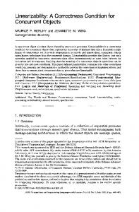
A finite state automaton describing the behavior of a write-snapshot object The non-deterministic automaton of Figure 12 describes in an abbreviated form all the possible behaviors of a write-snapshot object in a system of three processes p, q, and r. To simplify the figure, it is assumed that a process pi proposes i. Each edge correspond to an invocation of write snapshot(), and the list of integers L labeling a transition edge means that the corresponding invocation of write snapshot() is by one of the processes pi such that i ∈ L. The value returned by the object is {L}. Thus, for the linearization of the execution in Figure 3, the path in the automaton goes through states ∅, {1, 2}, {1, 2}, {1, 2, 3}. Any path starting from the initial empty state, and in which a process index appears at most once, defines an execution of the write-snapshot task that does not predict the future. Moreover if, when it executes, a process proceeds from the automaton state s1 to the state s2 , the state s2 defines the tuple of values output by its invocation of write snapshot(). ∅ 1

3

2

2, 3

1, 2 2

1 1, 2, 3

1

2

3

1, 3 3

2

3 1 1, 3

1, 2 1, 2

2, 3

1, 3 3

2 1, 2, 3

2, 3

1 1, 2, 3

Figure 12: A non-deterministic automaton for a write-snapshot object

C C.1

Additional discussion and examples of linearizability limitations Additional examples of tasks with no sequential specification

Several tasks have been identified that are problematic for dealing with them through linearizability. The problem is that they do not have a natural sequential specification. One may consider linearizable implementations of restricted sequential specifications, where if two operations occur concurrently, one is linearized before the other. Thus, in every execution, always there is a first operation. In all cases we discuss below, such an implementation would provably be of a more powerful object. An adopt-commit object [17] is a one-shot shared-memory object useful to implement round-based protocols for set-agreement and consensus. It supports a single operation, adopt commit(). The result of this operation is an output of the form (commit, v) or (adopt, v), where the second component is a value from this set and the 1st component indicates whether the process should decide value v immediately or adopt it as its preferred value in later rounds of the protocol. It has been shown to be equivalent to the conflict detection object [4], which supports a single operation, check(). It returns true or false, and has the following two properties: In any execution that contains a check(v) operation and a check(v ′ ) operation with v 6= v ′ , at least one of these operations returns true. In any execution in which all check operations have the same input value, they all return false. As observed in [4] neither adopt-commit objects nor conflict detectors have sequential specification. A deterministic linearizable implementation of an adopt-commit object gives rise to a deterministic implementation of consensus, which does not exist. Similarly, the first check operation linearized in any execution of a conflict detector must return false and subsequent check operations with different inputs must return true, which can be used to implement test-and-set, for which no deterministic implementation from registers exists. In the safe-consensus problem of [2], the agreement condition of consensus is retained, but the validity condition is weakened as follows: if the first process to invoke it returns before any other process invokes it, then it outputs its input; otherwise the consensus output can be arbitrary, not even the input of any process. There is no sequential specification of this problem, because in any sequential specification, the first process to be linearized would obtain its own proposed value. See Appendix C.3.

iv

Two examples that motivated Neiger are the following [38]. In the immediate snapshot task [7], there is a single operation Immediate snapshot(), such that a snapshot occurs immediately after a read. Such executions play an important role in distributed computability [5, 7, 45]. There is no sequential specification of this task. One may consider linearizable implementations of restricted immediate snapshot behavior, where if two operations occur concurrently, one is linearized before the other, and where the first operation does not return the value by the second. But such an implementation would provably be of a more powerful object (immediate snapshots can be implemented wait-free using only read/write registers), that could simulate test-and-set. The other prominent example exhibited in [38] is the k-set agreement task [11], where processes agree on at most k of their input values. Any linearizable implementation restricts the behavior of the specification, because some process final value would have to be its own input value. This would be an artifact imposed by linearizability. Moreover, there are implementations of set agreement with executions where no process chooses its own initial value.

C.2

Splitting operations to model concurrency

One is tempted to separate an operation into two, an invocation and a response, to specify the effect of concurrent invocations. Consider two operations of an object, op1 () and op2 (), such that each one is invoked with a parameter and can return a value. Suppose we want to specify how the object behaves when both are invoked concurrently. We can separate each one into two operations, inv opi () and resp opi (). When a process wants to invoke opi (x), instead it first invokes inv opi (x), and once the operation terminates, it invokes resp opi (), to get back the output parameter. Then a sequential specification can define what the operation returns when the history is inv op1 (x1 ), inv op2 (x2 ), resp op1 (), resp op2 (). k-Set agreement is easily transformed into an object with a sequential specification, simply by accessing it through two different operations, one that deposits a value into the object and another that returns one of the values in the object. Using a non-deterministic specification that remembers which values the object has received so far, and which ones have so far been returned, one captures the behavior that at most k values are returned, and any of the proposed values can be returned. This trick can be used in any task. Separating an operation into a proposal operation and a returning operation has several problems. First, the program is forced to produce two operations, and wait for two responses. There is a consequent loss of clarity in the code of the program, in addition to a loss in performance, incurred by a two-round trip delay. Also, the intended meaning of linearization points is lost; an operation is now linearized at two linearization points. Furthermore, the resulting object may provably not be the same. A phenomenon that has been observed several times (see, e.g., in [12, 20, 40]) is that the power of the object can be increased, if one is allowed to invoke another object in between the two operations. Consider a test-and-set object that returns either 0 or 1, and the write-snapshot object. It is possible to solve consensus among 2 processes with only one snapshot object and one test-and-set object only if it is allowed to invoke test-and-set in between the write and the snapshot operation. Similarly, consider a safe-consensus object instead of the test-and-set object. If one is allowed to invoke in between the two operations of write-snapshot a safe-consensus object, then one can solve consensus more efficiently [12]. The object corresponding to a task with two operations Let T be a task (I, O, ∆). We will model T as a sequential object OT in which each process can invoke two operations, set and get, in that order. The idea is that set communicates to OT the input value of a process, while get produces an output value to a process. Thus, the unique operation of T is modelled with two operations. The resulting sequential object is non-deterministic. We define OT . The set of invocations and responses are the following: Inv(OT ) = {set(pi , ini ) | (pi , ini ) ∈ I} ∪ {get(pi ) | pi ∈ Π} Res(OT ) = {set(pi , ini ) : OK | (pi , ini ) ∈ I} ∪ {get(pi ) : outi | pi ∈ Π ∧ (pi , outi ) ∈ O} The set of states of OT is Q = {(σ, τ )|σ ∈ I ∧ τ ∈ ∆(σ)}. Intuitively, a set (σ, τ ) represents that the inputs and output OT knows at that state are σ and τ . The initial state of is (∅, ∅). We define δ as follows. Let (σ, τ ) and (σ ′ , τ ′ ) be two states of OT . Then, • If τ = τ ′ , σ 6= σ ′ and σ ′ = {σ ∪ (pi , ini )} ∈ I, then δ((σ, τ ), set(pi , ini )) contains the tuple (set(pi , ini ) : OK, (σ ′ , τ ′ )). • If σ = σ ′ , τ 6= τ ′ and τ ′ = {τ ∪ (pi , outi )} ∈ ∆(σ), then δ((σ, τ ), get(pi )) contains the tuple (get(pi ) : outi , (σ ′ , τ ′ )). Note that for every sequential execution Sb of OT , it holds that τSb ∈ ∆(σSb), where σSb is the input simplex b containing every input vertex in Sb and, similarly, τSb is the output simplex containing every output simplex in S. v

validity(1) → 2

abort() → notAborted

p

validity(2) → 3

abort() → notAborted

q

validity(3) → 2 r p validity(1) resp(2)p abort() notAborted p q validity(2) q resp(3) q abort() notAborted r r validity(3) r resp(2)

Figure 13: An execution of a Validity-Abort object (3)

C.3

Validity and Safe-consensus objects

We first discuss the validity object with abort, and then the safe-consensus object. C.3.1 Validity with abort object An interval-sequential object can be enriched with an abort operation that takes effect only if a given number of processes request an abort concurrently. Here we describe the example of Section 3.3 in more detail, that extends the validity object with an abort operation that should be invoked concurrently by at least k processes. As soon as at least k processes concurrently invoke abort the object will return from then on aborted to every operation. Whenever less than k processes are concurrently invoking abort, the object may return NotAborted to any pending abort. An example appeared in Figure 6, for k = 2. Another example is in Figure 13, where it is shown that even though there are two concurrent abort operations, they do not take effect because they are not observed concurrently by the object. This illustrates why this paper is only about safety properties, the concepts here cannot enforce liveness. There is no way of guaranteeing that the object will abort even in an execution where all processes issue abort at the same time, because the operations may be executed sequentially. The k-validity-abort object is formally specified as an interval-sequential object by an automaton, that can be invoked by either propose(v) or abort, and it responds with either resp(v) or aborted or NotAborted. Each state q is labeled with three values: q.vals is the set of values that have been proposed so far, q.pend is the set of processes with pending invocations, and q.aborts is the set of processes with pending abort. The initial state q0 has q0 .vals = ∅, q0 .pend = ∅ and q0 .aborts = ∅. If in is an invocation to the object different from abort, let val(in) be the proposed value, and if r is a response from the object, let val(r) be the responded value. For a set of invocations I (resp. responses R) vals(I) denotes the proposed values in I (resp. vals(R)). Also, aborts(I) denotes the set of processes issuing an reqAbort in I, and notAborted(R) is the set of processes getting notAborted in R. The transition relation δ(q, I) contains all pairs (R, q ′ ) such that: 1. If r ∈ R then id(r) ∈ q.pend or there is an in ∈ I with id(in) = id(r), 2. If (r = resp(v) ∈ R or notAborted ∈ R) then aborted 6∈ R, 3. If r = resp(v) ∈ R then val(r) = v ∈ q.vals or there is an in ∈ I with val(in) = val(r), 4. If notAborted ∈ R, then 0 < |q.aborts| + |aborts(I)| < k 5. If |q.aborts| + |aborts(I)| ≥ k then aborted ∈ R. 6. q ′ .vals = q.val ∪ vals(I), q ′ .pend = (q.pend ∪ ids(I)) \ ids(R), and q.aborts = (q.aborts ∪ aborts(I)) \ notAborted(R) C.3.2 Safe-consensus Recall that the safe-consensus problem of [2], is similar to consensus. The agreement condition of consensus is retained, but the validity condition is weakened as follows: if the first process to invoke it returns before any other

vi

p q r

scons(x)

p q r

resp(x)

scons(y) scons(z)

p q r

scons(x) scons(y)

scons(x′ ) resp(x)

q3

q1

q0

p q r

resp(x)

q5

resp(z) p q r

p q r

resp(z) scons(y)

scons(x′ ) resp(z)

q4

q2

q6

Figure 14: Part of an interval-sequential automaton of safe-consensus process invokes it, then it outputs its input; otherwise the consensus output can be arbitrary, not even the input of any process. As noticed in Section C.1, there is no sequential specification of this problem. See Figure 14 for part of the automata corresponding to safe-consensus, and examples of interval executions in Figure 15.

Interval execution α1 init term init term p scons(x) resp(x) q scons(y) resp(x) r scons(z) Interval execution α2 init term init term p scons(x) resp(z) q scons(y) resp(z) r scons(z)

init scons(x′ )

term

resp(x)

init scons(x′ )

term

resp(z)

Figure 15: Examples of interval-executions for safe-consensus

D D.1

Tasks Basic definitions

A task is the basic distributed equivalent of a function, defined by a set of inputs to the processes and for each (distributed) input to the processes, a set of legal (distributed) outputs of the processes, e.g., [26]. In an algorithm designed to solve a task, each process starts with a private input value and has to eventually decide irrevocably on an output value. A process pi is initially not aware of the inputs of other processes. Consider an execution where only a subset of k processes participate; the others crash without taking any steps. A set of pairs s = {(id1 , x1 ), . . . , (idk , xk )} is used to denote the input values, or output values, in the execution, where xi denotes the value of the process with identity idi , either an input value, or a output value. A set s as above is called a simplex, and if the values are input values, it is an input simplex, if they are output values, it is an output simplex. The elements of s are called vertices. An input vertex v = (idi , xi ) represents the initial state of process idi , while an output vertex represents its decision. The dimension of a simplex s is |s| − 1, and it is full if it contains n vertices, one for each process. A subset of a simplex is called a face. Since any number of processes may crash, simplexes of all dimensions are of interest, for taking into account executions where only processes in the simplex participate. Therefore, the set of possible input simplexes forms a complex because its sets are closed under containment. Similarly, the set of possible output simplexes also form a complex. More generally, a complex K is a set of vertices V (K), and a family of finite, nonempty subsets of V (K), called simplexes, satisfying: (1) if v ∈ V (K) then {v} is a simplex, and (2) if s is a simplex, so is every nonempty subset of s. The dimension of K is the largest dimension of its simplexes, and K is pure of dimension k if every vii

{p}

σ3

p

{p, q}

∆

p

r {p, q, r}

O

I q

{p, r}

q

σ4 q

r

q

r

{p, q}

{p, r}

p

p

{r}

{q}

q

r

q

{q, r}

q {q, r}

Figure 16: Immediate snapshot task {p}

p {p, r}

{p, q} q

r

Simplex s {p, q, r}

r

q

{p, q}

{p, r}

p

p

p

{r}

{q}

q

r

q

r

{q, r}

{q, r}

Figure 17: Part of the write-snapshot output complex simplex belongs to a k-dimensional simplex. In distributed computing, the simplexes (and complexes) are often chromatic, since each vertex v of a simplex is labeled with a distinct process identity. Definition 2 (Task). A task T for n processes is a triple (I, O, ∆) where I and O are pure chromatic (n − 1)dimensional complexes, and ∆ maps each simplex s from I to a subcomplex ∆(s) of O, satisfying: 1. ∆(s) is pure of dimension s 2. For every t in ∆(s) of dimension s, ID(t) = ID(s) 3. If s, s′ are two simplexes in I with s′ ⊂ s then ∆(s′ ) ⊂ ∆(s). We say that ∆ is a carrier map from the input complex I to the output complex O. A task is a very compact way of specifying a distributed problem, and indeed it is hard to understand what exactly is the problem being specified. Intuitively, ∆ specifies, for every simplex s ∈ I, the valid outputs ∆(s) for the processes in ID(s) assuming they run to completion, and the other processes crash initially, and do not take any steps. The immediate snapshot task is depicted in Figure 16. On the left, the input simplex is depicted and, on the right, the output complex appears. In figure 17 one simplex s is added to the output complex of the immediate snapshot task of Figure 16, where s = {(p, {p, q}), (q, {p, q, r}), (r, {p, q, r})}. This simplex s corresponds to the execution of Figure 4.

D.2

Validity as a task

Recall the validity object is specified as an interval-sequential object in Section 3.3, which is neither linearizable nor set-linearizable. In the usual, informal style of specifying a task, the definition would be very simple: an operation returns a value that has been proposed. A bit more formally, in an execution where a set of processes participate with inputs I (each x ∈ I is proposed by at least one process), each participating process decides a value in I. To illustrate why this informal style can be misleading, consider the execution in Figure 10, where the viii

three processes propose values I = {1, 2, 3}, so according to the informal description it should be ok that they decide values {1, 2, 3}. However, for the detailed interleaving of the figure, it is not possible that p and q would have produced outputs that they have not yet seen. To define validity formally as a task, the following notation will be useful. It defines a complex that represents all possible assignments of (not necessarily distinct) values from a set U to the processes. In particular, all processes can get the same value x, for any x ∈ U . Given any finite set U and any integer n ≥ 1, we denote by complex(U, n) the (n − 1)-dimensional pseudosphere [26] complex induced by U : for each i ∈ [n] and each x ∈ U , there is a vertex labeled (i, x) in the vertex set of complex(U, n). Moreover, u = {(id1 , u1 ), . . . , (idk , uk )} is a simplex of complex(U, n) if and only if u is properly colored with identities, that is idi 6= idj for every 1 ≤ i < j ≤ k. In particular, complex({0, 1}, n) is (topologically equivalent) to the (n − 1)-dimensional sphere. For u ∈ complex(U, n), we denote by val(u) the set formed of all the values in U corresponding to the processes in u. Similarly, for any set of processes P , complex(U, P ) is the |P − 1|-dimensional pseudosphere where each vertex is labeled with a process in P , and gets a value from U . The validity task over a set of values U that can be proposed, is (I, O, ∆), where I = O = complex(U, n). The carrier map ∆ is defined as follows. For each simplex s ∈ I, ∆(s) = complex(U ′ , P ′ ), where P ′ is the set of processes appearing in s and U ′ is their proposed values.

E

Proofs S

Claim 1 The relation −→ is acyclic. S

S

S

Proof For the sake of contradiction, suppose that −→ is not acyclic, namely, there is a cycle C = S1 −→ S2 −→ S

S

S

X . . . −→ Sm−1 −→ Sm , with S1 = Sm . We will show that the existence of C implies that −→ is not acyclic, for some object X, which is a contradiction to our initial assumptions. First note that it cannot be that each Si is a concurrency class of the same object X, because if so then C is

S

S

X X a cycle of −→, which contradicts that −→ is a total order. Thus, in C there are concurrency classes of several objects. op In what follows, by slight abuse of notation, we will write S ′ −→ S ′′ if S ′ and S ′′ are related in Sb because of S the second case in the definition of −→. op op op Note that in C there is no sequence S1 −→ S2 −→ S3 because in Sb whenever T ′ −→ T ′′ , we have that T ′ is

op

S

X a responding class and T ′′ is an invoking class, by definition. Thus, in C there must be a sequence S1 −→ S2 −→ op SX SY SX SX b we have S2 −→ . . . −→ St −→ St+1 −→ St+2 . Observe that in S, St since −→ is transitive, hence the sequence

op

S

op

S

X Y can be shortened: S1 −→ S2 −→ St −→ St+1 −→ St+2 . Note that S1 and St are responding classes while S2 and St+1 are invoking classes. op op Now, since S1 −→ S2 , there are operations a, b ∈ OP such that a −→ b, a ∈ S1 and b ∈ S2 . Similarly, for op op St −→ St+1 , there are c, d ∈ OP such that c −→ d, c ∈ St and d ∈ St+1 . This implies that term(a) < init(b) op op b we have S1 −→ and term(c) < init(d). Observe that if we show a −→ d then, by definition of S, St+1 , if S1 and

op

S

S

X Y St+1 otherwise. Hence, the sequence S1 −→ S2 −→ St+1 are concurrent classes of distinct objects, and S1 −→

op

op

S

S

S

S

Y Y Y Y St −→ St+1 −→ St+2 can be shortened to S1 −→ St+1 −→ St+2 or S1 −→ St+1 −→ St+2 . Repeating this

S

S

X X enough times, in the end we get that there are concurrency classes Si , Sj in C such that Si −→ Sj −→ Si , which

S

X is a contradiction since −→ is acyclic, by hypothesis. op To complete the proof of the claim, we need to show that a −→ d, i.e., term(a) < init(d). We have four cases: op 1. if b = c, then term(a) < init(b) < term(b) = term(c) < init(d), hence a −→ d.

op

op

2. If b −→ c, then term(a) < init(b) < term(b) < init(c) < term(c) < init(d), hence a −→ d. op SX SX b X = (SX , −→) 3. If c −→ b, then we have that St −→ S2 , because each S| respects the real time order in S

S

X X comp(E|X ), by hypothesis. But we also have that S2 −→ St , which contradicts that −→ is a total order. Thus this case cannot happen.

op

op

4. If b and c are concurrent, i.e., b 9 c and c 9 b, then note that if init(d) ≤ term(a), then term(c) < op init(d) ≤ term(a) < init(b), which implies that c −→ b and hence b and c are not concurrent, fro which follows that term(a) < init(d). ix

✷Claim 1 Theorem 3 Let E be an interval-linearizable execution in which there is a pending invocation inv(op) of a total operation. Then, there is a response res(op) such that E · res(op) is interval-linearizable. Proof Since E is interval-linearizable, there is an interval-linearization Sb ∈ ISS(X) of it. If inv(op) appears b we are done, because Sb contains only completed operations and actually it is an interval-linearization of in S, b E · res(op), where res(op) is the response to inv(op) in S. Otherwise, since the operation is total, there is a responding concurrency class S ′ such that Sb · {inv(op)} · S ′ ∈ ISS(X), which is an interval-linearization of E · res(op), where res(op) is the response in S ′ matching inv(op). ✷T heorem 3 function sequences (E) is i ← 1; e ← first event in E; F ← empty execution σ0 , τ0 ← ∅; A ← σ0 ; B ← τ0 ; while F 6= E do if (e is an invocation) then if (τi \ τi−1 = ∅) then σi ← σi ∪ {e} else σi+1 ← σi ∪ {e}; τi+1 ← τi ; A ← A · σi ; B ← B · τ i ; i ← i + 1 end if else τi ← τi ∪ {e} end if; F ← F · e; e ← next event to e in E end while; A ← A · σi ; B ← B · τi ; return (A, B).

Figure 18: Producing a sequence of faces of the invocation simplex σ and response simplex τ of an execution E. For the rest of the section we will often use the following notation. Let E be an execution. Then, σE and τE denote the sets containing all invocations and responses of E, respectively. Claim 2. For every execution E, the function sequences() in Figure 18 produces sequences A = σ0 , . . . , σk and B = τ0 , . . . , τm such that 1. k = m. 2. σ0 = ∅ ⊂ σ1 ⊂ . . . ⊂ σm−1 ⊂ σm = σE and τ0 = ∅ ⊂ τ1 ⊂ . . . ⊂ τm−1 ⊆ τm = τE . 3. If E has no pending invocations, then τm−1 ⊂ τm , otherwise τm−1 = τm 4. If E satisfies a task with carrier map ∆, then, that for each i, τi ∈ ∆(σi ). 5. For every response e and invocation e′ in E such that e precedes e′ and they do not match each other, we have i < j, where i is the smallest integer such that e ∈ τi and j is the smallest integer such that e′ ∈ σj . 6. For every response e of E in τi \ τi−1 , σi contains all invocations preceding e in E. Proof Items (1), (2) and (6) follow directly from the code. For item (3), note that if E has no pending invocations, it necessarily ends with a response, which is added to τm , and thus τm−1 ⊂ τm . For item (4), consider a pair σi and τi , and let E ′ be the shortest prefix of E that contains each response in τi . Note that the simplex containing all invocations in E ′ is σi . Since, by hypothesis, E satisfy T , it follows that τi ∈ ∆(σi ). For item (5), consider such events e and e′ . Since e precedes e′ , the procedures analyzes first e, from which follows that it is necessarily true that i ≤ j, so we just need to prove that i 6= j. Suppose, by contradiction, that i = j. Consider the beginning of the while loop when e′ is analyzed. Note that e′ ∈ / σi at that moment. Also, note that e ∈ τi \ τi−1 because i is the smallest integer such that e ∈ τi and its was analyzed before e′ . Thus, when the procedure process e′ , puts it in σi+1 , which is a contradiction, because in the final sequence of simplexes e′ ∈ / σi . ✷Claim 2 Theorem 4 For every task T , there is an interval-sequential object OT such that any execution E satisfies T if and only if it is interval-linearizable with respect to OT . x

Proof The structure of the proof is the following. (1) First, we define OT using T , (2) then, we show that every execution that satisfies T , is interval-linearizable with respect to OT , and (3) finally, we prove that every execution that is interval-linearizable with respect to OT , satisfies T . Defining OT : Let T = hI, O, ∆i. To define OT , we first define its sets with invocations, response and states: Inv = {(id, x) : {(id, x)} ∈ I }, Res = {(id, y) : {(id, y)} ∈ O } and Q = {(σ, τ ) : σ ∈ I ∧ τ ∈ O}. The interval-sequential object OT has one initial state: (∅, ∅). Then OT will have only one operation and so the name of it does not appear in the invocation and responses. The transition function δ is defined as follows. Consider an input simplex σ of T and let E be an execution that satisfies T with σE = σ and τE ∈ ∆(σE ). Consider the sequences σ0 = ∅ ⊂ σ1 ⊂ . . . ⊂ σm = σE and τ0 = ∅ ⊂ τ1 ⊂ . . . ⊂ τm = τE that Sequences in Figure 18 produces on E. Then, for every i = 1, . . . , m, δ((σi−1 , τi−1 ), σi \ σi−1 ) contains ((σi , τi ), τi \ τi−1 ). In other words, we use the sequences of faces to define an interval-sequential execution (informally, a grid) that will be accepted by OT : the execution has 2m concurrency classes, and for each i = 1, . . . , m, the invocation (pj , −) (of process pj ) belongs to the 2i − 1-th concurrency class if (pj , −) ∈ σi \ σi−1 , and the response to the invocation of appears in the 2i-th concurrency class if (pj , −) ∈ τi \ τi−1 . We repeat the previos construction for every such σ and E. If E satisfies T , it is interval-linearizable: Consider an execution E that satisfies T . We prove that E is interval-linearizable with respect to OT . Since E satisfies T , we have that τE ∈ ∆(σE ). By definition, ∆(σ) is dim(σ)-dimensional pure, then there is a dim(σ)-dimensional γ ∈ ∆(σ) such that τE is a face of γ. Let E be an extension of E in which the responses in γ \τE are added in some order. Thus, there are no pending operation in E. Consider the sequences of simplexes produced by Sequences in Figure 18 on E. As we did when defined OT , b We have the following: (1) Sb is an interval-sequential the two sequence define an interval-sequential execution S. b execution of OT , by construction, (2) for every p, S|p = E|p , by construction, and (3) Claim 2.5 implies that Sb op op b = (OP, −→) respect the real-time order of invocations and responses in E: if op1 −→ op2 in the partial order OP associated to E, then, by the claim, the response of op1 appears for the first time the sequence in τi and the invocation of op2 appears for the first in the sequence in σj , with i < j, and hence, by construction, op1 precedes b We conclude that Sb is an interval-linearization of E. op2 in S. If E is interval-linearizable, it satisfies T : Consider an execution E that is interval-linearizable with respect to OT . We will show that E satisfies T . There is an interval-sequential execution Sb that is a linearization of E, since E is interval-linearizable. Consider any prefix E ′ of E and let Sb′ be the shortest prefix of Sb such that (1) it is an interval-sequential execution and (2) every completed invocation in E ′ is completed in Sb′ (note that there might be pending invocations in E ′ that does not appear in Sb′ ). By construction, Sb′ defines two sequences of simplexes σ0 = ∅ ⊂ σ1 ⊂ . . . ⊂ σm and τ0 = ∅ ⊂ τ1 ⊂ . . . ⊂ τm with τi ∈ ∆(σi ), for every i = 1, . . . , m. Observe that σE ′ = σm and τE ′ ⊆ τm , and thus τE ′ ∈ ∆(σE ′ ) because τm ∈ ∆(σm ). What we have proved holds for every prefix E ′ of E, then we conclude that E satisfies T . ✷T heorem 4 Lemma 1 There is a sequential one-shot object O such that there is no task TO , satisfying that an execution E is linearizable with respect to O if and only if E satisfies TO (for every E). Proof Consider a restricted queue O for three processes, p, q and r, in which, in every execution, p and q invoke enq(1) and enq(2), respectively, and r invokes deq(). If the queue is empty, r’s dequeue operation gets ⊥. Suppose, for the sake of contradiction, that there is a corresponding task TO = (I, O, ∆), as required by the lemma. The input complex I consists of one vertex for each possible operation by a process, namely, the set of vertices is {(p, enq(1)), (q, enq(2)), (r, deq())}, and I consists of all subsets of this set. Similarly, the output complex O contains one vertex for every possible response to a process, so it consists of the set of vertices {(p, ok), (q, ok), (r, 1), (r, 2), (r, ⊥)}. It should contain a simplex σx = {(p, ok), (q, ok), (r, x)} for each value of x ∈ {1, 2, ⊥}, because there are executions where p, q, r get such values, respectively. See Figure 19. Now, consider the three sequential executions of the figure, α1 , α2 and α⊥ . In α1 the process execute their operations in the order p, q, r, while in α2 the order is q, p, r. In α1 the response to r is 1, and if α2 it is 2. Given that these executions are linearizable for O, they should be valid for TO . This means that every prefix of α1 should be valid: {(p, ok)} = ∆((p, enq(1)) {(p, ok), (q, ok)} ∈ ∆({(p, enq(1), (q, enq(2)}) σ1 = {(p, ok), (q, ok), (r, 1)} ∈ ∆({(p, enq(1), (q, enq(2), (r, deq())}) = ∆(σ) xi

σ1 ok 1

enq(1)

r

enq(2)

ok

q

O

I

σ

q

r

∆

p

σ⊥

p

⊥

r

deq()

σ2 r 2

→ ok

→ ok

p

p

→ ok

→ ok

α2 q

α1 q →1

→2

r

r → ok

p → ok

α3 q →2

r

Figure 19: Counterexample for a simple queue object Similarly from α2 we get that σ2 = {(p, ok), (q, ok), (r, 2)} ∈ ∆(σ) But now consider α3 , with the same sequential order p, q, r of operations, but now r gets back value 2. This execution is not linearizable for O, but is accepted by TO because each of the prefixes of α3 is valid. More precisely, the set of inputs and the set of outputs of α2 are identical to the sets of inputs and set of outputs of α3 . ✷Lemma 1 Theorem 5 For every one-shot interval-sequential object O with a single total operation, there is a refined task TO such that any execution E is interval-linearizable with respect to O if and only if E satisfies TO . Proof The structure of the proof is the following. (1) First, we define TO using O, (2) then, we show that every execution that is interval-linearizable with respect to O, satisfies TO , and (3) finally, we prove that every execution that satisfies TO , is interval-linearizable with respect to O. Defining TO : We define the refined task TO = (I, O, ∆). First, since O has only one operation, we assume that its invocation and responses have the form inv(pj , xj ) and res(pj , yj ). Let Inv and Res be the sets with the invocations and responses of O. Each subset σ of Inv containing invocations with different processes, is a simplex of I. It is not hard to see that I is a chromatic pure (n − 1)-dimensional complex. O is defined similarly: each subset τ of Res × 2Inv containing responses in the first entry with distinct processes, is a simplex of O. We often use the following construction in the rest of the proof. Let E be an execution. Recall that σE and τE are the simplexes (sets) containing all invocations and responses in E. Let τ0 = ∅ ⊂ τ1 ⊂ . . . ⊂ τm = τE and σ0 = ∅ ⊂ σ1 ⊂ . . . ⊂ σm = σE be the sequences of simplexes produced by Sequences in Figure 18 on E. These sequences define an output simplex {(res, σi ) : res ∈ τi \ τi−1 } of TO , which will be denoted γE . We define ∆ as follows. Consider an input simplex σ ∈ I. Suppose that E is an execution such that (1) σE = σ (2) it has no pending invocations and (3) it is interval-linearizable with respect to O. Note that dim(σ) = dim(τE ) and ID(σ) = ID(τE ). Consider the simplex γE induced by E, as defined above. Note that dim(σ) = dim(γE ) and ID(σ) = ID(γE ). Then, ∆(σ) contains γE and all its faces. We define ∆ by repeating this for each such σ and E. Before proving that T is a task, we observe the following. Every dim(σ)-simplex γE ∈ ∆(σ) is induced by an execution E that is interval-linearizable. Let Sb be an interval-linearization of E. Then, for any execution F such that γF = γE (namely, Sequences produce the same sequences on E and on F ), Sb is an interval-linearization b p , and (3) Sb of F : (1) by definition, Sb is an interval-sequential execution of O, (2) for every process p, F |p = S| xii

respects the real-time order of invocations and response in F because it respects that order in E and, as already said, they have the same sequence of simplexes and, by Claim 2.5, these sequences reflect the real-time order of invocations and responses. We argue that T is a refined task. Clearly, for each σ ∈ I, ∆(σ) is a pure and chromatic complex of dimension dim(σ), and for each dim(σ)-dimensional τ ∈ ∆(σ), ID(τ ) = ID(σ). Consider now a proper face σ ′ of σ. By definition, each dim(σ ′ )-dimensional simplex γE ′ ∈ ∆(σ ′ ) corresponds to an execution E ′ whose set of invocations is σ ′ , has no pending invocations and is interval-linearizable with respect to O. Let Sb′ be an intervallinearization of E ′ and let s′ be the state O reaches after running Sb′ . Since the operation of O is total, from the state s′ , the invocations in σ \ σ ′ can be invoked one by one until O reaches a state s in which all invocations in σ have a matching response. Let Sb be the corresponding interval-sequential execution and let E be an extension of E ′ in which (1) every invocation in σ \ σ ′ has the response in Sb and (2) all invocations first are appended in some order and then all responses are appended in some (not necessarily the same) order. Note that Sb′ is a prefix of Sb and actually Sb is an interval-linearization of E. Then, ∆(σ) contain the dim(σ)-simplex γE induced by E. Observe that γE ′ ⊂ γE , hence, ∆(σ ′ ) ⊂ ∆(σ). Finally, for every dim(σ)-simplex γE ∈ ∆(σ), for every vertex (idi , yi , σi ) of γE , we have that σi ⊆ σ because γE is defined through an interval-linearizable execution E. Therefore, we conclude that TO is a task. If E is interval-linearizable, it satisfies TO : Consider an execution E that is interval-linearizable with respect to O. We prove that E satisfies TO . Since E is interval-linearizable, there is an interval-linearization Sb of it. Let E ′ be any prefix of E and let Sb′ be the shortest prefix of Sb such that (1) it is an interval-sequential execution and (2) every completed invocation in E ′ is completed in Sb′ (note that there might be pending invocations in E ′ that does not appear in Sb′ ). Note that Sb′ is an interval-linearization of E ′ . Since interval-linearizability is non-blocking, Theorem 3, there is an interval-linearization Sb′′ of E ′ in which every invocation in E ′ has a response. Let E ′′ be an extension of E ′ that contains every response in Sb′′ (all missing responses are appended at the end in some order). Note that σE ′ = σE ′′ and τE ′ ⊆ τE ′′ . Consider the output simplexes γE ′ and γE ′′ induced by E ′ and E ′ . Observe that γE ′ ⊆ γE ′′ (because E ′ differs from E ′′ in some responses at the end). By definition of TO , γE ′′ ∈ ∆(σE ′ ), and hence γE ′ ∈ ∆(σE ′ ). This holds for every prefix E ′ of E, and thus E satisfies TO . If E satisfies TO , it is interval-linearizable: Consider an execution E that satisfies TO . We prove that E is interval-linearizable with respect to O. Let γE be the output simplex induced by E. Since E satisfies TO , γE ∈ ∆(σE ). Since ∆(σE ) is a pure dim(σE )-dimensional complex, there is a dim(σ)-simplex γE ∈ ∆(σE ) such that γE ⊆ γE . Observe that σE = σE while τE ⊆ τE . Therefore, E is an extension of E in which the responses in τE \ τE are appended in some order at the end of E. Now, by construction, γE ∈ ∆(σE ) because there is an interval-sequential execution Sb of O that is an interval-linearization of E. We have that Sb is an intervallinearization of E as well because, as already mentioned, E is an extension of E in which the responses in τE \ τE are appended in some order at the end. ✷Lemma 5

xiii