Linearizability and Schedulability

www.hurray.isep.ipp.pt

Technical Report Linearizability and Schedulability

Björn Andersson HURRAY-TR-071004 Version: 0 Date: 10-22-2007

Technical Report HURRAY-TR-071004

Linearizability and Schedulability

Linearizability and Schedulability Björn Andersson IPP-HURRAY! Polytechnic Institute of Porto (ISEP-IPP) Rua Dr. António Bernardino de Almeida, 431 4200-072 Porto Portugal Tel.: +351.22.8340509, Fax: +351.22.8340509 E-mail: http://www.hurray.isep.ipp.pt

Abstract Consider the problem of scheduling a set of tasks on a single processor such that deadlines are met. Assume that tasks may share data and that linearizability, the most common correctness condition for data sharing,must be satisfied.We find that linearizability can severely penalize schedulability. We identify, however, two special cases where linearizability causes no or not too large penalty on schedulability.

© IPP Hurray! Research Group www.hurray.isep.ipp.pt

1

Linearizability and Schedulability Bj¨orn Andersson IPP-HURRAY! Research Group, Polytechnic Institute of Porto (ISEP-IPP), Rua Dr. Ant´onio Bernardino de Almeida 431, 4200-072 Porto, Portugal [email protected]

Abstract Consider the problem of scheduling a set of tasks on a single processor such that deadlines are met. Assume that tasks may share data and that linearizability, the most common correctness condition for data sharing, must be satisfied. We find that linearizability can severely penalize schedulability. We identify, however, two special cases where linearizability causes no or not too large penalty on schedulability.

1. Introduction Consider the problem of preemptive scheduling of n sporadically arriving tasks on a single processor where tasks may share data. A task τi is given a unique index in the range 1..n. A task τi generates a (potentially infinite) sequence of jobs. The time when these jobs arrive cannot be controlled by the scheduling algorithm and the time of a job arrival is unknown to the scheduling algorithm before the job arrives. It is assumed that the time between two consecutive jobs from the same task τi is at least Ti . It is assumed that there is a single shared data object in the system. A job may invoke an operation on that data object and the data object will generate a response back to the job (for example, if the shared data object is a linked list then invoking an operation may be requesting to insert an element in the list and the response may be a boolean specifying whether the list was empty before insertion). We assume that linearizability [1], the most common correctness criteria for data sharing, must be satisfied. In order to define linearizability we need two other definitions. A history is a sequence of invocations and responses made on an object by a set of tasks. A sequential history is a history in which all invocations have immediate responses. Linearizability is satisfied if every history that

can occur to the shared data object is linearizable. A history is linearizable if all these three conditions are true: C1. invocations and responses of the history can be reordered to yield a sequential history; C2. that sequential history is correct according to the sequential definition of the object; C3. if a response preceded an invocation in the original history, it must still precede it in the sequential reordering. The execution of a job is as follows. A job needs to perform Ci time units in order to finish execution and among that, Ciop of the execution is due to executing an operation on the shared data object. Clearly it holds that Ciop ≤ CP i . The processor utilization is defined as n i U processor = i=1 C Ti . The utilization of the shared data P Ciop n object is U op = i=1 Ti . The utilization is defined as U = max(U processor , U op )1 . It is required that the job finishes the execution at most Ti time units after its arrival. In order to satisfy the deadlines and linearizability, a real-time scheduling algorithm S and a data sharing protocol DP is used. We assume that 0 ≤ Ci ≤ Ti . Also, recall that we have already mentioned that Ciop ≤ Ci . It is assumed that Ci , Ciop and Ti are real numbers. It is common to characterize the performance of scheduling algorithms using the utilization bound. The utilization bound U B(S, DP ) of the composition of the scheduling algorithm S and the data sharing protocol DP is the maximum number such that if all tasks are scheduled by S and operations on the shared data object are controlled by DP and if U ≤ U B(S, DP ) then all tasks meet their deadlines 1 The careful reader can see that since C op ≤ C it follows that i i U op ≤ U processor and hence the max function in the expression of U is redundant. We define utilization in this way though because (i) it can be easily extended to multiprocessor systems and (ii) it can be used to show which resource (processor or the shared data object) is the ”‘bottleneck”’.

and all operations on the shared data object satisfies linearizability. It is interesting to ask whether it is possible to design S and D such that U B(S, DP ) > 0. In this paper, we show that for every S and D, it holds that U B(S, DP )=0. This low performance is caused by the fact that C3 must be satisfied. As a consequence, we address two special cases which are less penalized by C3 and for those special cases we find that U B(S, DP ) = 1 and U B(S, DP ) = 0.5 respectively can be achieved. The remainder of this paper is organized as follows. Section 2 discusses how linearizability limits schedulability. Section 3 discusses a special case where only read operations and write operations are performed on the shared data object. Section 4 discusses the special case where the time required for each operation is the same. Finally, Section 5 gives conclusions.

Using actual numbers gives us that it must be possible to perform 1/L + 1 units of execution during a time interval of duration 1. This is clearly impossible and hence it follows that it is impossible to schedule this task set such that all deadlines are met and linearizability is satisfied. We can do this reasoning for every choice of L. Letting L → ∞ yields a task set with U → 0 and still a deadline is missed.

3. Only Read/Write operations The low utilization bound caused by linearizability follows from the fact that we made no assumption on the operations offered by the shared data object. We will now consider a special type of shared data object with only two possible operations: read the entire data from the shared object or write data to the entire shared object. An efficient shared data object with these operations has been proposed [3]. The main idea is that a vector stores pointers to different versions of the object. When a task invokes a request to write to the object, it finds empty space and writes the new object there. And then, it writes a pointer to this new version in the vector (using the atomic Compareand-Swap instruction). A task invoking a read operation will obtain a pointer to the last pointer that was inserted in the vector. Observe that writes are performed on new buffers and hence a read operation will never ”see” a partially updated object. Also observe that the response of a write operation does not depend on any previous reads and hence it is easy to find a sequential order and consequentially this object is linearizable. The scheme also recycles memory buffers in the vector in order to be able to operate with a finite amount of memory. This scheme (which we call TZ-Buffer) can be used together with EDF and it has U B(EDF, TZ − Buffer) = 1; assuming that the overhead within the data-object (finding an empty buffer, etc.) is zero.

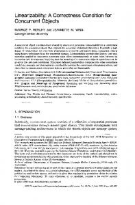
2. Linearizability It is easy to see that for every scheduling algorithm and for every data-sharing protocol, the composition of these causes the utilization bound to be zero because linearizability must be satisfied. Example 1 shows this. Example 1. Figure 1 illustrates the task set in the example. Consider two tasks characterized as T1 =1,C1 = C1op =1/L, T2 =L and C2 = C2op =1. We choose L >2. Let us consider an arbitrary job released by τ2 . Let A2 denote the arrival time of that job. We know that in order to meet deadlines, this job must finish C2 time units within [A2 , A2 + T2 ). We also know that in order to satisfy linearizability, the response given by the shared data object is equal to some sequential order (according to C1). Let SEQ denote this sequential order. Then it holds that this sequential order SEQ must be < . . ., OP 1′ , OP 2, OP 1′′ , . . . > where OP 1′ and OP 1′′ denote two different operations by τ1 and OP2 denotes an operation by τ2 . If we ignore the deadline constraints then it is possible to schedule tasks (and hence the operations) such that such an order exist and hence linearizability would be satisfied. Let us now reason about linearizability and satisfying deadlines. Consider the sequential order SEQ. Since we do not assume any specific shared data object; the response given by OP 1′′ may depend on OP 2 and the response by OP 2 may depend on OP 1′ . This follows from C2. Because of this dependency, it follows that the correct response can only be achieved through scheduling the jobs such that this sequential history is achieved. That is, it must be that a job from τ1 is executed and then a job from τ2 is executed nonpreemptively and this job from τ2 must finish its execution before the next job of τ1 starts executing. Hence it must be possible to perform C1 +C2 units of execution a time interval of duration T1 .

4. Equal execution time for operations Example 1 in Section 2 showed that the utilization bound can be 0 because linearizability must be satisfied. In the example, the execution times of the tasks were very different. This is reasonable in many real-world applications. For example one task may perform sampling and it inserts the data in a buffer and it has a very small execution time. Another task reads data from the buffer, performs processing and outputs the result on a display and it has a very large execution time. Despite the fact that execution times of tasks may be very different; it is often the case that the operations on shared data objects are small and the execution times are approximately the same. Consider for example a FIFO queue; the 2

Figure 1. An example of a task set with utilization arbitrary close to zero and it misses a deadline because linearizability must be satisfied. An arrow pointing upwards indicates the arrival time of a job.

time required to perform insert and remove is approximately the same. Also, consider a hierarchical data structure (as a tree). Searching, adding and deleting typically have time complexities O(log k), where k is the number of elements, and hence the difference in execution times cannot be too high assuming that there is an upper bound on the number of elements. It has also been observed that in practice many operations on shared data objects have a short execution time [4, 5]. For these reasons, we will now consider the case where ∀i, j : Ciop = Cjop . We will consider Earliest-DeadlineFirst (EDF) scheduling [2]. At time t, it assigns priorities to jobs that have arrived at time t but have not yet finished execution. Let A(Ji ) denote the arrival time of a job Ji . Then the priority of job Ji is higher than the priority of job Jj if A(Ji ) + Ti < A(Jj ) + Tj . We will consider the nonpreemptive critical-section (NPCS) protocol. It means that all operations on the shared data object are protected by a critical section and when a task executes in the critical section, it executes non-preemptively; when the task leaves the critical section, the task can be preempted again. The performance of EDF with the NPCS protocol is provided by Theorem 1.

Let us consider the earliest time when a deadline was missed. M denotes one of those jobs. Ai denotes the arrival time of M . τi denotes the task that released M . Let us consider two cases: 1. Ci /Ti > 0.5 This contradicts Equation 2. 2. Ci /Ti ≤ 0.5 Let us reason about this case. t1 denotes the deadline of M and t0 denotes the latest time such that t0 < t1 and the processor is busy during [t0 , t1 ) and the processor is idle just before t0 . For convenience we let L denote t1 − t0 . We know that [t0 , t1 ) must be non-empty since Ci > 0 and Ti > 0. Let us define two classes of tasks: (3)

τ classB,i = {τj : (Tj ≥ Ti ) ∧ (j 6= i)}

(4)

end

Let us consider a task τj in τ classA,i . If τj arrived after time t1 − Tj then its deadline is later than t1 and hence it will have a lower priority than M . Also observe that such a job from task τj arrives after Ai because Tj < Ti . Hence this job cannot cause any delay to the job M . Consequently, we delete this job released by τj and then M still misses its deadline. For this reason we obtain that the amount of work performed by task τj in τ classA,i during [t0 , t1 ) is at most:

TheoremP 1. Consider a task set such that ∀i, j : Ciop = n op Cj and j=1 Cj /Tj ≤ 1/2 and this task set is scheduled by EDF and the NPCS protocol. We claim that this task set meets all deadlines. Proof. The proof is by contradiction. Suppose that the theorem was incorrect. Then there must exist a task set such that: ∀i, j : Ciop = Cjop

τ classA,i = {τj : Tj < Ti }

(1) max(⌊

and n X

Cj /Tj ≤ 1/2

(2)

L − Tj ⌋ + 1, 0) · Cj Tj

(5)

Let us now consider a task τj in τ classB,i . If none of these jobs executed just after time Ai then we obtain that the amount of work performed by task τj in τ classB,i during [t0 , t1 ) is at most:

j=1

and the task set is scheduled by EDF and the NPCS protocol and at least one deadline was missed. 3

Simplifying Equation 13 yields: max(⌊

L − Tj ⌋ + 1, 0) · Cj Tj

n X L L ⌊ ⌋ · Ci > T 2 i j=1

(6)

Let us now consider a task τj in τ classB,i . If one of these jobs executed just after time Ai then let τj denote this task. Observe that this task may release a job with a lower priority than M but it will still execute in [t0 , t1 ). The amount of execution it will perform is Cjop . With reasoning similar to Equation 5-6 we obtain that the amount of work performed by this task τj in τ classB,i during [t0 , t1 ) is at most:

Cjop + max(⌊

L − Tj ⌋ + 1, 0) · Cj Tj

Dividing by L and relaxing yields: n X Ci j=1

L − Ti ⌋ + 1, 0) · Ci Ti

n X

max(⌊

j=1

L − Ti ⌋ + 1, 0) · Ci Ti

We have seen that satisfying linearizability causes the utilization bound to drop to 0. We also saw two special cases where the utilization is greater than zero. It deserves to find out which data objects can be shared while attaining a non-zero utilization bound. For those data objects where the utilization bound necessarily is zero it deserves to find (i) limitations on the task sets for which the utilization bound is non-zero and (ii) whether alternative correctness criteria can be used.

(8)

Acknowledgements (9) This work was partially funded by the Portuguese Science and Technology Foundation (Fundac¸a˜ o para Ciˆencia e Tecnologia - FCT) and the ARTIST2 Network of Excellence on Embedded Systems Design.

References

(10)

[1] M. P. Herlihy and J. M. Wing. Linearizability: a correctness condition for concurrent objects. ACM Transactions on Programming Languages and Systems (TOPLAS), 12(3):463– 492, May 1990. [2] C. L. Liu and J. W. Layland. Scheduling algorithms for multiprogramming in a hard real-time environment. Journal of the Association for the Computing Machinery, 20:46–61, 1973. [3] P. Tsigas and Y. Zhang. Non-blocking data sharing in multiprocessor real-time systems. In Proc. of Real-Time Computing Systems and Applications, pages 247–254, Hong Kong, China, Dec. 13–15, 1999. [4] P. Tsigas and Y. Zhang. Evaluating the performance of nonblocking synchronization on shared-memory multiprocessors. In Proc. of ACM SIGMETRICS Performance Evaluation, pages 320–321, Massachusetts, USA, June 17–20, 2001. [5] P. Tsigas and Y. Zhang. Integrating non-blocking synchronisation in parallel applications: performance advantages and methodologies. In Proc. of the 3rd international workshop on Software and performance, pages 55–67, Rome, Italy, July 24–26, 2002.

Simplifying yields that the amount of work performed by all tasks during [t0 , t1 ) is at most: n

(11)

Since a deadline is missed it must be that: Ti X L ⌊ ⌋ · Ci > L + 2 Ti j=1 n

(12)

Since τi was the task that missed a deadline, it follows that Ti ≤ L. Using it on Equation 12 and rewriting yields: L X L ⌊ ⌋ · Ci > L + 2 j=1 Ti

(15)

5. Conclusions

n

Ti X L ⌊ ⌋ · Ci + 2 Ti j=1

1 2

(7)

We know that Cjop = Ciop and Ciop ≤ Ci and that Ci ≤ Ti /2. Using this on Equation 9 yields that the amount of work performed by all tasks during [t0 , t1 ) is at most: L − Ti Ti X max(⌊ ⌋ + 1, 0) · Ci + 2 Ti j=1

>

We can see that regardless of the case we obtain a contradiction. And hence the theorem is true.

Taking Equation 5-8 together and simplifying yields that the amount of work performed by all tasks during [t0 , t1 ) is at most: Cjop +

Ti

But this contradicts Equation 2.

It is also clear that for task τi we have that the amount of work performed by task τi during [t0 , t1 ) is at most: max(⌊

(14)

n

(13)

4