We introduce Scene Structural Matrix (SSM), a novel image content descriptor and its application to invariant image retrieval. The SSM captures the overall ...
Spectral and Spatial Invariant Image Retrieval using Scene Structural Matrix G. Qiu and S. Sudirman School of Computer Science The University of Nottingham {qiu, sxs} @ cs.nott.ac.uk Abstract We introduce Scene Structural Matrix (SSM), a novel image content descriptor and its application to invariant image retrieval. The SSM captures the overall structural characteristics of the scene by indexing the geometric features of the image. We employ a binary image tree (bintree) to partition the image and from which we derive multiscale geometric structural descriptors of the image. We have applied the SSM to contentbased image retrieval from image databases. Experimental results show that SSM is particularly effective in retrieving images with strong structural features, such as landscape photographs. We will show that SSM is robust against spatial and spectral distortions thus making it superior to current state of the art techniques such as colour correlogram in certain applications. We will also show that images retrieved by the SSM are more relevant than those returned by colour correlogram and colour histogram.
1. Introduction Managing large image databases is an important area of research. The important research issues in this area including image indexing and retrieval. In particular, contentbased indexing and retrieval methods [1] have attracted extensive research interests in recent years. Traditional methods use global statistics of local image features, e.g., colour histogram [2], colour correlogram [3] and their variance as image indices. These methods have been shown to be very successful in retrieving images with similar local feature distributions. However, since these measures do not take into accounts the locations of the local features, the retrieved results often do not make a lot of sense. For example, using a landscape image with blue sky on top and green countryside at the bottom as query example and trying the retrieve images with similar structures, i.e., blue sky on top and green countryside at the bottom, methods based on global statistics of local features often give very unsatisfactory results. Another scenario is one in which two or more images of the same scene photographed under different imaging conditions, e.g., images of a countryside taken at dusk or dawn under a clear or a cloudy sky. Using one of these images as a query example often fails to retrieve other images of the same scene taken under different time or conditions. In yet another situation maybe one in which a same scene imaged by different, uncalibrated devices. Using one image taken by one device may fail to find the same scene taken by other devices. In this paper, we introduce a new method for content-based image indexing and retrieval. We first present a method which uses a binary image tree [8] to partition an image recursively into hierarchical sub-images. Then we introduce the Scene Structural Matrix (SSM), a 2-dimensional table to summarize the geometric structures of the partitioned image. We use the SSM as image indices for content-based image retrieval.
373
Experiments have been performed on an image database consisting of over 7000 highresolution photographic colour images. It is shown that the SSM is particularly effective in retrieving images with strong structural features such as landscape images. It is also shown that the SSM is more robust to spatial and spectral distortions than traditional color histogram and state of the art color correlogram methods and therefore is advantageous in applications such as retrieving images of the same scene imaged at different time and under different imaging conditions. The organization of the paper is as follows. Section 2 describes the scene structural matrix. Section 3 presents the application of SSM to content based image retrieval. Section 4 presents experimental results and section 5 concludes the paper.
2. Deriving Scene Structural Content Descriptors In this section, we present the concept of the method used to construct the SSM. The main idea is to collect the geometry features of an image and tabulate them in a compact manner to be used as image content index for the purpose of achieving content-based image retrieval. In what follows we will first present a simple constraint adaptive image segmentation method and then describe the process of constructing the SSM from the segmented image.
2.1 Binary Tree Image Segmentation To construct the SSM, we first segment the image using a simple, easy to implement, binary image tree (bintree) adaptive image segmentation method [8], which can be regarded as a much simplified version of binary space partitioning tree image segmentation method [4-6]. An image (assumed rectangular in shape) is first cut into two equal sized subimages by either a vertical or a horizontal straight line. Each of the resulting two subimages is again cut into two equal sized sub-images by either a vertical or a horizontal straight line. The process is repeated for each of the subsequent subimages until a stopping criterion (e.g., when the pixel value variation in the sub-image falls below a preset value) is reached. Figure. 1 illustrates such a scheme. 1
1
1
f
e
C1
A1
0.5
a
A2
B2
B1
0.5
D1 0.5
c
b
d
F2
G1
G2
E1 E2
D2
C2
F1
g 0
0
0.5
1
0
0
0.25
0.5
1
0
0
0.250.375 0.5
0.75
1
Figure 1. The bintree adaptive image segmentation scheme. The original image is partitioned by the vertical line a into two equal sized halves (left); Lines b and c partition the resulting two halves (middle); and the resulting four subimages are partitioned by the lines d, e, f and g (right). The capital letters denote the characteristics of the corresponding region. They might represent the region average color, the distribution of color or even textures.
Whether a subimage (including the original) is cut by a horizontal or a vertical line depends on the structure of the subimage (hence the segmentation is adaptive), and there are many criterion can be used. A simple method is the least-square fit. First, it uses a vertical line to cut the sub-image into two equal sized halves and approximate the pixels in each half by the average colours of their respective half and calculate the square error of such approximation. Another square error value is calculated for the horizontal cut
374
image segmentation. The cut, which gives the smaller approximation error, is chosen. . Let S(i, j), i = 0, 1, ... M-1, j = 0, 1, ..., N-1, be an M x N subimage to be partitioned, and 2 MCl = M ×N
N −1 M −1 2
∑ ∑ S (i, j ) i =0 j =0
MCr =
2 M ×N
M −1 N −1
2 M ×N
M −1 N −1
∑ ∑ S (i, j ) i =0
j=
N 2
(1)
M
MCt =
2 M ×N
−1 2 N −1
∑∑ S (i, j ) i =0 j =0
MCb =
∑∑ S (i, j )
i=
M j=0 2
N −1 M −1 N −1 1 M −1 2 2 2 MSEV = ∑ ∑ (S (i, j ) − MCl ) + ∑ ∑ (S (i, j ) − MC r ) M × N i =0 j =0 N i =0 j= 2 M 2 −1N −1 M −1 N −1 1 2 2 MSE h = ∑ ∑ (S (i, j ) − MCt ) + ∑ ∑ (S (i , j ) − MCb ) M × N i =0 j =0 M j =0 i= 2
(2)
If MSEv > MSEh, then cut the subimage vertically, otherwise cut it horizontally Another method is to cut the subimages based on the predominant edge orientations. In this method, the horizontal and vertical gradients are first calculated and the subimage is cut based on the magnitudes of the directional gradients. If the vertical gradient dominates, then the sub-image is cut horizontally, otherwise vertically. Many well-know edge detection operators [7] can be used to calculate the directional gradients. Let Gh(i, j) and Gv(i,j), i = 0, 1, ... M-1, j = 0, 1, ..., N-1, be the horizontal and vertical gradients respectively, of an M x N subimage to be partitioned. We calculate Gh =
1 M ×N
M −1 N −1
∑∑ G (i, j ) i =0 j =0
h
Gv =
1 M ×N
M −1 N −1
∑∑ G (i, j ) i =0 j =0
v
(3)
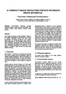
If Gh > Gv, the subimage will be cut vertically otherwise horizontally. Figure 2 shows an example of the segmentation.
2.2 Construction of Scene Structural Matrix Based on the bintree segmented image, we construct a table termed scene structural matrix. The rationale for building the SSM is that because the reconstruction are perceptually similar to the original, then the features from the reconstruction can be used to recognise the original. The fact that we recursively cut the image with only horizontal and vertical lines means that there are some very simple geometry structures can be extracted. When a line partitions a sub-image, it intersects with the two borders of the sub-image which are perpendicular to it forming a T shape structure at different resolutions (refer to Figure 1, the dash and solid lines). It is based on this T shape structure we build our scene structural matrix. The SSM is a two dimensional array indexing the T shape structures of the bintree segmented image. There are only two types of T shape structures and their conjugates. Therefore only the � � DQG the structures need to be indexed since ( and ) and ( and ) will always appear in pairs. It is clear, at different level and depending on how a subimage is cut, the two arms of the T-shape features will have different length. The SSMs capture this fact by indexing the T-shape features of various sizes. There are two SSMs, SSM and SSM
375
indexing the two unique T-shape features. Each cell in the matrix corresponds to the Tshape with a certain arm lengths. The values of the cells in SSM are the accumulated average color difference across the horizontal arm, and the values of the cells in SSM are the accumulated average color differences across the vertical arm. The formal description of the SSM is as follows: Let hi = H/2i, vj = V/2j, where i, j = 0, 1, 2, … are two integers, H is the horizontal dimension of the image and V is vertical dimension of the image.
Figure 2, From top to bottom clockwise: Original landscape image, 1st, 3rd, 5th, 7th, 9th, 10th, 11th, and 12th level partition. Each subimage is painted by its average colour.
Let ha and va be the lengths of horizontal arm and vertical arm of the T shape features. We have SSM (i , j) �660 (ha = hi and va = vj) = ACC | Ctop - Cbottom | (4) SSM (i , j) �660 (ha = hi and va = vj) = ACC | Cleft - Cright | where ACC denotes accumulation, and Ctop is the average colour of the top half and Cbottom is the average colour of the bottom half of the partition. Similarly, Cleft is the average colour of the left half and Cright is the average colour of the right half of the partition. As an example, Figure 3 shows the SSMs of the scene partitions of Figure 1. SSM
SSM
0
0
0
|A1-A2|
|B1-B2|
|E1-E2|
|C1-C2|
0
x
0
|F1-F2| + |G1-G2|
x
|D1-D2|
x
x
0
x
x
Figure 3 The Scene Structural Matrices (SSM) of the segmentation of Figure 1. The capital letters denote the average colour vectors of their corresponding sub-images
376
3. Content-based Image Indexing and Retrieval using SSM We can use the SSMs as image indices for content-based indexing and retrieval in image database application. The SSMs for each image in the database are constructed and image retrieval can be based on comparing these SSMs with that of the query image. It is worth noting that only a few (5 to 8) levels of partition suffice, hence the size of SSM is very small. Let SSMq(i, j) and SSMd(i, j) be the SSMs of the query image and the database image respectively. The similarity of the two images can be calculated by D (q, d) = min { D1(q, d), D2(q, d) }
(5)
D1(q, d) = ΣiΣj ( W(i,j)(|SSM q(i, j)- SSM d(i, j)| + |SSM q(i,j)- SSM d(i,j)|))
(6)
D2(q, d) = ΣiΣj ( W(i,j)(|SSM q(i,j)- SSM d(i,j)| + |SSM q(i,j)- SSM d(i,j)| ))
(7)
The min {} operator guarantees a zero difference between identical images rotated by ±90°. The matrix W(i,j) allows us to use different weights to the contribution of coarse and detail features of the image. Intuitively we would like global features to be more dominant than detail features. A typical weight matrix is
0 1 2
0 1 ½ 1/3
1 ½ 1/3 x
2 1/3 x x
Based on image similarity measures calculated according to (5), images that have smaller distances are considered more similar to the query and are returned to the user.
4. Experimental Results We have implemented the SSM method for image indexing and retrieval using an image database of 7400 high-resolution colour photographic images, a subset of the commercially available Corel Photo collection widely used by other research groups. From the database, we randomly chose 50 landscape images (for display convenience, 49 of which are shown in Figure 4). In the experiment, each of these images was subjected to various spatial and spectral processing before being used as query image. The aim was to use the distorted (processed) image as query and retrieve the original image from the database. The processing performed include spectral (colour) modification, spatial resolution scaling, and spatial filtering. As a comparison, we have also implemented colour histogram (CH) [2] (4096-bin) and colour correlogram (CC) [3] (4 distances, 64 colors) methods. For the results presented, the SSMs were built based on 7 level bintree partitions. The cumulative recall rate, i.e., the number of retrieved original images above a certain rank, of various processed images as queries and using different query methods are shown in Tables 1 - 3. These tables should be interpreted as follows: For example, in table 1, when the query images were subjected to colour distortion, SSM retrieved 2 (out of 50) target images in the 1st rank, CC retrieved none in the 1st rank, CH also retrieved none in the 1st rank etc. Similarly, in table 2, when the query images were subjected to spatial scaling, SSM retrieved 37 (out of 50) target images in the 1st rank, CC retrieved none in the 1st rank; CH retrieved all targets in the 1st rank etc. Table 3 should be interpreted similarly.
377
Figure 4. Examples of query images. The images have been re-scaled to square for display purpose. The original dimensions of the images were not all square.
Ranks Methods SSM CC CH
1 2 0 0