Spectral calibration of hyperspectral imagery using

Spectral calibration of hyperspectral imagery using atmospheric absorption features Luis Guanter, Rudolf Richter, and José Moreno

One of the initial steps in the preprocessing of remote sensing data is the atmospheric correction of the at-sensor radiance images, i.e., radiances recorded at the sensor aperture. Apart from the accuracy in the estimation of the concentrations of the main atmospheric species, the retrieved surface reflectance is also influenced by the spectral calibration of the sensor, especially in those wavelengths mostly affected by gaseous absorptions. In particular, errors in the surface reflectance appear when a systematic shift in the nominal channel positions occurs. A method to assess the spectral calibration of hyperspectral imaging spectrometers from the acquired imagery is presented in this paper. The fundamental basis of the method is the calculation of the value of the spectral shift that minimizes the error in the estimates of surface reflectance. This is performed by an optimization procedure that minimizes the deviation between a surface reflectance spectrum and a smoothed one resulting from the application of a low-pass filter. A sensitivity analysis was performed using synthetic data generated with the MODTRAN4 radiative transfer code for several values of the spectral shift and the water vapor column content. The error detected in the retrieval is less than ⫾0.2 nm for spectral shifts smaller than 2 nm, and less than ⫾1.0 nm for extreme spectral shifts of 5 nm. A low sensitivity to uncertainties in the estimation of water vapor content was found, which reinforces the robustness of the algorithm. The method was successfully applied to data acquired by different hyperspectral sensors. © 2006 Optical Society of America OCIS codes: 280.0280, 110.0110, 120.4640, 120.6200.

1. Introduction

Imaging spectrometers are being increasingly used in the remote sensing of the Earth system processes. The large amount of narrow observation channels makes hyperspectral sensors a useful tool for exploitation of the information contained in discrete absorption features of both atmosphere and surface constituents. The depth, shape, and spectral location of these features are key variables in the characterization of the corresponding natural species in either solid, liquid, or gaseous states. Therefore an accurate spectral and radiometric calibration is needed to guarantee the reliability of the extracted information.

L. Guanter ([email protected]) and J. Moreno are with the Department of Thermodynamics, University of Valencia, Dr. Moliner 50, 46100 Burjassot, Valencia, Spain. R. Richter is with the Remote Sensing Data Center, German Aerospace Center (DLR), D-82234 Wessling, Germany. Received 20 October 2004; revised 23 May 2005; accepted 24 May 2005. 0003-6935/06/102360-11$15.00/0 © 2006 Optical Society of America 2360

APPLIED OPTICS 兾 Vol. 45, No. 10 兾 1 April 2006

The spectral and radiometric calibration is usually performed in a laboratory (preflight calibration). However, the instrument performance might change after launch into space or after installation in an aircraft, because of processes such as outgassing, aging of optical or electronic components, and misalignment due to mechanical vibrations. In particular, spectral shifts and channel broadenings are very likely to appear in detector arrays mounted in the focal plane of imaging sensors. Thus postlaunch calibration campaigns are often conducted to check the accuracy or stability of the laboratory calibration.1–5 For broadband sensors with channels in the atmospheric window regions, such as Landsat–TM or Systeme Probatoire pour l’Observation de la Terre (SPOT), small changes in the spectral properties would be difficult to detect. Investigations are restricted to an update of the absolute radiometric calibration. A different situation exists for hyperspectral instruments6 –9 with typical narrow bandwidths of 5–15 nm. These instruments cover large contiguous parts of the solar spectrum, and the recorded radiance signature contains the absorption features of atmospheric gases (e.g., 760 nm oxygen absorption,

940 nm water vapor absorption). Small shifts of the center wavelength of those channels located in atmospheric absorption regions will lead to errors in the retrieved surface reflectance, usually perceptible images, i.e., radiances recorded at the sensor aperture, by the appearance of spikes and dips in the spectra. An accurate analysis of the influence of spectral shifts in the registered at-sensor radiance is made in Ref. 10. Simulated data with a systematic spectral shift of 1 nm for channels of 10 nm full width at half-maximum (FWHM) showed associated errors in the measured radiance of up to ⫾25% in strong water vapor absorption bands. Similar results are presented in Ref. 11. Recent work by Gao et al.12 presented a method to detect spectral shifts in spectrometers, using a spectrum-matching technique applied to at-sensor radiances, with atmospheric absorption features as a reference. This contribution presents a method to evaluate spectral shifts in hyperspectral sensors. Our approach is closely coupled to the atmospheric correction procedure. The resulting surface reflectance spectra are not only free from the atmospheric distortion, but also free from the errors caused by systematic spectral shifts. In this way, spectral shifts are calculated on the basis of surface reflectance instead of on a radiance basis. This simplifies the modeling problem and speeds up the process considerably, without a perceptible loss of accuracy. The main assumption is that the spectral shift may change in the across-track direction of the acquired image line, but that the nominal bandwidths remain constant. Nonlinear effects in the spectral calibration usually occur in pushbroom sensors, built with CCD area arrays, owing to the “smile” effect.13 A CCD matrix measures a spatial image line in one of its dimensions and in the other dimension it measures the spectrally dispersed radiance for each pixel along the image line. This causes nonlinear features in the spectral response of the detector arrays placed in the focal plane. Detectors in the extreme of the array may have different behaviors from those located in the center leading to a change in the value of the spectral shift along the across-track direction. On the other hand, spectral shifts are expected to be constant for whiskbroom sensors, built with linear detector arrays, in which the image scan line is acquired by the rotation and oscillation of a scan mirror. However, nonlinear behavior might also appear due to manufacturing or alignment errors. The basis of the method is a 1D optimization procedure that minimizes the errors in the estimates of surface reflectance as a function of the spectral shift. These errors manifest themselves as spikes and dips in the spectra appearing around gaseous absorptions after atmospheric correction of the at-sensor radiances. Each step of the iterative optimization procedure varies the value of the shift with respect to the nominal channel wavelength centers. When the highresolution atmospheric parameters used in the atmospheric correction are convolved with the updated

band configuration, the errors in the surface reflectance disappear to a large extent. Therefore the output of the procedure is not only the characterization of the spectral performance of the instrument, but also the surface reflectance free from the distortion caused by a potentially inaccurate spectral calibration. A detailed description of the method, a sensitivity analysis, and the results obtained from the application to a set of different hyperspectral sensors are presented in this paper. 2. Methodology

In the case of perfectly calibrated hyperspectral sensors, the only cause of error spikes in atmospherically corrected spectra would be a possible misevaluation of the gaseous concentrations in the atmospheric correction, commonly H2O, but also O2 and CO2. However, if an accurate water vapor retrieval is performed on a pixel-by-pixel basis, the spikes are most likely caused by a systematic shift in the position of the channel center wavelengths. The usual procedure in atmospheric correction is to use radiative transfer codes to calculate the atmospheric radiance and transmittance functions needed for the evaluation of the atmospheric contribution to the at-sensor radiances. Those codes produce high spectral resolution outputs that have to be convolved with the spectral response function of each channel. Then the resulting resampled functions are used in the retrieval of the surface reflectance from the atsensor data. The proposed idea is to calculate the spectral shift that would produce the smoothest surface reflectance spectra when applied to the convolution with the channel response functions in the generation of the atmospheric parameters. The determination of the shift is made by a 1D optimization procedure that minimizes the difference between a spiky shifted spectrum and the corresponding smoothed reference spectrum, the spectral shift being the variable of the inversion. The first step is to calculate an average spectrum from all the pixels in the same along-track line, to have a representative sampling of the sensor performance in the across-track direction. Images with a large spectral contrast in either the along-track or the across-track directions (e.g., scenes with mixed land and water targets) must not be used, as the average spectra would not be statistically representative. In this way, a vector of spectra representing the average spectral signature in the across-track direction is obtained. The procedure described hereinafter is applied to all of those averaged spectra. It starts with the atmospheric correction of the measured at-sensor radiances. The usual Lambertian assumption14 is made to formulate the spectral at-sensor radiance L,

L共␭兲 ⫽ L0共␭兲 ⫹

Eg共␭兲 ␳ ␭ ␶ ␭ ⫹ ␶dif共␭兲兴, ␲ 共兲关 dir共兲

(1)

where ␳ is the surface reflectance, L0 is the path 1 April 2006 兾 Vol. 45, No. 10 兾 APPLIED OPTICS

2361

radiance for a black ground, Eg is the global flux (i.e., direct plus diffuse) on the ground, and ␶dir and ␶dif are the direct and diffuse transmittances (ground to sensor), respectively. The required reflectance ␳ can be easily obtained by the inversion of Eq. (1). The water vapor column content in the scene can be estimated by using one of the available water vapor retrieval algorithms15,16 adapted to the particular band configuration of the sensor. In our implementation, the water vapor column is calculated from the image using the atmospheric precorrected differential absorption (APDA) algorithm15 on a pixel-bypixel basis. As will be shown later, a precise value of the spectral shift can also be calculated with a rough water vapor column estimate 共⫾0.5 g cm⫺2兲. This means that a high accuracy in the water vapor column content is not a strict requirement in the determination of the shift, as the computation is based on the reference spectrum smoothness in relative terms. Therefore major error spikes caused by a spectral miscalibration will be eliminated, but some residual spikes or dips might be retained in case of an inaccurate water vapor column estimate. This is an important issue, since the water vapor retrievals might be affected by the underlying spectral shift for extreme values. Thus the estimation of the water vapor from external sources, such as ground measurements when available, would be recommended when a strong miscalibration was expected. Aerosols are not as significant as water vapor in the appearance of punctual errors because their contribution does not cause signal modifications at specific wavelengths, but they affect a spectrum in a continuous way over a wide spectral region. Thus climatology values of aerosol total loading and aerosol type can be assumed in those cases where the interest is only in the spectral shift calculation and not in the surface reflectance retrieval itself. Once atmospheric parameters are specified, we use the MODTRAN4 radiative transfer code,17 setting the spectral resolution to 1 cm⫺1, to calculate L0, Eg, ␶dir, and ␶dif in Eq. (1) for all the average along-track pixels in the across-track direction. This code has been chosen here because of its high spectral resolution and its rigorous formulation of the coupling between atmospheric absorption and scattering. The hyperspectral output from MODTRAN4 is convolved to the nominal band configuration. The resulting surface reflectance spectrum is likely to present artifacts in the vicinity of atmospheric absorption bands, partially or totally because of a systematic spectral shift in the focal plane array. To have a reference for the calculation of the spectral shift ␦, this first spectrum is smoothed using a low-pass filter, ␳i smooth ⫽

1 i⫹m 兺 ␳j共␦兲, N j⫽i⫺m

m⫽

N⫺1 . 2

(2)

where ␳i smooth is the surface reflectance in the channel number i after the application of the filter, and N is an odd integer number giving the number of neighbors to 2362


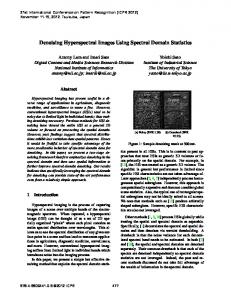
Fig. 1. Surface reflectance spectrum derived from a synthetic at-sensor radiance spectrum (where a ⫹2.0 nm spectral shift was added to a typical hyperspectral sensor band setting) before and after applying the smoothing given in Eq. (2). The reflectance spectrum obtained using the shifted wavelengths is offset by ⫹20% for clarity. The thin curve corresponds to the atmospheric transmittance spectrum for the same configuration.

be averaged. We chose N ⫽ 5 because it is enough for a proper smoothness of the spectrum without losing the original shape. The spectrum ␳i smooth is highly independent of ␦ because of the application of the filter. Figure 1 shows the results of the atmospheric correction of a MODTRAN4 synthetic at-sensor radiance spectrum, compared with an atmospheric transmittance spectrum. The band configuration corresponds to standard hyperspectral specifications, with bandwidths of approximately 10 nm. A systematic spectral shift of 2.0 nm was added in the generation of the at-sensor radiance. The resulting surface reflectance spectrum obtained using the shifted channels (offset curve) presents errors in the surroundings of gaseous absorption bands. The strong water vapor absorption channels centered at 1400 and 1900 nm were removed from the plot because the signal at those wavelengths is often very low and noisy. The theoretical (shift-free) spectrum is also plotted, jointly to the smooth spectrum after applying Eq. (2) showing a very good agreement. The smoothed spectrum is taken as a reference in the calculation of the spectral shift that is retrieved by means of an optimization procedure: the merit function ␹2 to be minimized is Nc

␹2共␦兲 ⫽ 兺关␳i surf共␦兲 ⫺ ␳i smooth兴2,

(3)

i⫽1

where ␳i surf共␦兲 is the surface reflectance in channel i calculated assuming a spectral shift of ␦, and Nc is the number of channels in the spectrometer, skipping those affected by the strongest absorptions, i.e., those located in the spectral ranges 1300–1500 nm and 1800–2000 nm. The inversion is performed in an iterative way, in which each iteration varies the value of ␦. The shifted channel filter function is used in the resampling of the MODTRAN4 output. The initial at-sensor radiance spectrum extracted from the image is used to calculate a

Fig. 3. Estimation of the relative error in the surface reflectance caused by different values of the spectral shift (expressed in nanometers) for the particular inputs used in the generation of the synthetic data set given in Section 3.

3. Sensitivity Analysis A.

Fig. 2. Flow chart of the main steps of the spectral shift method, to be applied to all the pixels in the average cross-track direction array. The shaded boxes represent the inputs provided by the user.

different ␳i surf共␦兲 during each iteration, following the procedure previously described: The hyperspectral output from MODTRAN4 is convolved with the channel response functions to derive the atmospheric variables appearing in Eq. (1) that are used to transform from at-sensor radiance to surface reflectance. Response functions Si共␭; ␦兲 are simulated using Gaussian functions as it is usually done in the case of imaging spectrometers,

冋冉

Si共␭; ␦兲 ⫽ exp ⫺

共␭ ⫺ ␭c共i兲 ⫺ ␦兲 C ␴i

冊册

Synthetic Data Set

A detailed sensitivity analysis18 of the algorithm performance was performed to assess the method’s robustness against extreme values of the spectral shift and uncertainties in the water vapor column content. A total of 100 radiance spectra were generated according to Eq. (1) with the HyMap (Ref. 6) 2003 band configuration. We selected the HyMap sensor for the sensitivity analysis because it covers a wide wavelength range (⬃400 –2500 nm) separated in four different spectrometers, and their spectral specifications are representative of most spectrometers currently used in remote sensing. In the 2003 configuration, the four HyMap spectrometers cover the regions 438 – 874 nm, 878 –1340 nm, 1404 –1807 nm, and 1951–2483 nm, with an average bandwidth of approximately 15 nm. Most of the results obtained for this configuration can be extrapolated to other sensors with a similar or smaller wavelength sampling. Constant spectral shifts in the band centers ranging from ⫺5 to ⫹5 nm in 0.1 nm steps were added in the four spectrometers. The atmospheric quantities (path ra-

2

,

(4)

where ␭c共i兲 is the nominal center wavelength of channel i, C is a constant that has to be initially adjusted according to normalization criteria, and ␴i is the nominal FWHM of channel i. Note the ␦ dependence in the Si共␭; ␦兲 calculation. The final output of the inversion is the value of ␦ that provides the smoothest surface reflectance spectrum. A flow chart describing the whole process is displayed in Fig. 2.

Fig. 4. Values of ε(␦) in Eq. (5) for the synthetic data set as a function of the simulated shift. 1 April 2006 兾 Vol. 45, No. 10 兾 APPLIED OPTICS

2363

Fig. 5. Comparison between input and retrieved value of the spectral shift for the four HyMap spectrometers for a perfect guess in the water vapor column content. The right axes show the absolute difference between simulated and retrieved values. All the values are given in nanometers.

diance, transmittance, global flux) were calculated with the MODTRAN4 code. The input parameters were a flight altitude of 4 km, ground elevation at 0.7 km above sea level (ASL), a solar zenith angle of 25°, a mid-latitude summer atmosphere with a 23 km visibility for aerosols, and 1.6 g cm⫺2 of water vapor column content. A mixed spectrum, built with a linear combination of one bare soil and one pure vegetation spectra, was selected as the input surface reflectance spectrum. The relative error in surface reflectance caused by the simulated shifts of HyMap channels in such a configuration is displayed in Fig. 3. Large errors of up to 55% are reached in the strongest water vapor absorption bands centered at approximately 1400

and 1900 nm. This fact justifies that they are not taken into account in the computation of the merit function in Eq. (3). Important errors up to 20% are also found in weaker absorption bands across the 400–2500 nm wavelength range, mostly due to water vapor, but also to oxygen 共around 760 nm兲 and carbon dioxide 共around 2000 nm兲. B.

Validation of the Smoothing Approach

To quantify the validity of using the smooth spectrum as a reference for the calculation of the shift, an error function ␧共␦兲 evaluating the deviation between the smoothed spectrum and the real spectrum has been defined as

Table 1. Values of RMSD for Five Different Water Vapor Contents in Each HyMap Spectrometers ⫺2

WV (g cm 1.0 1.4 1.6 1.8 2.0

2364

)

RMSD sp.1 (nm)

RMSD sp.2 (nm)

RMSD sp.3 (nm)

RMSD sp.4 (nm)

0.380 0.391 0.361 0.360 0.355

0.473 0.323 0.309 0.277 0.279

2.851 0.651 0.665 0.868 1.498

0.158 0.252 0.348 0.376 0.544


Fig. 6. Comparison between input and retrieved value of the spectral shift for the four HyMap spectrometers, for a 0.6 g cm⫺2 error in the water vapor column content. The right axes show the absolute difference between simulated and retrieved values. All values are given in nanometers.

N 冑兺i⫽1 关␳itheor ⫺ ␳i smooth共␦兲兴2 , N ␳itheor 兺i⫽1

C.

c

␧共␦兲 ⫽

c

(5)

where ␳i theor is the theoretical spectrum used as the input in the simulations. The values of ␧共␦兲 calculated for the simulated data set are plotted in Fig. 4. It can be stated that the smoothing approach works better for small values of the shift, while the deviation grows with the absolute value of the shift almost linearly. This is because the largest error spikes and dips cannot be removed by a simple low-pass filter but need more complex strategies. An example of those small residuals is displayed in Fig. 1, near the regions of 920, 1000, and 1100 nm. Most of the spectral range covered by the spectrometers is used in the computation of the merit function to be minimized. Bands affected by the residuals of the spikes are only a small fraction of all bands. The method works in relative terms, searching for the shift that achieves a maximum removal of errors in the reflectance spectrum. Therefore round shapes in the smoothed spectrum do not introduce a large error in the retrievals, because these are a valid reference for the comparison with a sharp peak.

Sensitivity to Spectral Shift

The method was then applied to the synthetic data set, assuming a perfect water vapor retrieval (water vapor content was set to the input value of 1.6 g cm⫺2), to focus only on the method’s capabilities for spectral shift discrimination. Results are plotted in Fig. 5. A comparison between the input theoretical spectral shift and the retrieved values is shown for each one of the four HyMap spectrometers. The worst performance of the method occurs for the largest values of ␦. For ␦ near the extreme value of 5.0 nm, the deviation between the theoretical and the retrieved shifts may be approximately ⫾1.0 nm, and some saturation trends appear in the retrievals. This is an a priori expected behavior, as such large spectral shifts lead to the loss of an important part of band information content. ␦ values higher than 3 nm are unusual in the real case, according to the current technical specifications5 in sensor design. For ␦ values up to 2 nm, the spectral shift is generally retrieved to within an uncertainty range of ⫾0.2 nm. The retrievals for the third spectrometer are less accurate than for the others. The reason is that there are no small or medium absorption features in the 1 April 2006 兾 Vol. 45, No. 10 兾 APPLIED OPTICS

2365

Fig. 7. Spectral shift in the cross-track direction for the four HyMap spectrometers in the 2004 spectral configuration.

wavelength range covered by this spectrometer. Only the two strong absorption features centered at 1400 and 1900 nm are present, which are not taken into account in the shift evaluation due to the difficulties in measurements and radiative transfer calculations in those bands. This means that there are no reference absorption bands to be used for the discrimination of spectral shift. However, since the absence of those reference absorptions also results in a smaller dependence on the spectral shift in the measurements made by this spectrometer, a poorer evaluation of the spectral shift can be tolerated. It will only have a minor effect on the retrieved surface reflectance in this spectral region. D. Sensitivity to Water Vapor

To check the dependence of the shift retrievals on water vapor uncertainties, a similar analysis was performed for several water vapor contents, with a simulated error of up to 0.6 g cm⫺2 (1.0, 1.4, 1.6, 1.8, and 2.0 g cm⫺2 water vapor column contents were used). The root mean square deviation (RMSD) was used for a quick comparison of the results for different water vapor amounts and HyMap spectrometers, accounting for the deviation between theoretical and retrieved values. The values of the RMSD for five different water vapor contents are displayed in Table 1. It confirms that the spectral shift retrievals are not dependent on the estimated water vapor content in the general case, because the method works to minimize the errors in the surface reflectance caused by a spectral shift, disregarding the water vapor miscalculation. Very small values of the RMSD are obtained for spectrometers 1, 2, and 4, independently of the input water vapor. Again, the situation is different for spectrometer 3, as the results are highly dependent on the water vapor due to the lack of reference absorption channels. This translates into large values of the RMSD for this spectrometer when the water vapor column content deviates significantly (1.0 and 2366


2.0 g cm⫺2 cases) from the 1.6 g cm⫺2 value used in the simulation, a factor of 2– 4 larger than the values obtained when water vapor values are closer to the input value (cases 1.4 and 1.8 g cm⫺2). Figure 6 shows a comparison between simulated and retrieved ␦ values for a water vapor in retrievals of 1.0 g cm⫺2. It can be stated that the performance of the method is quite similar to the ideal case of 1.6 g cm⫺2, except for the third spectrometer, as we already discussed, where the deviation is very important. Because of such an underestimation of water vapor content, the resulting surface reflectance spectrum will present large miscorrected absorption features, especially in the wavelengths more affected by water vapor. However, even inside these bands, the smoothness in the shift-corrected spectrum is important compared with the spectrum affected by the systematic shift. Apart from the third spectrometer case, the method works consistently in the retrieval of the spectral shift, even under conditions with a large water vapor uncertainty, which proves the reliability and robustness of the approach. 4. Results A.

Available Data Set

The methodology described has been applied to remotely sensed data acquired by a number of hyperspectral instruments with different specifications. First, the spectral calibration of the HyMap sensor6 has been assessed. HyMap provides hyperspectral information in 126 bands, between 0.445 and 2.480 ␮m in its 2004 configuration. HyMap consists of four different spectrometers working in the whisk-broom mode, with a field of view (FOV) of 60° (512 pixels). Roughly speaking, the first spectrometer covers the wavelength range 0.45–0.90 ␮m, with bandwidths of 15–16 nm and an average sampling interval of 15 nm; the second spectrometer operates in the 0.89–1.35 ␮m range with the same bandwidths and sampling intervals as the first one; the third spectrometer covers the 1.4–1.8 ␮m range with bandwidths of 15–16 nm and an average sampling interval of 13 nm; the fourth spectrometer measures the 1.95–2.48 ␮m range, with bandwidths of 18–20 nm and a sampling interval of 17 nm. The same technique was applied to different scenes of the airborne visible infrared imaging spectrometer (AVIRIS),7 operated by the NASA Jet Propulsion Laboratory (JPL). It delivers calibrated images of the upwelling spectral radiance in 224 contiguous spectral channels, allowing it to cover the entire range between 380 and 2500 nm, separated in four different whisk-broom spectrometers (0.37– 0.68, 0.66 – 0.92, 0.93–1.26, and 1.25–2.51 ␮m, respectively). It is claimed to be calibrated to within 1 nm. The method was also applied to data acquired by the reflective optics system imaging spectrometer8 (ROSIS) in its 2003 configuration. The sensor works following a push-broom principle, making use of a CCD array for imaging simultaneously 115 spectral

Fig. 8. Surface reflectance spectra in HyMap spectrometer 2 for a concrete field and a bare soil target from the Wessling scene for a concrete field (top curves) and a bare soil target (bottom curves). The dashed line and the shaded area represent the average over the ASD ground radiometer measurements and its standard deviation.

bands of 512 picture elements perpendicular to the flight direction. The spectral range is 430–860 nm, with 7.5 nm as a nominal bandwidth. Finally, to assess the validity of the method in the preprocessing of not only airborne sensors, but also spaceborne sensors, it was applied to data from the compact high-resolution imaging spectrometer (CHRIS), onboard the European Space Agency (ESA) Project for Onboard Autonomy (PROBA)9 CHRIS operates in a push-broom mode over the visible and near-infrared bands from 400 to 1050 nm, and can measure in 62 spectral bands with a minimum spectral sampling interval between 1.25 nm (at 400 nm) and 11 nm 共at 1000 nm兲. B.

lated from the image data itself employing the APDA algorithm15 on a per-pixel basis. The method starts with the original laboratory-based calibration file and iterates with the algorithm explained in Section 2 to obtain the final channel center wavelengths. The spectral calibration of the four HyMap spectrometers is depicted in Fig. 7. It was calculated from a scene near Wessling, Germany 共latitude ⫽ 48.02° north, longitude ⫽ 11.28° east), acquired 7 June 2004. The solar zenith angle was 32.1°, the solar azimuth was 226.8° heading north, the flight altitude was 2.59 km ASL, and the ground elevation was 0.6 km ASL. The main point to be noted is that the spectral shift is nearly constant in the across-track direction, as it is expected for whiskbroom instruments. The different performance of the method for the four spectrometers is also noticeable, and the conclusions extracted from the sensitivity analysis are confirmed to a large extent: the largest fluctuations in the shift value across the samples are found in the third spectrometer. This is explained by the lack of absorption bands to be used as a reference in the computation of the shift. The retrieved curves are smoother for the other spectrometers, especially in the first and the second spectrometers. Figure 8 shows a comparison between surface reflectance derived before and after updating the spectral calibration, from the same Wessling scene. For demonstration and visual clarity, results are only shown in a smaller spectral region covered by HyMap’s spectrometer 2. The thin curve corresponds to HyMap-derived spectra based on the laboratory wavelength file as supplied by Integrated Spectronics, and the thick curve presents the results obtained after spectral recalibration. The spectral shifts of the center wavelengths are ⫺1.3 nm with respect to the original laboratory calibration. The reflectance errors near 0.94 and 1.13 ␮m (atmospheric water vapor absorption regions) are successfully removed after reca-

HyMap Imagery

Within the framework of a European airborne campaign in 2004, the HyMap spectrometer collected imagery of approximately 100 flight lines in different countries. The campaign was conducted by Deutsche Forschungsanstalt fur Luft und Raumfahrt (DLR), which also processed the level 2 (orthorectified, atmospherically corrected) data. For a check of the spectral calibration, a certain number of scenes, separated by a few days, was chosen. Then, from each of these scenes, four to eight homogeneous targets were manually selected. Boxes of typically 5 ⫻ 5 pixels 共up to 9 ⫻ 9 pixels兲 were placed in these fields (asphalt, concrete, soil, and dry vegetation) and the corresponding box-averaged surface reflectance and digital number (DN) (scaled at-sensor radiance) spectra were saved as files. The surface reflectance spectrum of each target was calculated with the ATCOR code19,20 based on lookup tables derived from the MODTRAN4 code according to the estimated or measured visibility. The water vapor column was calcu-

Fig. 9. Wavelength shift in spectrometer 2 of HyMap as a function of the day of the 2004 campaign. 1 April 2006 兾 Vol. 45, No. 10 兾 APPLIED OPTICS

2367

Fig. 10. AVIRIS spectra before and after recalibration for vegetation and bare soil targets.

libration. The dashed curve and the shaded area in the plot for the concrete field represent the average and standard deviation of approximately 100 ground measurements conducted with an ASD Fieldspec radiometer (Analytical Spectral Devices, Inc.). The reflectance spectrum of this field shows stable behavior over the years. Therefore a comparison of these ground measurements (conducted on May 11, 2004) with the image-derived spectrum (June 7, 2004) is adequate and supports the results of the proposed spectral calibration method. An interesting issue is the temporal stability of a sensor’s spectral calibration. As an example, Fig. 9 shows the spectral shift of HyMap’s spectrometer 2 as a function of the day of the European campaign 2004, which started on 18 May 2004. The spectral shift is nearly constant, i.e., ⫺1.2 nm 共⫾0.2 nm standard deviation) over a time period of approximately 3 months. In that period the instrument was installed and deinstalled in two different DLR aircraft with a short break of 2 days, so the spectral calibration behaved remarkably stable in different aircraft environments. The curve with symbols presents the spectral shift calculated from specific scenes of the campaign. For each date, the wavelength shift is the average value of five to eight target fields per scene. The dashed line indicates the mean shift value calculated for all scenes. The shaded area marks the estimated error due to water vapor uncertainties, and the dotted lines indicate the error margin due to the standard deviation of the wavelength shifts computed for the scenes. C. AVIRIS Imagery

Selected results are presented here for an AVIRIS image acquired on 16 September 2000 near Los Angeles, California. The flight altitude was 20 km ASL, heading west, the ground elevation was 0.1-km ASL, and the solar zenith and azimuth angles were 41.2° and 135.8°, respectively. Figure 10 shows a comparison of 2368


Fig. 11. Spectral shift in the cross-track direction for ROSIS (2003 spectral configuration) and CHRIS (2004 spectral configuration) instruments.

the results of the spectral recalibration for a soil and a vegetation target. Only part of the spectrum is shown for better visual comparison. The spectral shift value calculated for the four spectrometers is 0.1, ⫺1.11, ⫺0.88, and ⫺0.21 nm. Although no simultaneous ground measurements were available, the recalibrated spectra show the expected corrected trends, i.e., an improved smoother performance in regions of atmospheric absorption, compared to the errors at 0.76, 0.94, and 1.13 ␮m due to oxygen and water vapor absorption. These errors removed in the recalibrated spectra. D.

ROSIS Imagery

The ROSIS acquisitions we used correspond to the spectra Barrax (SPARC) field campaign,21 held in the Barrax study site (southeast of Spain, latitude 39.05° north, longitude 2.1° west) and funded by the European Space Agency. Four ROSIS flight lines were acquired on 12 July 2003 over a flat agricultural area ( 0.7 km ASL) consisting of different vegetation crops and bright bare soil surfaces. Concerning the spectral shift evaluation, the ROSIS sensor is affected by the “smile” effect because of the use of a CCD 2D array. Figure 11 displays the spectral shift in the cross-track direction for ROSIS. A considerable variation of the spectral shift across the samples can be stated for ROSIS in its 2003 spectral configuration. In particular terms, a difference of approximately 0.5 nm is found between the two edges, with a maximal deviation of 0.7 nm. Results of the correction for that spectral shift are shown in Fig. 12, for typical vegetation and soil reflectance spectra. Nominally, the spectral range covered by ROSIS is 0.38–0.83 ␮m, but severe calibration problems in the blue bands indicate that wavelengths smaller than 0.5 ␮m should not be used. In the resulting spectral range 共0.50–0.83 ␮m兲 the only important atmospheric absorption is due to the oxygen band centered at 0.76 ␮m. Thus this is the

Fig. 12. ROSIS spectra before and after recalibration for vegetation and bare soil targets.

Fig. 13. PROBA兾CHRIS spectra before and after recalibration for vegetation and bare soil targets.

ticular hypothesis for individual bands, and without accounting for noise effects. absorption feature driving the spectral shift calculation. It can be stated that the strong spike due to oxygen disappears after the recalibration which shows the robustness of the method even with only one reference absorption feature as may occur in narrow wavelength ranges. E.

PROBA兾CHRIS Imagery

As in the case of ROSIS, scenes were also acquired during the SPARC campaign. Data were taken in CHRIS operation mode 1, i.e., 62 spectral bands and 34 m per pixel. Even though CHRIS is built with 2D CCD arrays, the design of the instrument was intended to avoid the smile effect. The successful performance of that design across the 385 pixels in the cross-track direction can be checked in Fig. 11. The change in the spectral shift is approximately 0.2 nm between the edges of the spectrometer, which is considerably smaller than the large cross-track dependence found for ROSIS. It must be noted that the small change in the performance around pixel 230 is probably caused by a small defect in the slit. The results of both the atmospheric correction and the spectral shift correction for vegetation and a bare soil surface are displayed in Fig. 13. Again, the most noticeable achievement is the removal of the large spike due to oxygen absorption. Some smoothing is also found around the water vapor absorption band centered at 940 nm. It must be noted that the CHRIS radiometric absolute calibration has also been updated using a set of gain factors calculated in a separate process, related to atmospheric correction as well. Several small artifacts in spectral regions not affected by noticeable gaseous absorptions were removed in that way. These errors were not modified by the spectral shift correction, a fact that was a priori expected, as the method considers the spectral shift as constant over the array, without producing a par-

5. Summary

A method for the evaluation of systematic spectral shifts from hyperspectral data has been presented. The fundamental basis for the spectral shift calculation is the removal of errors in the surface reflectance estimates that appear in the neighborhood of gaseous absorption spectral features when shifts in the channel center wavelengths are present. An iterative procedure is presented to find the value of the spectral shift that leads to the smoothest surface reflectance spectrum when it is applied to the convolution of the hyperspectral output from radiative transfer codes in the atmospheric correction procedure. This strategy couples the assessment of the spectral calibration with the atmospheric correction of the data, so that the final product is the surface reflectance that is free from both atmospheric influence and possible distortions due to calibration. A sensitivity analysis was first performed with the aim of validating the method and determining its limitations. MODTRAN4 synthetic data were used to produce a set of at-sensor typical hyperspectral radiance spectra with variable spectral shifts and water vapor column contents. The application of the technique to this data set showed that the method is rather independent of water vapor estimations for the atmospheric correction, apart from wavelength ranges where there are no gaseous absorption bands available as a reference. The error in the retrieval is less than ⫾0.2 nm for spectral shifts smaller than 2 nm, and less than ⫾1.0 nm for extreme spectral shifts of 5 nm. The method was applied to both airborne instruments (HyMap, AVIRIS, and ROSIS) and spaceborne (PROBA兾CHRIS) real data. In all the cases errors around atmospheric absorption bands were successfully reduced or removed, demonstrating the robust1 April 2006 兾 Vol. 45, No. 10 兾 APPLIED OPTICS

2369

ness of the method to different sensors, band configurations, spectral calibrations and acquisition geometries. The stability of the spectral calibration in the cross-track direction was also evaluated for the different spectrometers. A good agreement with theory predictions for either whisk-broom or push-broom sensors was found.

9.

This work has been performed within the framework of the ESA–SPARC Project, contract ESTEC– 18307兾04兾NL兾FF L. Guanter acknowledges the support of a Ph.D. grant from the Spanish Government, Ministry of Education and Science. The authors also thank M. Cutter from Sira Technology, Ltd. for his assistance with CHRIS technical issues, and an anonymous reviewer for his valuable comments that contributed to the improvement of this work.

11.

References

13.

1. P. N. Slater, S. F. Biggar, R. G. Holm, R. D. Jackson, Y. Mao, J. M. Palmer and B. Yuan, “Reflectance and radiance-based methods for the in-flight absolute calibration of multispectral sensors,” Remote Sens. Environ. 22, 11–37 (1987). 2. K. J. Thome, B. G. Crowther, and S. F. Biggar, “Reflectanceand irradiance-based calibration of Landsat-5 Thematic Mapper,” Can. J. Remote Sens. 23, 309 –317 (1997). 3. R. Santer, X. F. Gu, G. Guyot, J. L. Deuze, C. Devaux, E. Vermote, and M. Verbrugghe, “SPOT calibration at the La Crau test site (France),” Remote Sens. Environ. 41, 227–237 (1992). 4. R. Richter, “On the in-flight absolute calibration of high spatial resolution spaceborne sensors using small ground targets,” Int. J. Remote Sens. 18, 2827–2833 (1997). 5. R. O. Green, B. E. Pavri, and T. G. Chrien, “On-orbit radiometric and spectral calibration characteristics of EO-1 Hyperion derived with an underflight of AVIRIS and in situ measurements at Salar de Arizaro, Argentina,” IEEE Trans. Geosci. Remote Sens. 41, 1194 –1203 (2003). 6. T. Cocks, R. Jenssen, A. Stewart, I. Wilson, and T. Shields, “The HyMap airborne hyperspectral sensor: the system, calibration and performance,” in Proceedings of the First EARSeL Workshop on Imaging Spectroscopy, University of Zurich Remote Sensing Laboratories, ed., (Zurich, Switzerland, 1998), pp. 37– 42. 7. R. Green, M. Eastwood, C. Sarture, T. Chrien, M. Aronsson, B. Chippendale, J. Faust, B. Pavri, C. Chovit, M. Solis, M. Olah, and O. Williams, “Imaging spectroscopy and the airborne visible兾infrared imaging spectrometer (AVIRIS),” Remote Sens. Environ. 65, 227–248 (1998). 8. P. Gege, D. Beran, W. Mooshuber, J. Schulz, and H. van der

2370


10.

12.

14.

15.

16.

17.

18.

19. 20.

21.

Piepen, “System analysis and performance of the new version of the imaging spectrometer ROSIS,” in Proceedings of the First EARSeL Workshop on Imaging Spectroscopy, University of Zurich Remote Sensing Laboratories, ed. (Zurich, Switzerland, 1998). M. J. Barnsley, J. J. Settle, M. Cutter, D. Lobb, and F. Teston, “The PROBA兾CHRIS mission: A low-cost smallsat for hyperspectral, multi-angle, observations of the Earth surface and atmosphere,” IEEE Trans. Geosci. Remote Sens. 42, 1512– 1520 (2004). R. Green, “Spectral calibration requirement for Earth-looking imaging spectrometers in the solar-reflected spectrum,” Appl. Opt. 37, 683– 690 (1998). A. F. H. Goetz, B. C. Kindel, M. Ferri, and Z. Qu, “HATCH: results from simulated radiances, AVIRIS, and HYPERION,” IEEE Trans. Geosci. Remote Sens. 41, 1215–1221 (2003). B.-C. Gao, M. J. Montes, and C. O. Davis, “Refinement of wavelength calibrations of hyperspectral imaging data using a spectrum-matching technique,” Remote Sens. Environ. 90, 424 – 433 (2004). P. Mourioulis, R. O. Green, and T. G. Chrien, “Design of pushbroom imaging spectrometers for optimum recovery of spectroscopic and spatial information,” Appl. Opt. 39, 2210 –2220 (2000). Y. J. Kaufman, “The atmospheric effect on the separability of field classes measured from satellites,” Remote Sens. Environ. 18, 21–34 (1985). D. Schläpfer, C. C. Borel, J. Keller, and K. I. Itten, “Atmospheric precorrected differential absorption technique to retrieve columnar water vapor,” Remote Sens. Environ. 65, 353– 366 (1998). V. Carrère and J. E. Conel, “Recovery of atmospheric water vapor total column abundance from imaging spectrometer analysis and application to airborne visible兾infrared imaging spectrometer (AVIRIS) data,” Remote Sens. Environ. 44, 179–204 (1993). A. Berk, L. Bernstein, G. Anderson, P. Acharya, D. Robertson, J. Chetwynd, and S. Adler-Golden, “MODTRAN cloud and multiple scattering upgrades with application to AVIRIS,” Remote Sens. Environ. 65, 367–375 (1998). A. Saltelli, S. Tarantola, F. Campolongo, and M. Ratto, Sensitivity Analysis in Practice: a Guide to Assessing Scientific Models (Wiley, 2004). R. Richter, “Correction of satellite imagery over mountainous terrain,” Appl. Opt. 37, 4004 – 4015 (1998). R. Richter and D. Schlaepfer, “Geo-atmospheric processing of airborne imaging spectrometry data. Part 2: Atmospheric/topographic correction,” Int. J. Remote Sens. 23, 2631– 2649 (2002). J. Moreno, “The SPECTRA Barrax Campaign (SPARC): Overview and first results from CHRIS data,” in Proceedings of Second CHRIS兾PROBA Workshop, ESA兾ESRIN, ed. (Frascati, Italy, 2004).