Spectral-Spatial Feature Extraction of Hyperspectral Images ... - MDPI

sensors Article

Spectral-Spatial Feature Extraction of Hyperspectral Images Based on Propagation Filter Zhikun Chen 1,2,3 , Junjun Jiang 1 , Xinwei Jiang 1 , Xiaoping Fang 1 and Zhihua Cai 1,2, * 1 2 3

*

ID

School of Computer Science, China University of Geosciences, Wuhan 430074, China; [email protected] (Z.C.); [email protected] (J.J.); [email protected] (X.J.); [email protected] (X.F.) Beibu Gulf Big Data Resources Utilisation Lab, Qinzhou University, Qinzhou 535000, China Guangxi Key Laboratory of Beibu Gulf Marine Biodiversity Conservation, Qinzhou 535000, China Correspondence: [email protected]

Received: 29 April 2018; Accepted: 17 June 2018; Published: 20 June 2018

Abstract: Recently, image-filtering based hyperspectral image (HSI) feature extraction has been widely studied. However, due to limited spatial resolution and feature distribution complexity, the problems of cross-region mixing after filtering and spectral discriminative reduction still remain. To address these issues, this paper proposes a spectral-spatial propagation filter (PF) based HSI feature extraction method that can effectively address the above problems. The dimensionality/band of an HSI is typically high; therefore, principal component analysis (PCA) is first used to reduce the HSI dimensionality. Then, the principal components of the HSI are filtered with the PF. When cross-region mixture occurs in the image, the filter template reduces the weight assignments of the cross-region mixed pixels to handle the issue of cross-region mixed pixels simply and effectively. To validate the effectiveness of the proposed method, experiments are carried out on three common HSIs using support vector machine (SVM) classifiers with features learned by the PF. The experimental results demonstrate that the proposed method effectively extracts the spectral-spatial features of HSIs and significantly improves the accuracy of HSI classification. Keywords: propagating filter; hyperspectral image; spectral-spatial feature extraction; image classification

1. Introduction Hyperspectral images (HSIs) have many spectral bands and complex spatial structures that contain abundant information [1,2]. Therefore, HSIs are widely applied in areas such as ocean monitoring [3,4], precision agriculture [5,6], forest degradation statistics [7] and military reconnaissance [8]. However, the high-dimensional spectral features of HSIs may cause the Hughes phenomenon [9,10], leading to a decrease in HSI classification accuracy [11–13]. Thus, before performing HSI classification, dimensionality reduction (DR) and feature extraction techniques [14,15] are typically used to obtain low-dimensional and discriminative features for classification [16,17]. Many DR models have been utilized to pre-process high-dimensional HSIs, including supervised, unsupervised, and semi-supervised DR methods [18]. Examples of supervised DR methods include linear discriminant analysis (LDA) [19] and nonparametric weighted feature extraction (NWFE) [20]; the unsupervised methods include PCA [21], independent component analysis (ICA) [22], superpixelwise PCA [23]; and the semi-supervised DR methods include semi-supervised discriminant analysis (SDA) [24]. Among these methods, the new optimized feature extracted by the best discriminant vector satisfies the class separability after the samples in high-dimensional feature space are projected to the low-dimensional feature space through the supervised DR model LDA. However, when the data samples between classes are nonlinearly separated in the input space, LDA is expected to fail. The semi-supervised DR technique SDA adds a regularization term to the LDA algorithm to ensure that the local structure between the

Sensors 2018, 18, 1978; doi:10.3390/s18061978

www.mdpi.com/journal/sensors

Sensors 2018, 18, 1978

2 of 15

samples is preserved during feature extraction. The unsupervised DR approach ICA represents HSIs with a relatively small number of independent features; however, ICA is more complicated than PCA, which is a simple, rapid and effective method for unsupervised DR that has been widely used in HSI feature extraction because it can extract the most informative features of HSIs using only a few principal components. However, the drawback of PCA is that it considers each pixel separately, regardless of the pixels’ spatial context information, which has proven to be very effective prior knowledge [25–27]. To make better use of the spatial context information, the most commonly adopted strategy is to leverage the filter to extract HSI features. For example, Li et al. [28] developed the PCA-Gabor-SVM algorithm, which improved HSI classification accuracy by combining spatial and spectral information to filter dimensionality-reduced features from PCA. The edge-preserving filtering algorithm (EPF) proposed in [29] utilized PCA to decompose greyscale or colour-guided images, taking advantage of the edge-preserving properties of bilateral filtering and guided filtering. Methods that combine spatial and spectral information obviously enhance the classification performance by preserving the spatial structure. Pan et al. [30] constructed a hierarchical guidance filtering and a matrix of spectral angle distance and iteratively trained classifiers using the integrated learning spatial and spectral information from different scales to achieve good generalization performance. The deep learning method proposed by Zhou et al. [31] achieved very good results by using convolutional filters that learned directly from images by extracting their spectral-spatial features. Wei et al. [32] proposed a hierarchical deep framework called spectral-spatial response that uses a template acquired through Marginal Fisher Analysis and PCA to learn the combination of spectral-spatial features simply. The aforementioned filters have demonstrated the ability to represent the latent spatial structures embedded in HSIs. However, HSI cross-regional mixing typically exists due to the limited spatial resolution and the complexity of the feature distribution. That is, the filter template, which consists of adjacent pixels centered on the target pixel, not only includes the characteristics of the target features but also a mixture of other features. The cross-regional mixture affects the implementation of smooth filtering or other filtering tasks, leading to fuzzy areas and inefficient features for HSI classification. Shen et al. [33] proposed a multiscale spectral-spatial context-aware propagation filter that extracts the features of hyperspectral images from multiple views to generate spatial-spectral features. The PF addresses the cross-regional mixing problem of HSIs, however a too-large or too-small scale parameter may have a negative impact and is not conducive to the suppression of cross-regional mixing problems. Therefore, this paper proposes a novel spectral-spatial feature extraction method of an HSI based on the PF method, which addresses the cross-regional mixing problem in HSIs effectively. The structure of this paper is as follows. Section 2 details the proposed method. Experimental results and discussions are given in Section 3, and Section 4 summarizes this paper. 2. Proposed Method 2.1. Propagation Filter The PF [34] is a smoothing filter in which the pixel values of an HSI are acquired by 0

Os =

1 Zs

∑

ωs,t It ,

(1)

t∈ Ns

where Zs = ∑t∈ Ns ωs,t is the normalised factor, Ns is the set of neighbouring pixels set, the size of the window size is ((2w + 1) × (2w + 1)) for the central pixel s, ωs,t is the weight of pixel t of the neighbouring pixel set to perform the filtering of pixel s, and It is the pixel value of pixel t of the HSI. Here, ωs,t = P(s −→ t) is defined as the weight between pixel s and the its adjacent pixel t such that t = s. The weight between pixel s and itself is ωs,s = P(s −→ s) = 1; otherwise, ωs,t = ωs,t−1 D (t − 1, t) R(s, t),

(2)

Sensors 2018, 18, 1978

3 of 15

where the two distances D (t − 1, t) and R(s, t)can be defined by D (t − 1, t) = g(k It−1 − It k; σα ),

(3)

R(s, t) = g(k Is − It k; σr ),

(4)

with the function g(.) being the Gaussian function

− k It−1 − It k2 ), 2σα2

(5)

− k Is − It k2 ). 2σr2

(6)

g(k It−1 − It k; σα ) = exp (

g(k Is − It k; σr ) = exp (

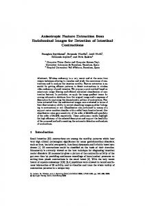
Without the loss of generality, it is assumed that σα = σr and D (.) = R(.) throughout the this paper. 2.2. Spectral-Spatial Feature Extraction Method Based on the PF As shown in Figure 1a, the cross-region mixture problem is quite common in HSIs. In particular, a lower spatial resolution increases the number of classes. As the ground sample distance increases, there is a potential for objects covered by a given pixel to be mixed [34]. Therefore, this paper presents the spectral-spatial feature extraction of the HSI algorithm based on the advantage that the PF can handle the cross-regional mixture problem [35]. As seen in Equations (1)–(6) and Figure 1b–d, the PF generates a new center pixel using a weighted summation of the neighbouring pixels in the HSI. The adjacent pixel t, center pixel s and pixel t − 1 in the neighbouring pixel set are all the same class, and the weight of pixel t is relatively larger. In Figure 1d, pixel t − 1 selected is close to the pixel t and points to the pixel t, where pixel s is in yellow, pixel t is in red, pixel t − 1 is in green. However, when there are mixed pixels in the neighbouring pixel sets, the weight of pixel t is smaller. Therefore, the PF ensures that the similar features of the same classes of pixels are enhanced, which suppresses the effects of cross-regional mixed pixels. Search window

Pixel t-1

Arbitrary pixel t

ωs,t = ωs,t−1 D(t − 1, tሻR(s, tሻ

Centre pixel s

t D(t − 1, tሻ=exp(

t-1 ωs,t−1

Generate

Neighbour set

R(s, tሻ=exp(

− Is −It 2 ሻ 2σ2r

t s

t-1

ωs,s = 1 s

(a)

− It−1 −It 2 ሻ 2σ2α

(b)

(c)

Output: O′s =

1 Zs

෌t∈N

s

ωs,t It

(d)

Figure 1. Flow diagram of HSI filtering using the PF. (a) Hyperspectral image (b) Neighbour pixel set Ns (c) the calculation of ωs,t and (d) the pattern for performing 2D filtering with w = 3 pixels.

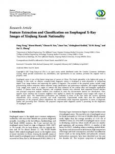
In addition, to improve the performance of the PF for feature extraction in HSIs, PCA is performed before filtering: the HSIs are reduced by PCA, and the redundant information between bands is greatly reduced in the updated pixels. However, although the HSIs lose a small amount of information after PCA, the bands are sorted according to the importance of the information. After the PF process, the increased effects of the important and reduced effects of the less important features are beneficial for feature extraction and in improving the classification accuracy. The specific process is shown in Figure 2. In the first step, PCA is used to reduce the dimensionality and remove the redundant inter-spectral information to obtain the principal components of an HSI. Then, the PCA feature is filtered with the PF. When cross-regional mixing occurs in the image, the filter template reduces or avoids the influence of cross-regional mixed pixels on the object pixel, thereby

Sensors 2018, 18, 1978

4 of 15

avoiding or effectively mitigating the effects of cross-regional mixed pixels. Through this technique, the proposed method can accurately extract the reflected spectral-spatial features of the real objects. Finally, to validate the effectiveness of the proposed method, experiments are carried out on HSIs using an SVM classifier trained on the learned spectral-spatial features. Algorithm 1 depicts the proposed HSI spectral-spatial feature extraction model based on the PF.

PF 1st feature PCA Dimension reduction

1st PF feature

2nd feature

2nd PF feature …

…

Hyperspectral image

SVM

PF

Classification result

PF

kth feature

kth PF feature

Figure 2. Schematic of the proposed PCA-PF-SVM method.

Algorithm 1: Specific flowchart of the spectral-spatial feature extraction algorithm based on the PF. Data: HSI I = ( I1 , I2 , · · · , In ) ∈ Rd×n , d is the number of HSI spectral bands, n is the number of pixels, the size of filter window is w, and the variance of the Gaussian function is σα (σr ). 0 0 0 0 Result: spectral-spatial feature O = (O1 , O2 , · · · , On ) ∈ Rk×n , k is the reduced dimension 1 The dimensionality of I is reduced from d to k using PCA, and the dimensionality-reduced HSI 0 0 0 0 is I = ( I1 , I2 , · · · , In ) ∈ Rk×n ; 2 for n = 1 : k do 3 Using Equation (6), calculate the pixel value distance between pixel s and pixel t; 4 Using Equation (5), calculate the pixel value distance between the pixel t and the pixel t − 1; 5 Using Equation (2), calculate the weight ωs,t of the pixel t in the adjacent set ; 0 6 Using Equation (1), calculate the pixel value Os of the pixel s output by the PF operation ; 7 end 0 0 0 0 k×n . 8 Output spectral-spatial feature O =(O1 , O2 , . . . On ) ∈ R 3. Experimental Settings In this paper, the training and testing samples for each HSI dataset were chosen randomly. In the experiments shown in Table 1, 20 label samples were randomly selected for each class as training samples, and the rest were used as test samples to verify the performance of the proposed methods in the three experiments. To verify the classification performance of different methods with sufficient training samples and insufficient training samples, in the experiments shown in Table 5, 10–50 training samples were selected from each class and the rest were used as test samples. For stability, each experiment was performed 10 times; the reported results are the averages.

Sensors 2018, 18, 1978

5 of 15

Table 1. Train-Test Distribution of sample for three datasets. Indian Pines

Salinas

University of Pavia

Class

Train

Test

Class

Train

Test

Class

Train

Test

Aifalfa Corn_n Corn_m Corn Grass_m Grass_t Grass_p Hay_w Oats Soybean_n Soybean_m Soybean_c Wheat Woods Buildings Stone

20 20 20 20 20 20 14 20 10 20 20 20 20 20 20 20

26 1408 810 217 463 710 14 458 10 952 2435 573 185 1245 366 73

weeds_1 weeds_2 fallow fallow_p fallow_s stubble Celery Grapes Soil Corn Lettuce_4 Lettuce_5 Lettuce_6 Lettuce_7 Vinyard_U Vinyard_T

20 20 20 20 20 20 20 20 20 20 20 20 20 20 20 20

1989 3706 1956 1374 2658 3939 3559 11,251 6183 3258 1048 1907 896 1050 7248 1787

Asphalt Meadows Gravel Trees Sheets Soil Bitumen Bricks Shadows

20 20 20 20 20 20 20 20 20

18,629 2079 3044 1325 5009 1310 3662 927 170

3.1. Dataset Description Three real HSI sets are used in this paper: the Indian Pines, Salinas and University of Pavia scenes. The Indian Pines image was obtained by the AVIRIS sensor and covers the northern agricultural Indian Pines test site. The image, which includes 16 categories of ground objects, contains 145 × 145 pixels, and only 200 out of all 224 bands are valid due to water absorption. The spatial resolution is 20 m per pixel, and the spectral range is 0.4 to 2.5 µm. The Salinas image contains 512 × 217 pixels and includes 16 types of ground objects at a 3.7-m spatial resolution and was acquired by the AVIRIS sensor over the Salinas Valley in California, USA. After removing 20 of the 224 bands due to noise and water absorption, the remaining 204 valid bands were utilized in the experiments. The University of Pavia image was acquired with 610 × 340 pixels at 1.3-m spatial resolution by the ROSIS Sensor in the city area around the University of Pavia. The image has a spectral range of 0.43 to 0.86 µm with 115 bands, where 12 bands that were noisy or impacted by water absorption were removed, and the remaining 103 bands were used. 3.2. Compared Algorithms In the experiments, the proposed classification method PCA-PF-SVM was compared to other widely used HSI classification methods, including SVM [11], PCA-SVM [36], PCA-Gabor-SVM [28], EPF-SVM [29], HiFi [30], LBP-SVM [37], R-VCANet-SVM [38] and PF-SVM. The parameters used for these methods were the default settings provided in the related literature. The source code for the algorithms was provided by the respective authors. The SVM classifier was based on the Libsvm library [39], and the optimal parameters of the SVM classifier were determined by a fivefold cross validation. The overall accuracy (OA), the average accuracy (AA), and the kappa coefficient are used to evaluate the performance of the methods. The OA indicates the probability that the classification results are consistent with the reference classification results. The AA refers to the mean of the percentage of correctly classified pixels for each class. The kappa coefficient is used for consistency check. 3.3. Parameter Sensitivity Analysis The proposed PCA-PF-SVM method has the following three important parameters: the filtering standard deviation σα (σr ), the filtering window size (w) and the feature dimension (k). To test the influence of the different parameter settings of the proposed model, we conducted extensive experiments were conducted on the Indian Pines scene. As shown in Figure 3a, the best OA, AA and

Sensors 2018, 18, 1978

6 of 15

kappa values were achieved when σα (σr ) = 1.5. In contrast, when σα (σr ) < 1.5, the accuracies decreased significantly because a small σα (σr ) leads to a smoother image. When σα (σr ) > 1.5, the classification accuracy remains relatively stable because the ability to suppress bad information improves after the filter parameter reaches a certain value. As shown in Figure 3b, the best OA, AA and kappa values were achieved when w = 8. These values are significantly lower when w < 8 because considerable important spatial information is lost when the window size is too small. Moreover, the values also decrease when w > 8 because the window contains a larger amount of irrelevant information that reduces the effect of the important spatial information and, thus, reduces the classification accuracy. From Figure 3c, OA becomes lager with the increase of PCA dimensions. When the dimension reaches to 45, OA trends to become decrease. In our experiments, k is set to 45 for the tradeoff between the computation complexity and classification accuracy. Therefore, in all of our experiments, the parameters were set as follows: σα (σr ) = 1.5, w = 8 and k = 45.

92

91 90.5 90 89.5 89 0.5

1 1.5 2 Standard deviation (  )

(a)

90

Overall accuracy (%)

Overall accuracy (%)

Overall accuracy (%)

91.5

88 86 84 82 80

91 90 89 88 87 86

10 20 30 Window size (w) (b)

85

20

40 60 Dimension (k) (c)

80

Figure 3. Indian Pines: analysis of the influence of parameters. (a) Standard deviation σα (σr ); (b) Window size w and (c) Dimension k.

3.4. Experimental Results (1) The proposed PCA-PF-SVM method has strong spatial capabilities. According to Figures 4–6 and Tables 2–4, the PCA-PF-SVM method achieves better OA, AA and kappa values than does the spectral classification method. The OA values based on the proposed PCA-PF-SVM method with respect to the Indian pines, Salinas and University of Pavia datasets are 36.14%, 8.87% and 17.78% higher, respectively, than the OA values based on the PCA-SVM method and 25.32%, 11.15% and 14.68% higher, respectively, than the OA values based on the SVM method. The main reason is that the spectral classification methods do not consider spatial information, while the method proposed in this paper fully considers spatial information. These results verify that the proposed method is effective in spectral-spatial feature extraction. (2) The results verify that combining PCA and the PF is effective for HSI feature extraction. Figures 4–6 and Tables 2–4 show that the PCA dimensionality reduction of the HSI does not improve the performance of the SVM classification and may even reduce the classification performance of the SVM. For example, the OA values of the PCA-SVM method for the Indian Pines dataset are lower than those for the SVM method. This result mainly occurs because although the PCA preserves the HSI’s main information, it also loses a small amount of information, thus affecting the SVM classification accuracy. However, the combination of PCA and the PF greatly enhances the performance. The OA values based on the proposed PCA-PF-SVM method for the Indian pines, Salinas and University of Pavia datasets are 13.26%, 3.42% and 7.86% higher, respectively, than are the OA values resulting the PF-SVM method. These experimental results show that it is necessary to apply PCA dimensionality reduction before filtering.

Sensors 2018, 18, 1978

7 of 15

Table 2. Classification accuracy of different methods on Indian Pines data set (%). Class

SVM

PCA-SVM

PCA-Gabor-SVM

PF-SVM

EPF-SVM

HiFi

LBP-SVM

R-VCANet-SVM

PCA-PF-SVM

Aifalfa Corn_n Corn_m Corn Grass_m Grass_t Grass_p Hay_w Oats Soybean_n Soybean_m Soybean_c Wheat Woods Buildings Stone

55.00 52.16 63.35 53.33 82.80 85.91 37.14 97.89 27.27 57.38 71.57 37.88 88.14 92.55 39.31 95.77

54.35 51.32 25.22 28.45 75.81 86.62 53.85 99.76 38.89 29.14 51.75 36.69 96.83 93.98 53.67 87.65

70.27 81.18 90.78 82.20 97.37 96.19 45.16 88.59 24.39 95.84 87.75 93.13 77.02 95.49 90.20 76.04

12.38 67.18 77.55 72.53 90.89 87.59 35.00 100.00 8.85 68.79 91.33 68.58 95.81 96.61 74.44 34.45

57.78 85.80 89.35 43.06 92.93 91.93 82.35 100.00 100.00 66.32 92.13 52.77 100.00 96.94 88.99 87.95

100.00 84.94 93.09 87.10 92.01 97.61 100.00 99.78 100.00 93.70 78.52 94.24 99.46 98.23 93.99 100.00

46.58 89.95 86.70 91.85 88.72 85.70 30.00 88.49 13.89 74.14 97.06 85.89 83.12 99.84 95.87 78.43

100.00 65.41 85.31 97.24 91.36 96.48 100.00 99.13 100.00 83.61 71.79 87.43 99.46 95.74 95.36 100.00

54.55 95.22 94.97 91.44 72.16 100.00 18.92 100.00 45.45 84.34 95.90 88.51 95.85 100.00 72.58 87.01

OA AA kappa

66.27±2.46 64.84 ± 2.28 0.62 ± 0.02

55.45 ± 4.38 60.25 ± 5.63 0.50 ± 0.04

88.99 ± 1.33 80.73 ± 1.60 0.87 ± 0.02

78.33 ± 1.69 67.62 ± 1.52 0.76 ± 0.02

83.03 ± 1.85 83.02 ± 3.19 0.81 ± 0.02

89.82 ± 2.01 94.54 ± 0.97 0.88 ± 0.02

88.70 ± 1.93 77.26 ± 2.58 0.87 ± 0.02

83.23 ± 1.75 91.77 ± 0.82 0.81 ± 0.01

91.59 ± 1.32 81.06 ± 3.91 0.90 ± 0.01

Table 3. Classification accuracy of different methods on Salinas data set (%). Class

SVM

PCA-SVM

PCA-Gabor-SVM

PF-SVM

EPF-SVM

HiFi

LBP-SVM

R-VCANet-SVM

PCA-PF-SVM

weeds_1 weeds_2 fallow fallow_p fallow_s stubble Celery Grapes Soil Corn Lettuce_4 Lettuce_5 Lettuce_6 Lettuce_7 Vinyard_U Vinyard_T

98.05 99.37 91.22 97.68 97.00 100.00 99.94 72.98 98.59 79.39 93.65 94.34 93.37 92.29 54.30 94.44

100.00 99.43 94.35 94.41 95.24 99.95 100.00 76.85 99.00 93.32 91.02 91.97 91.14 94.26 58.25 99.54

88.18 88.99 82.46 73.87 81.13 92.22 96.04 92.01 97.29 64.75 95.66 97.63 84.29 90.26 73.37 94.03

98.07 99.92 93.93 86.13 97.62 99.95 98.22 91.63 99.49 92.48 95.42 96.07 76.19 99.41 77.59 98.59

100.00 99.89 94.91 97.86 99.96 99.92 100.00 82.04 99.48 85.06 98.21 100.00 96.10 99.20 73.97 99.49

98.49 98.70 99.80 97.45 88.75 99.59 96.60 82.13 99.97 87.97 96.18 99.48 97.21 92.67 73.17 96.75

99.40 99.26 97.92 83.89 97.28 95.13 94.66 91.57 99.97 99.04 98.96 99.89 92.64 95.97 83.00 99.17

99.90 99.84 99.39 99.56 99.62 99.97 98.17 78.54 99.26 94.69 98.76 100.00 94.31 96.86 85.32 99.27

100.00 99.84 100.00 91.79 99.52 99.97 100.00 95.28 99.97 97.76 100.00 100.00 98.33 93.09 85.01 95.21

OA AA kappa

84.96 ± 1.17 91.04 ± 0.53 0.83 ± 0.01

87.24 ± 1.73 92.42 ± 0.93 0.86 ± 0.02

85.67 ± 1.99 87.01 ± 1.78 0.84 ± 0.02

92.69 ± 1.38 93.80 ± 0.85 0.92 ± 0.02

91.41 ± 2.29 95.38 ± 0.85 0.90 ± 0.03

90.50 ± 1.32 94.06 ± 0.68 0.89 ± 0.01

93.97 ± 2.28 95.48 ± 1.62 0.93 ± 0.03

91.58 ± 1.09 96.05 ± 0.40 0.91 ± 0.01

96.11 ± 0.86 97.24 ± 0.45 0.96 ± 0.01

Sensors 2018, 18, 1978

8 of 15

Table 4. Classification accuracy of different methods on University of Pavia data set (%). Class

SVM

PCA-SVM

PCA-Gabor-SVM

PF-SVM

EPF-SVM

HiFi

LBP-SVM

R-VCANet-SVM

PCA-PF-SVM

Asphalt Meadows Gravel Trees Sheets Soil Bitumen Bricks Shadows

87.52 91.00 61.72 70.10 98.42 46.04 54.64 80.23 100.00

82.14 90.51 39.42 79.54 100.00 53.61 32.06 57.68 99.35

72.39 95.96 75.01 40.27 88.21 68.69 78.94 80.20 49.44

85.47 97.60 56.17 80.30 99.25 70.30 71.72 60.79 83.23

98.05 97.40 89.16 96.20 95.05 64.27 58.20 76.20 99.89

80.40 89.74 82.92 83.64 99.17 89.72 96.79 92.55 99.46

84.36 97.98 72.93 51.19 86.32 75.02 76.85 78.43 45.34

79.96 83.39 88.12 96.75 100.00 93.57 99.01 88.39 100.00

92.30 99.47 84.96 76.68 99.92 84.80 85.61 79.43 96.95

OA AA kappa

75.73 ± 1.64 76.63 ± 1.43 0.69 ± 0.02

72.63 ± 3.40 70.48 ± 2.41 0.65 ± 0.04

76.58 ± 2.98 72.12 ± 2.81 0.70 ± 0.03

82.55 ± 3.41 78.31 ± 3.34 0.78 ± 0.04

87.00 ± 2.43 86.05 ± 2.39 0.83 ± 0.03

88.48 ± 1.90 90.49 ± 0.97 0.83 ± 0.02

81.82 ± 1.68 74.27 ± 2.19 0.76 ± 0.02

87.03 ± 1.19 91.17 ± 0.89 0.83 ± 0.01

90.41 ± 1.90 88.90 ± 2.05 0.89 ± 0.02

Table 5. Classification accuracy using varying numbers of training samples applied to three datasets. Indian Pines

Salinas

University of Pavia

Training Samples Perclass

Training Samples Perclass

Training Samples Perclass

Method

Quality Indexes

10

20

30

40

50

10

20

30

40

50

10

20

30

40

50

SVM

OA AA kappa

57.43 55.87 0.52

66.27 64.84 0.62

73.31 69.84 0.70

75.94 72.67 0.73

78.66 75.86 0.76

82.64 88.87 0.81

84.96 91.04 0.83

86.42 91.38 0.85

86.20 91.77 0.85

87.70 92.75 0.86

67.02 69.12 0.59

75.73 76.63 0.69

78.95 77.69 0.73

82.30 80.23 0.77

83.78 81.36 0.79

PCA-SVM

OA AA kappa

47.89 53.23 0.42

55.45 60.25 0.50

58.47 64.14 0.53

62.07 67.02 0.57

66.67 72.15 0.62

84.47 88.98 0.83

87.24 92.42 0.88

88.59 93.89 0.87

88.37 93.99 0.87

89.30 94.40 0.88

61.71 60.60 0.52

72.63 70.48 0.65

76.53 74.04 0.70

77.90 75.29 0.72

80.41 77.15 0.75

PCA-Gabor-SVM

OA AA kappa

76.03 75.90 0.73

88.99 80.73 0.87

93.06 86.93 0.92

94.64 88.79 0.94

96.09 91.78 0.96

73.62 76.95 0.71

85.67 87.01 0.84

89.29 90.49 0.88

93.08 93.70 0.92

94.46 94.91 0.94

65.51 63.76 0.57

76.58 72.12 0.70

81.26 77.19 0.76

84.30 80.11 0.80

86.18 83.28 0.82

PF-SVM

OA AA kappa

64.77 59.06 0.61

78.33 67.62 0.76

84.19 73.27 0.82

87.84 77.47 0.86

90.40 82.39 0.89

88.69 91.24 0.97

92.69 93.80 0.92

94.28 95.77 0.94

95.16 96.42 0.95

95.46 96.64 0.95

71.23 68.91 0.64

82.55 78.31 0.78

87.62 82.82 0.84

89.13 83.76 0.86

91.73 87.38 0.89

EPF-SVM

OA AA kappa

69.32 72.06 0.66

83.03 83.02 0.81

87.41 87.60 0.86

89.63 89.74 0.88

92.41 92.02 0.91

87.71 93.80 0.86

91.41 95.38 0.90

92.70 95.96 0.92

92.73 96.12 0.92

94.15 96.85 0.93

73.76 76.21 0.67

87.00 86.05 0.83

88.97 88.56 0.86

92.19 90.89 0.90

93.57 92.66 0.92

HiFi

OA AA kappa

81.08 89.44 0.79

89.82 94.54 0.88

91.65 95.74 0.91

93.63 96.36 0.93

93.44 96.72 0.93

86.53 92.08 0.85

90.50 94.06 0.89

92.08 95.47 0.91

92.67 96.20 0.92

93.59 96.76 0.93

81.83 85.40 0.77

88.48 90.49 0.83

88.64 91.91 0.85

90.22 92.99 0.87

90.94 93.58 0.88

LBP-SVM

OA AA kappa

80.49 70.96 0.78

88.70 77.26 0.87

92.01 83.29 0.91

94.85 86.72 0.94

95.58 87.00 0.95

89.65 90.41 0.89

93.97 95.48 0.93

96.18 96.13 0.96

96.86 96.88 0.97

97.91 97.87 0.98

70.35 66.39 0.63

81.82 74.27 0.76

85.75 81.33 0.82

89.39 84.85 0.86

90.34 86.41 0.87

R-VCANet-SVM

OA AA kappa

75.40 85.82 0.72

83.23 91.77 0.81

87.56 94.00 0.86

89.66 95.05 0.88

91.33 95.88 0.90

87.96 94.32 0.87

91.58 96.05 0.91

92.93 96.68 0.92

93.29 96.91 0.93

94.21 97.34 0.94

81.47 87.21 0.76

87.03 92.13 0.83

90.95 93.51 0.88

92.18 94.48 0.90

93.46 95.51 0.91

PCA-PF-SVM

OA AA kappa

84.20 78.28 0.82

91.59 81.06 0.90

94.32 87.29 0.94

95.23 89.65 0.95

96.55 92.22 0.96

93.91 96.04 0.93

96.11 97.24 0.96

96.83 98.28 0.96

97.84 98.70 0.98

98.45 99.14 0.98

85.14 83.17 0.81

90.41 88.90 0.89

91.62 88.26 0.89

94.12 91.80 0.92

95.34 93.41 0.94

Sensors 2018, 18, 1978

9 of 15

Ground truth image

SVM (OA=66.27%)

PCA-SVM (OA=55.45%)

PCA-Gabor-SVM (OA=88.99%)

EPF-SVM (OA=83.03%)

HiFi (OA=89.82%)

LBP-SVM (OA=88.7%)

R-VCANet-SVM (OA=83.23%)

PF-SVM (OA=78.33%)

PCA-PF-SVM (OA=91.59%)

Alfalfa

Corn_n

Corn_m

Corn

Grass_m

Grass_t

Grass_p

Hay_w

Oats

Soybean_n

Soybean_m

Soybean_c

Wheat

Woods

Buildings

Stone

Figure 4. The classification results of the Indian Pines image. Weeds_1

Weeds_2 Fallow Fallow_p Fallow_s Stubble

Celery

Ground truth image

SVM (OA=84.96%)

PCA-SVM (OA=87.24%)

PCA-Gabor-SVM (OA=85.67%)

PF-SVM (OA=92.69%)

Grapes Soil Corn Lettuce_4 Lettuce_5 Lettuce_6 Lettuce_7 Vinyard_U Vinyard_T

EPF-SVM (OA=91.41%)

HiFi (OA=90.50%)

LBP-SVM (OA=93.97%)

R-VCANet-SVM (OA=91.58%)

PCA-PF-SVM (OA=96.11%)

Figure 5. The classification results of the Salinas image.

Sensors 2018, 18, 1978

10 of 15

Asphalt Meadows Gravel Trees

Ground truth image

SVM (OA=75.73%)

PCA-SVM (OA=72.63%)

PCA-Gabor-SVM (OA=76.58%)

PF-SVM (OA=82.55%)

Metal sheets

Bare soil Bitumen Bricks Shadows

EPF-SVM (OA=87%)

HiFi (OA=88.48%)

LBP-SVM (OA=81.82%)

R-VCANet-SVM (OA=87.03%)

PCA-PF-SVM (OA=90.41%)

Figure 6. The classification results of the University of Pavia image.

(3) The proposed method is more effective than the other advanced classification methods. As shown in Figures 4–6 and Tables 2–4, compared with other methods, the PCA-PF-SVM method shows very good performance in terms of OA and kappa. On the Indian Pines, Salinas and University of Pavia datasets, the PCA-PF-SVM method shows more obvious effects than do the HiFi-We, LBP-SVM and R-VCANet-SVM methods. The OA values based on the proposed PCA-PF-SVM method for the Indian Pines, Salinas and University of Pavia datasets are 1.77%, 5.61% and 1.93% higher, respectively, than the OA values based on the HiFi-We method and 2.89%, 2.14% and 8.59% higher, respectively, than the OA values based on the LBP-SVM method and 8.36%, 4.53% and 3.38% higher, respectively, than the OA values based on the R-VCANet-SVM method. (4) The experimental results demonstrate the robustness of the proposed PCA-PF-SVM method. As shown in Figures 7–9 and Table 5, in both scenarios, as the number of training samples varies from 10 to 50, the proposed method achieves the highest OA. Its advantage is especially obvious when the number of training samples is small. For example, when the number of training samples per class is 10, our method has a 3.12–36.31% advantage on the Indian Pines image and a 3.5–20.29% advantage on the Salinas image and a 3.31–23.43% advantage on the University of Pavia image compared to the other methods. This is a highly meaningful result, because it means that a large number of non-labelled samples can be distinguished using a much smaller number of labelled samples, thus greatly improving the work efficiency, which further illustrates the robustness of the proposed method. (5) These experimental results show that the proposed method is useful for addressing the cross-regional mixture problems of HSIs. In Figure 10, the complete classified maps and ground truth maps obtained by PCA-PF-SVM are presented. The proposed method achieves better results on the cross-region mixture problem. For cross-region marked by white box in the three figures, PF can reduce cross-region problem, which keep better feature of image and improve further classification accuracy.

11 of 15

100

1

95

95

0.95

90 85 80 75 70

EPF-SVM HiFi LBP-SVM R-VCANet-SVM PCA-PF-SVM

90 85 80 75

EPF-SVM HiFi LBP-SVM R-VCANet-SVM PCA-PF-SVM

Kappa coefficient (%)

100

Average accuracy (%)

Overall accuracy (%)

Sensors 2018, 18, 1978

70 10 20 30 40 50 Training samples per class

65 10 20 30 40 50 Training samples per class

0.9 0.85 0.8 0.75 EPF-SVM HiFi LBP-SVM R-VCANet-SVM PCA-PF-SVM

0.7

0.65 10 20 30 40 50 Training samples per class

Figure 7. Influence of training samples on Indian Pines dataset.

96 94 92 90 EPF-SVM HiFi LBP-SVM R-VCANet-SVM PCA-PF-SVM

86 10 20 30 40 50 Training samples per class

98 96 94 92

EPF-SVM HiFi LBP-SVM R-VCANet-SVM PCA-PF-SVM

Kappa coefficient (%)

98

88

1

100

Average accuracy (%)

Overall accuracy (%)

100

0.95

0.9

0.85

90 10 20 30 40 50 Training samples per class

EPF-SVM HiFi LBP-SVM R-VCANet-SVM PCA-PF-SVM

10 20 30 40 50 Training samples per class

Figure 8. Influence of training samples on Salinas dataset. 95

90 85 80 75

EPF-SVM HiFi LBP-SVM R-VCANet-SVM PCA-PF-SVM

70 10 20 30 40 50 Training samples per class

1

Kappa coefficient (%)

95

Average accuracy (%)

Overall accuracy (%)

100

90

85

80

75 10

EPF HiFi-We LBP-ELM PCA-PF-SVM

20 30 40 50 Training samples per class

0.95 0.9 0.85 0.8 0.75 0.7 0.65

EPF-SVM HiFi LBP-SVM R-VCANet-SVM PCA-PF-SVM

10 20 30 40 50 Training samples per class

Figure 9. Influence of training samples on University of Pavia dataset.

(6) Statistical evaluation about the results: To further validate whether the observed increase in kappa is statistically significant, we use paired t-test to show the statistical evaluation about the results. T-test is popular in many related works [40–42]. We accept the hypothesis that the mean kappa of PCA-PF-SVM is larger than a compared method only if Equation (7) is valid:

√ ( a¯ − a¯ 2 ) n1 + n2 − 2 q 1 > t 1− α [ n 1 + n 2 − 2 ] ( n1 + n12 )(n1 s21 ) + n2 s22

(7)

1

where a¯ 1 and a¯ 2 are the means of kappa of PCA-PF-SVM and a compared method, s1 and s2 are the corresponding standard deviations, n1 and n2 are the number of realizations of experiments

Sensors 2018, 18, 1978

12 of 15

reported which is set as 10 in this paper. Paired t-test shows that the increases on kappa are statistically significant in all the three datasets (at the level of 95%), and it can be also observed in Figure 11.

(a)

(b)

(c)

(d)

(e)

(f)

(g)

(h)

(i)

Figure 10. Classification maps of PCA-BF-SVM methods on three datasets. (a,d,g) are false color composite image (R-G-B = band 50-27-17) for Indian Pines , University of pavia and Salinas datasets; (b,e,h) are ground truth classification results image; (c,f,i) are complete classified results image.

Sensors 2018, 18, 1978

13 of 15

0.9

0.9

0.95

0.8

0.9

0.7 0.6 0.5

kappa

kappa

kappa

0.8

0.7

0.6

0.85

0.8 1 2 3 4 5 6 7 8 9 method

0.4 1 2 3 4 5 6 7 8 9 method

(a) Indian Pine

1 2 3 4 5 6 7 8 9 method

(b) University of pavia

(c) Salinas

Figure 11. Box plot of kappa of different methods on three datasets. (a) Indian Pine (b) University of pavia (c) Salinas 1. SVM 2. PCA-SVM 3. PCA-Gabor-SVM 4. PF-SVM 5. EPF-SVM 6. HiFi 7. LBP-SVM 8. R-VCANet-SVM 9. PCA-PF-SVM. The center line is the median value, the edges of the box are the 25th and 75th percentiles, the whiskers extend to the most extreme points, and the abnormal outliers are plotted by “+”.

4. Conclusions The motivation for this study was to develop a simple feature extraction method to handle the cross-regional mixed problem of HSIs. The developed method extracts spectral-spatial features via the PF. However, the HSI’s high-dimensional problems affect the PF’s performance to a certain extent. To ensure a real effect, based on the characteristics of the HSI, PCA is used to reduce an images dimensions. Moreover, a combination PCA-PF feature extraction method is proposed. To evaluate the performance of the proposed method, three classical datasets with different complexities of cross-regional mixing problems were analyzed, and comparative experiments were also employed. The results show that the proposed method effectively solves the cross-regional mixture problem. In addition, feature extraction method in this paper use NRS and ELM for classification, and compares with PCA-Gabor-NRS and LBP-ELM.As shown in Table 6, classification results show that our method can obtain better results than that of the compared methods. Table 6. Classification Results obtained by PCA-Gabor-NRS, PCA-PF-NRS, LBP-ELM and PCA-PF-ELM. Indian Pines PCA-Gabor-NRS

PCA-PF-NRS

LBP-ELM

PCA-PF-ELM

Training Samples Perclass

OA

AA

kappa

OA

AA

kappa

OA

AA

kappa

OA

AA

kappa

10 20 30 40 50

68.46 82.56 88.93 91.99 93.71

61.32 75.63 83.28 87.17 89.21

0.65 0.80 0.87 0.91 0.93

84.50 90.82 93.73 94.79 95.72

76.99 83.84 87.69 89.67 90.08

0.83 0.90 0.93 0.94 0.95

80.89 88.37 92.57 94.42 95.76

89.16 93.62 96.09 96.76 97.77

0.79 0.87 0.92 0.94 0.95

83.15 91.44 94.35 95.69 97.08

90.43 95.32 96.81 97.68 98.37

0.81 0.90 0.94 0.95 0.97

Salinas PCA-Gabor-NRS

PCA-PF-NRS

LBP-ELM

PCA-PF-ELM

Training Samples Perclass

OA

AA

kappa

OA

AA

kappa

OA

AA

kappa

OA

AA

kappa

10 20 30 40 50

57.53 75.74 87.62 91.94 94.85

55.95 75.55 88.11 92.2 94.8

0.54 0.73 0.86 0.91 0.94

93.54 95.97 96.91 97.41 7.93

95.64 97.46 98.24 98.48 98.74

0.93 0.96 0.97 0.97 0.98

90.41 94.90 96.46 97.69 98.02

92.92 96.47 97.84 98.38 98.67

0.89 0.94 0.96 0.97 97.79

93.22 95.96 96.58 97.90 98.40

96.70 98.12 98.49 98.99 99.23

0.92 0.96 0.96 0.98 0.98

University of Pavia PCA-Gabor-NRS

PCA-PF-NRS

LBP-ELM

PCA-PF-ELM

Training Samples Perclass

OA

AA

kappa

OA

AA

kappa

OA

AA

kappa

OA

AA

kappa

10 20 30 40 50

50.86 63.07 69.39 76.64 82.26

51.76 62.57 67.65 75.21 81.09

0.41 0.55 0.62 0.71 0.78

80.73 89.18 93.06 94.48 95.21

78.73 86.87 91.04 92.77 93.73

0.75 0.86 0.91 0.93 0.94

73.98 82.47 86.52 88.83 90.77

76.15 82.9 86.42 87.93 90.36

0.67 0.78 0.82 0.85 0.88

82.18 89.42 91.13 92.69 94.60

82.47 89.09 91.26 92.52 93.42

0.77 0.86 0.88 0.90 0.93

Sensors 2018, 18, 1978

14 of 15

Author Contributions: Z.C. (Zhikun Chen) and Z.C. (Zhihua Cai) conceived and designed the experiments; Z.C. (Zhikun Chen) and J.J. performed the experiments; X.J. and X.F. analyzed the data; Z.C. (Zhikun Chen) wrote the paper. Funding: This work is partially supported by the National Natural Science Foundation of China under Grants 61773355 and 61403351 and 61402424, the Fundamental Research Funds for the Central Universities, China University of Geosciences (Wuhan), Qinzhou scientific research and technology development plan project (201714322). Acknowledgments: The authors would like to thank B. Pan, Y. Zhou, J.H.R. Chang, X. Kang and W. Li for providing the source code for their algorithms. Conflicts of Interest: The authors declare no conflicts of interest.

References 1. 2. 3. 4.

5. 6.

7. 8. 9. 10. 11. 12. 13. 14. 15. 16. 17. 18. 19. 20.

Jia, X.; Kuo, B.C.; Crawford, M.M. Feature mining for hyperspectral image classification. Proc. IEEE 2013, 101, 676–697. [CrossRef] Fauvel, M.; Tarabalka, Y.; Benediktsson, J.A.; Chanussot, J.; Tilton, J.C. Advances in spectral-spatial classification of hyperspectral images. Proc. IEEE 2013, 101, 652–675. [CrossRef] Han, Y.; Li, J.; Zhang, Y. Sea Ice Detection Based on an Improved Similarity Measurement Method Using Hyperspectral Data. Sensors 2017, 17, 1124. Wong, E.; Minnett, P. Retrieval of the Ocean Skin Temperature Profiles From Measurements of Infrared Hyperspectral Radiometers—Part II: Field Data Analysis. IEEE Trans. Geosci. Remote Sens. 2016, 54, 1891–1904. [CrossRef] Zhang, T.; Wei, W.; Zhao, B. A Reliable Methodology for Determining Seed Viability by Using Hyperspectral Data from Two Sides of Wheat Seeds. Sensors 2018, 18, 813. [CrossRef] [PubMed] Behmann, J.; Acebron, K.; Emin, D. Specim IQ: Evaluation of a New, Miniaturized Handheld Hyperspectral Camera and Its Application for Plant Phenotyping and Disease Detection. Sensors 2018, 18, 441. [CrossRef] [PubMed] Sandino, J.; Pegg, G.; Gonzalez, F. Aerial Mapping of Forests Affected by Pathogens Using UAVs, Hyperspectral Sensors, and Artificial Intelligence. Sensors 2018, 18, 944. [CrossRef] [PubMed] Ma, N.; Peng, Y.; Wang, S. An Unsupervised Deep Hyperspectral Anomaly Detector. Sensors 2018, 18, 693. [CrossRef] [PubMed] Jiang, J.; Ma, J.; Wang, Z.; Chen, C. Hyperspectral Image Classification in the Presence of Noisy Labels. IEEE Trans. Geosci. Remote Sens. 2018, 1, 99. Ma, J.; Jiang, J.; Zhou, H.; Zhao, J.; Guo, X. Guided Locality Preserving Feature Matching for Remote Sensing Image Registration. IEEE Trans. Geosci. Remote Sens. 2018. [CrossRef] Pal, M.; Foody, G. Feature Selection for Classification of Hyperspectral Data by SVM. IEEE Trans. Geosci. Remote Sens. 2010, 48, 2297–2307. [CrossRef] Huo, H.; Guo, J.; Li, Z. Hyperspectral Image Classification for Land Cover Based on an Improved Interval Type-II Fuzzy C-Means Approach. Sensors 2018, 18, 363. [CrossRef] [PubMed] Tong, F.; Tong, H.; Jiang, J.; Zhang, Y. Multiscale union regions adaptive sparse representation for hyperspectral image classification. Remote Sens. 2017, 9, 872. [CrossRef] Ma, J.; Jiang, J.; Liu, C.; Li, Y. Feature guided Gaussian mixture model with semi-supervised EM and local geometric constraint for retinal image registration. Inf. Sci. 2017, 417, 128–142. [CrossRef] Ma, J.; Chen, C.; Li, C.; Huang, J. Infrared and visible image fusion via gradient transfer and total variation minimization. Inf. Fusion 2016, 31, 100–109. [CrossRef] Ma, J.; Ma, Y.; Li, C. Infrared and visible image fusion methods and applications: A survey. Inf. Fusion 2019, 45, 153–178. [CrossRef] Jon, D.; David, M. Supervised Topic Models. Adv. Neural Inf. Process. Syst. 2008, 20, 121–128. Jiang, X.; Fang, X.; Chen, Z. Supervised Gaussian Process Latent Variable Model for Hyperspectral Image Classification. IEEE Geosci. Remote Sens. Lett. 2017, 14, 1–5. [CrossRef] Lee, H.; Kim, M.; Jeong, D. Detection of cracks on tomatoes using a hyperspectral near-infrared reflectance imaging system. Sensors 2014, 14, 18837–18850. [CrossRef] [PubMed] Kuo, B.; Li, C.; Yang, J. Kernel Nonparametric Weighted Feature Extraction for Hyperspectral Image Classification. IEEE Trans. Geosci. Remote Sens. 2009, 47, 1139–1155.

Sensors 2018, 18, 1978

21. 22. 23.

24. 25.

26. 27. 28. 29. 30. 31. 32. 33.

34. 35. 36. 37. 38. 39. 40. 41. 42.

15 of 15

Jolliffe, I. Principal Component Analysis, 2nd ed.; Springer: New York, NY, USA, 2002; Volume 98. Boukhechba, K.; Wu, H.; Bazine, R. DCT-Based Preprocessing Approach for ICA in Hyperspectral Data Analysis. Sensors 2018, 18, 1138. [CrossRef] [PubMed] Jiang, J.; Ma, J.; Chen, C.; Wang, Z.; Cai, Z.; Wang, L. SuperPCA: A Superpixelwise Principal Component Analysis Approach for Unsupervised Feature Extraction of Hyperspectral Imagery. IEEE Trans. Geosci. Remote Sens. 2018, doi:10.1109/TGRS.2018.2828029. [CrossRef] Song, Y.; Nie, F.; Zhang, C. A unified framework for semi-supervised dimensionality reduction. Pattern Recognit. 2008, 41, 2789–2799. [CrossRef] Chen, C.; Li, W.; Tramel, E.W.; Cui, M.; Prasad, S.; Fowler, J.E. Spectral–spatial preprocessing using multihypothesis prediction for noise-robust hyperspectral image classification. IEEE J. Sel. Top. Appl. Earth Obs. Remote Sens. 2014, 7, 1047–1059. [CrossRef] Chen, C.; Li, W.; Su, H.; Liu, K. Spectral-spatial classification of hyperspectral image based on kernel extreme learning machine. Remote Sens. 2014, 6, 5795–5814. [CrossRef] Jiang, J.; Chen, C.; Yu, Y. Spatial-Aware Collaborative Representation for Hyperspectral Remote Sensing Image Classification. IEEE Geosci. Remote Sens. Lett. 2017, 14, 404–408. [CrossRef] Li, W.; Du, Q. Gabor-Filtering-Based Nearest Regularized Subspace for Hyperspectral Image Classification. IEEE J. Sel. Top. Appl. Earth Obs. Remote Sens. 2014, 7, 1012–1022. [CrossRef] Kang, X.; Li, S.; Benediktsson, J. Spectral–Spatial Hyperspectral Image Classification With Edge-Preserving Filtering. IEEE Trans. Geosci. Remote Sens. 2014, 52, 2666–2677. [CrossRef] Pan, B.; Zhen, W.; Xu, X.j. Hierarchical Guidance Filtering-Based Ensemble Classification for Hyperspectral Images. IEEE Trans. Geosci. Remote Sens. 2017, 55, 4177–4189. [CrossRef] Zhou, Y.; Wei, Y. Learning Hierarchical Spectral-Spatial Features for Hyperspectral Image Classification. IEEE Trans. Cybern. 2016, 46, 1667–1678. [CrossRef] [PubMed] Wei, Y.; Zhou, Y.; Li, H. Spectral-Spatial Response for Hyperspectral Image Classification. Remote Sens. 2017, 9, 203. [CrossRef] Yu, S.; Liang, X.; Molaei, M. Joint Multiview Fused ELM Learning with Propagation Filter for Hyperspectral Image Classification. In Proceedings of the Asian Conference on Computer Vision, Taipei, Taiwan, 20–24 November 2016; pp. 374–388. Chang, J.; Wang, Y. Propagated image filtering. In Proceedings of the IEEE Conference on Computer Vision and Pattern Recognit, Boston, MA, USA, 7–12 June 2015; Volume 1, pp. 10–18. Li, J.; Bioucas-Dias, J.; Plaza, A. Spectral–Spatial Classification of Hyperspectral Data Using Loopy Belief Propagation and Active Learning. IEEE Trans. Geosci. Remote Sens. 2013, 51, 844–856. [CrossRef] Prasad, S.; Bruce, L. Limitations of Principal Components Analysis for Hyperspectral Target Recognition. IEEE Geosci. Remote Sens. Lett. 2008, 5, 625–629. [CrossRef] Li, W.; Chen, C.; Su, H.; Du, Q. Local Binary Patterns and Extreme Learning Machine for Hyperspectral Imagery Classification. IEEE Trans. Geosci. Remote Sens. 2015, 53, 3681–3693. [CrossRef] Pan, B.; Shi, Z.; Xu, X. R-VCANet: A New Deep-Learning-Based Hyperspectral Image Classification Method. IEEE J. Sel. Top. Appl. Earth Obs. Remote Sens. 2017, 10, 1975–1986. [CrossRef] Chang, C.; Lin, C. LIBSVM: A library for support vector machines. ACM Trans. Intell. Syst. Technol. (TIST) 2011, 2, 27. [CrossRef] Chen, Y.; Lin, Z.; Zhao, X.; Wang, G.; Gu, Y. Deep Learning-Based Classification of Hyperspectral Data. IEEE J. Sel. Top. Appl. Earth Obs. Remote Sens. 2017, 7, 2094–2107. [CrossRef] Pan, B.; Shi, Z.; Zhang, N.; Xie, S. Hyperspectral Image Classification Based on Nonlinear Spectral–Spatial Network. IEEE Geosci. Remote Sens. Lett. 2016, 13, 1782–1786. [CrossRef] Chen, Y.; Zhao, X.; Jia, X. Spectral–Spatial Classification of Hyperspectral Data Based on Deep Belief Network. IEEE J. Sel. Top. Appl. Earth Obs. Remote Sens. 2015, 8, 2381–2392. [CrossRef] c 2018 by the authors. Licensee MDPI, Basel, Switzerland. This article is an open access

article distributed under the terms and conditions of the Creative Commons Attribution (CC BY) license (http://creativecommons.org/licenses/by/4.0/).