Wavelet-based Feature Extraction From Oceanographic Images

IEEE TRANSACTIONS ON GEOSCIENCE AND REMOTE SENSING, VOL. 36, NO. 3, MAY 1998

767

Wavelet-Based Feature Extraction from Oceanographic Images Kiran K. Simhadri, S. S. Iyengar, Fellow, IEEE, Ronald J. Holyer, Matthew Lybanon, and John M. Zachary, Jr., Student Member, IEEE

Abstract—Features in satellite images of the oceans often have weak edges. These images also have a significant amount of noise, which is either due to the clouds or atmospheric humidity. The presence of noise compounds the problems associated with the detection of features, as the use of any traditional noise removal technique will also result in the removal of weak edges. Recently, there have been rapid advances in image processing as a result of the development of the mathematical theory of wavelet transforms. This theory led to multifrequency channel decomposition of images, which further led to the evolution of important algorithms for the reconstruction of images at various resolutions from the decompositions. The possibility of analyzing images at various resolutions can be useful not only in the suppression of noise, but also in the detection of fine features and their classification. This paper presents a new computational scheme based on multiresolution decomposition for extracting the features of interest from the oceanographic images by suppressing the noise. The multiresolution analysis from the median presented by Starck–Murtagh–Bijaoui [4], [5] is used for the noise suppression. Index Terms— Edge detection, feature extraction, image processing, multiresolution, noise suppression, wavelet transform.

I. INTRODUCTION

O

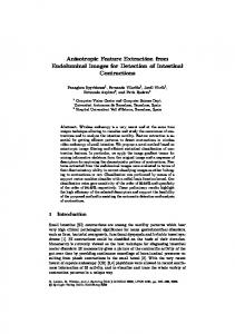
CEANOGRAPHERS desire accurate methods of tracking features in satellite images of the ocean to observe and quantify surface-layer dynamics. Infrared (IR) images of the ocean showing sea surface temperatures are widely used for the studies of this type. The satellite image in Fig. 1, which is typical of images used in these studies, is an infrared image of the northeast United States coastline, obtained from the Advanced Very High Resolution Radiometer (AVHRR) onboard the NOAA-7 satellite. Automatic feature tracking from time series of satellite IR images is problematic in two respects. First, the features of interest have low contrast (weak edges) and constantly evolving shapes from image to image. We define weak edges to be edges between adjacent regions with a small difference in grayscale intensity. Features merge, split, grow, shrink, Manuscript received October 5, 1995; revised December 3, 1996. This work was supported in part by ONR Grant N000014-92-J6003. K. K. Simhadri, S. S. Iyengar, and J. M. Zachary, Jr. are with the Robotics Research Laboratory, Department of Computer Science, Louisiana State University, Baton Rouge, LA 70803 USA (e-mail: [email protected]). R. J. Holyer and M. Lybanon are with the Naval Research Laboratory, Remote Sensing Division, Stennis Space Center, MS 39529 USA. Publisher Item Identifier S 0196-2892(98)01145-0.

Fig. 1. Infrared satellite image of the northeast United States coastline.

disappear, or are created on time scales that are comparable to the sampling interval of the satellite imager (typically, 12 h). In other words, the phenomenology under investigation is turbulent fluid flow, not rigid body motion. Therefore, tracking of ocean features is very difficult. The second problem, which results from the first, is that feature “motion” cannot be defined by a single set of values defining translation, rotation, and scaling. Different motions occur at different spatial scales, so that motion must be defined by parameters that are functions of scale as well as space and time. A simple example of different motions associated with different scales is seen in the ocean “front.” Most ocean fronts exhibit shear across the frontal boundary. Shear results in small lobes (shear instabilities) on the front that move along the frontal boundary. Concurrently, the entire frontal feature may be moving perpendicular to the boundary direction. This scenario results in small-scale and large-scale motions that are orthogonal. A feature tracking algorithm borrowed from rigid body problems will give a result that represents some unknown mixture of these two orthogonal motions. This combined motion has no physical meaning. Clearly, for the case of oceanographic images, an algorithm that resolves both motions is required. This paper deals with the wavelet-based feature extraction problem, which is the first step in a feature tracking problem, rather than directly addressing the feature tracking problem. Wavelets

0196–2892/98$10.00  1998 IEEE

768


(a)

(b)

Fig. 2. (a) Discrete wavelet transform. (b) Reconstructed image after suppressing noise.

have proven to be a useful technique for studying dynamic images [16], [17]. The wavelet transform, because it is able to localize the signal in both space and frequency [2], may be useful for addressing the problem of feature tracking in turbulent flow. For a broader treatment on this, see [1], [6], [13], and [15].

A. Motivation for Using Wavelets yields a meaThe Fourier transform of a function sure of the irregularities of the function in term of its high frequencies. However, this measure is not spatially localized, and hence, it is not possible to locate the position of the irregularity in the function. To get the information about the signal in time as well as frequency domains simultaneously, a windowed Fourier transform can be used. This transform obtains the irregularities of a function in a spatial region of a fixed size, and the function’s irregularities at various points are measured by translating the window back and forth on the spatial domain of the image. The main drawback of windowed Fourier transforms is that the spatial and frequency resolutions of the transform are fixed. A local feature such as edge cannot be located with a precision higher than the width of the window function . This limitation is inconvenient since a signal in general has features at arbitrary scales. In order to avoid this shortcoming, Mallat [2] defined the wavelet transform by decomposing the signal into a family of functions resulting from the translations and dilations of a single function called a wavelet. The wavelet transform can be generalized to any number of dimensions, but for the purpose of image processing, the twodimensional (2-D) case suffices. Wavelet transforms capture the features of images at all scales. Multiresolution decomposition involves decomposition of an image in frequency channels of constant bandwidth on a logarithmic scale. Wavelets and multiresolution transforms

Fig. 3. Computational architecture for proposed algorithm at one absolution level.

have been the focus of extensive study after the work on multiscale edge detection by Rosenfeld and Thurston [3]. Wavelets and multiresolution appear in the literature on image processing for a variety of applications, such as singularity detection [7], image coding using multiscale edges [8], [9], and feature detection [10]–[12], [15]. II. DISCRETE WAVELET TRANSFORM A. Mallat’s Wavelet Transform A discrete wavelet transform approach can be obtained from multiresolution analysis [2]. We reproduce the following development of Mallet [2]. A multiresolution analysis is a set of closed, nested subspaces generated by interpolations at different scales. A function is projected at each step onto the subset . This projection is defined by the scalar product of with the scaling function , which

SIMHADRI et al.: WAVELET-BASED FEATURE EXTRACTION FROM OCEANOGRAPHIC IMAGES

769

(a)

(b)

(c)

(d)

Fig. 4. Results of applying the new wavelet-based scheme proposed in this paper on northeast United States coastline image obtained on May 10 (a.m.). (a) Original image. (b) Edge image Ej at T = 3. (c) Edge image Ej +1 at T = 2. (d) Complementary image Wj +1 .

(1)

lost. The remaining information can be restored using the of in . The subspace complementary subspace can be generated by a suitable wavelet function with translation and dilation

(2)

(4)

is dilated and translated

is a scaling function that has the property

is a discrete low-pass filter associated with the where scaling function . Equation (2) permits the set to be computed directly from . If we start from the set , we compute all sets with without directly computing any other scalar product (3) At each step, the number of scalar products is divided by two. Step-by-step the signal is smoothed and information is

where

. We compute the scalar products with (5)

In order to restore the original data, Mallat uses the properties of orthogonal wavelets, but the theory has been generalized to a large class of filters [18]. Two other filter and , the conjugates of and , have been introduced [19], and the

770


(a)

(b)

(c)

(d)

Fig. 5. Results of applying the new wavelet-based scheme proposed in this paper on northeast United States coastline image obtained on May 10 (p.m.). (a) Original image. (b) Edge image Ej at T = 3. (c) Edge image Ej +1 at T = 2. (d) Complementary image Wj +1 .

restoration is performed with (6) This analysis can be easily extended to two dimensions. However, the 2-D algorithm is based on separate values leading to and directions being prioritized. This will lead to a nonisotropic analysis of the images, which is not an efficient way to extract fine features in the oceanographic images. B. Difficulties with Discrete Wavelet Transform The 2-D extension of Mallat’s algorithm leads to a wavelet transform with three wavelet functions [three wavelet coefficient subimages at each scale: Fig. 2(a)], which does not simplify the analysis and the interpretation of the wavelet coefficients for the reasons explained below. As the oceanographic images have fine features in all directions, an isotropic wavelet analysis seems more appropriate.

At a given scale, we derive a decimated number of wavelet coefficients. We cannot restore the intermediate values without using the approximation at this scale and the wavelet coefficients at smaller scales. Since the multiresolution analysis is based on scaling functions without a cutoff frequency, the application of the Shannon interpolation theorem is not possible. The interpolation of the wavelet coefficients can only be done after reconstruction and shift. This has no importance for signal coding, but the situation is not the same in a strategy in which we want to analyze or restore the image. By definition, the wavelet coefficient mean is null. Every time we have a positive structure at a scale, we have negative values surrounding it. These negative values often create artifacts during the restoration process or complicate the analysis. For instance, if we threshold small values (noise, nonsignificant structures, etc.) in the wavelet transform and reconstruct the image at the full resolution, the image becomes blurred [Fig. 2(b)].


771

(a)

(b)

(c)

(d)

Fig. 6. Results of applying the new wavelet-based scheme proposed in this paper on northeast United States coastline image obtained on May 11. (a) Original image. (b) Edge image Ej at T = 3. (c) Edge image Ej +1 at T = 2. (d) Complementary image Wj +1 .

C. Starck–Murtagh–Bijaoui Wavelet Transform The problems mentioned above led to the development of other multiresolution tools. Starck–Murtagh–Bijaoui [4], [5] modified the “a trous algorithm” and developed a new multiresolution approach using a morphological median filter. The algorithm is as follows. begin { with a size pixels. 1) Define a mask 2) Initialize to , and start from data . 3) med being the filtering median function, calculate med and median coefficients at scale by 4) If is less than the number of scales we want, return to 3). } end

The reconstruction is carried out by a simple addition of all scales (7) We use the above algorithm to suppress the noise in the image at various scales. III. SIMPLE EDGE DETECTION ALGORITHM Edge detection is an operation of locating the transition between two regions of distinct gray-level properties. Based on this observation, we present the following simple local edgedetection algorithm. begin { 1) Scan the image with a 3 3 empty window. 2) On each move of the window, calculate the , the maximum value in the window, and , the minimum value in the window.

772


(a)

(b)

(c)

(d)

Fig. 7. Results of applying the new wavelet-based scheme proposed in this paper on northeast United States coastline image obtained on May 11. (a) Original image. (b) Edge image Ej at T = 4. (c) Edge image Ej +1 at T = 3. (d) Complementary image Wj +1 .

3) If is less than the threshold , replace the central pixel with zero. Else move the window 4) The set of all nonzero points is the edge-detected image } end The specification of the threshold in the third step is the most sensitive part of this algorithm. The choice of the threshold (usually a number between zero and 255) depends on the image. Since the intensity changes occur at different scales in an image, their optimal detection requires the use of operators of different thresholds. We can define a multiresolution approach for edge detection at different scales. A multiresolution analysis is defined as a be the set of edges in closed nested set of subspaces. Let an image at the resolution , such that edge

(8)

(a) Fig. 8. Sobel edge-finding operators. (a)

(b)

Sh . (b) Sv .

where is the original image, is the threshold, and edge is the set of edges obtained using the above algorithm. As we increase the resolution (to a finer resolution) to and , where is the small number, the number of edges detected will increase as more and more fine edges can be detected. As we decrease the resolution, the number of edges detected will reduce. The information that is lost as we move to a coarser resolution can be restored using


(a)

773

(b)

(c) Fig. 9. Results of various edge-detecting methods on northeast United States coastline image obtained on May 10 (a.m.). (a) Sobel gradient operator. (b) Morphological gradient operator. (c) Result of our method.

the complementary subspace

of

in

IV. COMPUTATIONAL SCHEME

by (9)

This implies that the set of edges forms a sequence of nested subspaces satisfying the following conditions:

The reconstruction of the edges is then carried out by simple addition of all the scales (10) where is the set of edges at the “finest” scale and the set of edges at the “coarsest” scale.

is

FOR

FEATURE EXTRACTION

As mentioned earlier, feature extraction is the first step in a feature tracking algorithm, hence, it is important that the features have well-defined edges with the contour information well preserved. We present the following scheme to extract edge features from oceanographic images (Fig. 3). Step 1) Apply Starck–Murtagh–Bijaoui wavelet transform to the input image, and generate a wavelet plane. Step 2) Make all insignificant wavelet coefficients, i.e., all coefficients below a user-specified (often depends on the application) value, zero. Step 3) Reconstruct the image with the remaining coefficients. Step 4) Choose a threshold, and apply the edge-detection algorithm described in Section III. , Step 5) If the edges are not satisfactory decrement the threshold and go to Step 4).

774


(a)

(b)

(c)

(d)

(e)

(f)

Fig. 10. Results of thresholding on three different methods. Grayscale threshold value = 64. (a) Sobel gradient. (b) Morphological gradient. (c) Our method. Grayscale threshold value = 128. (d) Sobel gradient. (e) Morphological gradient. (f) Our method.

Such a scheme has several advantages over the discrete wavelet transform, as shown below. 1) Transform can be carried out using integer values leading to exact reconstructions at various scales as there will not be any errors due to roundoff. 2) Structure contours are preserved while the noise is suppressed. 3) The algorithm can be easily modified to work on intermediate scales (other than dyadic). V. EXPERIMENTAL RESULTS The test data consist of a set of six oceanographic images. We present results from four of them. Part (a) of Figs. 4–7 show the NOAA-7 images of the United States east coast, 12 h apart over a two-day period. In these images, bright areas represent warmer temperatures and dark areas represent the thermal colder temperatures. The Gulf Stream, warm eddies and cold eddies are important features, useful in understanding dynamic properties of oceanic systems. Fig. 4(b) shows the result of applying our method to obtain at a threshold . Even though an edge image the features of interest are visible in this image, the contour information is not fully preserved. The edges at the places where the contour information is missing are the edges that could not be detected at this resolution. We now go to a finer to . The resolution by decreasing the threshold contour information is fully preserved at this resolution, as can be seen from Fig. 4(c), which is the edge image at a “finer” resolution. The compromise that we make by obtaining finer detail in this image is more noise or extraneous features that are unimportant.

Since our ultimate goal is to track these features, it is difficult to distinguish features of importance from the other detail in the image. Fig. 4(d) shows the complementary image , which . This complementary of image in conjunction with the image at a coarser resolution can be used to estimate important parameters that can be used for feature tracking. For example, instead of working , image , which has less noise, can be used on image and, when at any point finer detail is required, the information . can be obtained from the complementary image Figs. 4–7 show the results of applying the proposed scheme to our sequence of four images. Parts (a)–(d) of each of the figures show the original image, edge image at a course resolution, edge image at a finer resolution, and the complementary image at the corresponding level, respectively. A. Comparison with Conventional Detectors In this section, we compare our method for detecting edges with two of the most frequently used conventional edge detectors: the Sobel edge operator and the morphological gradient edge detector. 1) Sobel Operator: The Sobel edge operator is a gradientbased method for edge detection that consists of two convolution kernels, as shown in Fig. 8. The kernel shown in Fig. 8(a) is sensitive to horizontal edges, while (b) is sensitive to vertical edges. Using these kernels, the gradient at a pixel can be approximated by . The output of the Sobel edge operator to one of our images is shown in Fig. 9(a). Notice how weakly the Sobel operator responds to the Gulf Stream and eddy edges. This weak response is a result of the smoothing effect of Sobel operators.


775

(a)

(b)

(c)

(d)

Fig. 11. Differences between images. (a) Sobel gradient image (threshold 64). (b) Sobel gradient image (threshold 128). (c) Morphological gradient image (threshold 64). (d) Morphological gradient image (threshold 128).

Similarly, erosion of a grayscale image element is defined as

Since the weak edges are similar to image noise, with respect to intensity, the Sobel gradient technique tends to smooth the weak edges along with the noise. 2) Morphological Operator: Another approach to edge detection involves a nonlinear method based on morphological filtering [14]. The dilation of a binary image by a structuring is defined as element

The morphological gradient, on an image , is determined from the dilation and erosion operators and is given by

(11)

(15)

The erosion of a binary image

by

is defined as (12)

The dilation of a grayscale image is defined as MAX

by a structuring element (13)

where and are the coordinates of a cell in whose center cell is the origin and is in the domain of .

MIN

by a structuring (14)

For details, see [13]. Fig. 9(b) shows the result of the morphological gradient operation with a 3 3 flat structuring element. As can be seen, only the main coastline features are extracted as strong edges in this operation. The reason for this can be attributed to the morphological operations used to perform the edge detection: erosion and dilation. Erosion removes small features, relative to the size of the structuring element, and dilation fills in gaps that meet the same criteria. The

776


(a)

(b)

(c) Fig. 12. Quantitative comparisons: (a) represents the fraction of pixels for different Sobel gradient thresholds in common with the images produced by our method, (b) is similarly defined for the morphological gradient method, and (c) is a graph showing the number of edge pixels for the three methods at different threshold values.

weak edges that form much of the structure in the currents and eddies happen to meet this criteria. Threshold images indicate the signal strength of the weak edges for the three methods being compared. Fig. 10 presents two sets of images for two different grayscale threshold values (64 and 128). Each threshold image is determined from Fig. 9(a)–(c). Fig. 10 highlights the advantage our method has in extracting weak edges from images. The Sobel gradient method in Fig. 10(a) does not preserve the smaller structure associated with eddies and currents ancillary to the main current stream to the east of the coastline. The morphological gradient method in Fig. 10(b) is even worse in this respect. However, the results of our method in Fig. 10(c) for the same grayscale threshold value show that, in addition to the more prominent oceanographic structure, finer structure associated with smaller currents and eddies are preserved. The same effect is demonstrated in Fig. 10(d)–(f) for a larger threshold value of 128 , although as the threshold value is increased, structure is removed from the image in all cases. We have observed the retention of fine oceanographic detail by our wavelet-based

method for threshold values across the entire intensity interval . Using the threshold images computed from the three different methods, difference images are presented in Fig. 11(a) and (d). The light grayscale values isolated along the edges representing the coastline are pixels that are in either the Sobel gradient images or morphological gradient images and not in the image produced by our wavelet-based method. The darker grayscale values, which can determine much of the finer oceanographic detail when compared to Fig. 9(a) and (c), represent edge pixels that are in images produced by our method and not in the images produced by either the Sobel gradient operator or the morphological gradient operator (again, depending on the image under observation). As mentioned, these so-called difference images clearly show the smaller oceanographic detail captured by our method, which correspond to weak edges in the original satellite image but not captured by the other two methods. The graphs in Fig. 12(a)–(c) show quantitative relationships between our wavelet-based method, the Sobel gradient


Fig. 13.

Qualitative comparison.

777

values compared to the Sobel gradient and morphological gradient edge-detection techniques. The same concept of multiresolution decomposition can be extended to address dynamic tracking of these features from time series images, but then the decomposition has to be not only in the spatial domain, but also in the time domain. REFERENCES

method, and the morphological gradient method. Fig. 12(a) shows the behavior of the fraction of pixels in the image produced by the Sobel gradient method, which are in common with our method across the possible threshold values. For low threshold values ( 125), a high percentage of the pixels in the image produced by the Sobel operator are in common with the image produced by our method. However, as the threshold increases, this percentage decreases markedly. The interpretation is that weak edges are not filtered out at low threshold values in the Sobel gradient images, but since they are weakly represented, they are removed as the threshold value increases. On the other hand, our method preserved the weak edges across a wide interval of threshold values. This is advantageous if the weak edges represent interesting structures, and they do in these oceanographic images. Hence, there appears to exist an element of stability across threshold values for weak edges in our method. Except for sharp discontinuities at threshold values 32 and 225, the percentage of pixels, with respect to the morphological gradient images, in common with the images produced by our method remains relatively constant around 43% [as shown in Fig. 12(b)]. Tests show that this number depends on the nature of the structuring element used in the dilation and erosion operators of the morphological gradient method as well as in the wavelet coefficients of our method. Fig. 12(c) presents the number of edge pixels in threshold images for each of the three methods. The number of edge pixels in the Sobel gradient and morphological gradient methods drops suddenly for low threshold values, which implies and is supported by viewing the loss of weak edges. The decrease in edge pixel count is not as sudden for our method, and the count remains relatively stable and greater than the other methods until the threshold value becomes quite large ( 150 for the Sobel gradient method.) Also, note that for a threshold value of one, the Sobel and morphological gradient methods have an extremely high number of edge pixels (perhaps this is a result of capturing noise in the images). However, as seen from the graph, our method captures the same level of detail for threshold values from one to around 70, further substantiating our claim of edge-detection stability. A qualitative comparison of the Sobel gradient and morphological gradient methods with our wavelet-based method is summarized in Fig. 13.

[1] B. Jawerth and W. Sweldens, “An overview of wavelet based multiresolution analyzes,” SIAM Rev., vol. 36, pp. 377–412, Sept. 1994. [2] S. Mallat, “A theory of multiresolution signal decomposition: The wavelet representation,” IEEE Trans. Pattern Anal. Machine Intell., PAMI-11, vol. 7, pp. 674–693, July 1989. [3] A. Rosenfeld and M. Thurston, “Edge and curve detection for visual scene analysis,” IEEE Trans. Comput., vol. C-20, pp. 562–569, June 1971. [4] J. L. Starck, F. Murtagh, and A. Biajaou, “Image restoration with noise suppression using a wavelet transform and a multiresolution support constraint,” in Proc. SPIE, Image Reconstruct. Restorat., vol. 2302, T. J. Schulz and D. L. Snyder, Eds. Bellingham, WA: SPIE, 1994, pp. 132–143. , “Multiresolution and astronomical image processing,” Astro[5] nomical Data Analysis Software and Systems IV, D. Shaw, H. Payne, and J. Hayes, Eds. New York: ASP, 1994. [6] A. Graps, “An introduction to wavelets,” IEEE Computat. Sci. Eng. Mag., to be published. [7] S. Mallat and W. L. Hwang, “Singularity detection and processing with wavelets,” IEEE Trans. Inform. Theory, vol. 38, pp. 617–643, Mar. 1992. [8] S. Mallat and S. Zhong, “Characterization of signals from multiscale edges,” IEEE Trans. Pattern Anal. Machine Intell., vol. 7, pp. 710–732, July 1992. [9] J. Froment and S. Mallat, “Second generation compact image coding with wavelets,” Wavelets: A Tutorial in Theory and Applications. New York: Academic, pp. 655–678, 1992. [10] J.-S. Lee, Y.-N. Sun, C.-H. Chen, and C.-T. Tsai, “Wavelet based corner detection,” Pattern Recognit., vol. 26, no. 6, pp. 853–865, 1993. [11] S. A. Little, P. H. Carter, and D. K. Smith, “Wavelet analysis of bathymetric file reveals anomalous crust,” Geophys. Res. Lett., vol. 20, pp. 1915–1918, Sept. 1992. [12] J. G. Teti and H. N. Kritikos, “SAR ocean image representation using wavelets,” IEEE Trans. Geosci. Remote Sensing, vol. 30, pp. 1089–1094, Sept. 1992. [13] S. Krishnamurthy, S. S. Iyengar, R. J. Holyer, and M. Lybanon, “Histogram based morphological edge detector,” IEEE Trans. Geosci. Remote Sensing, vol. 32, pp. 759–767, July 1994. [14] J. Serra, Image Analysis and Mathematical Morphology. New York: Academic, 1982. [15] L. Prasad and S. S. Iyengar, Wavelet Analysis with Applications to Image Processing. Boca Raton, FL: CRC, June, 1997. [16] Y. Meyer, Ondelettes et Opérateurs, I: Ondelettes, II: Opératuers de Calderón-Zygmund, III: (with R. Coifman) Opérateurs multilinéaires. Paris, France: Hermann, 1990 (English translation of the first volume is published by Cambridge, U.K.: Cambridge Univ. Press). [17] Y. Meyer, “Ondelettes sur l’intervalle,” Rev. Mat. Iberoamericana, vol. 7, pp. 115–133, 1992. [18] A. Cohen, I. Daubechies, and J. Feauveau, “Bi-orthogonal bases of compactly supported wavelets,” Commun. Pure Appl. Math., vol. 45, pp. 485–560, 1992. [19] I Daubechies, “Ten lectures on wavelets,”CBMS-NSF Region. Conf. Series Appl. Math., SIAM, Philadelphia, PA, 1992, vol. 61.

VI. CONCLUSION We have described a new computational scheme for extracting fine edges from the oceanographic images. The scheme was based on multiresolution decomposition of images. This scheme yields defined edge features and exhibits stable edge-preserving behavior across threshold

Kiran K. Simhadri received the M.S. degree in system science from Louisiana State University, Baton Rouge, in 1995. He is a Software Engineer for a company related to General Electric Company, WI. His research areas of interest image processing, computer vision and pattern recognitions.

778


S. S. Iyengar (M’88–SM’89–F’95) received the Ph.D. degree in 1974. He is Chairman and Professor of the Computer Science Department, Louisiana State University (LSU), Baton Rouge. He has been actively involved in research in high-performance algorithms. He has served as a Principal Investigator on research projects supported by the Office of Naval Research, National Science Foundation, NASA, The United States Army Research Office, DOE, Naval Research Laboratory, Jet Propulsion Laboratory (JPL), and various state agencies and has served as a Consultant to many government agencies as well as in private industry. He has been a Visiting Professor/Scientist at JPL, ORNL, and the Indian Institute of Science. He has made significant contributions and published in the areas of high-performance algorithms in image processing, sensor fusion, parallel models of computation for a variety of applications, computational aspects of motion planning, and vision problems. He has published over 220 papers and has authored or coauthored several textbooks for Prentice-Hall, CRC Press, and others. His edited books have appeared in publications of the IEEE Computer Society Press and Ablex. He has supervised over 29 Ph.D. dissertations and 60 M.S. projects and theses at LSU. Many of his former students presently hold positions at national research labs, including JPL, ORNL, and Los Alamos, as well as university teaching positions. Dr. Iyengar is a Distinguished Visitor of the IEEE, a member of the New York Academy of Sciences, and was an ACM National Lecturer from 1985 to 1995. He was selected to be on the prestigious NIH-NLM review committee in the area of medical informatics in 1993 for a four-year term. He is a winner of the 1997 IEEE Technical Achievement Award for Outstanding Contributions to Image Data Structures and Sensor/Signal Fusion. In 1996, he was awarded the LSU Distinguished Faculty Award for excellence in research and the Tiger Athletic Foundation Teaching Award. He has been a Guest Editor for the IEEE TRANSACTIONS ON COMPUTERS, IEEE TRANSACTIONS ON DATA AND KNOWLEDGE ENGINEERING, IEEE TRANSACTIONS ON SYSTEMS MANUFACTURING, IEEE TRANSACTIONS ON SOFTWARE ENGINEERING, Journal of Theoretical Computer Science, Journal of Computers and Electrical Engineering, and the Journal of the Franklin Institute, and he is a Series Editor for Neurocomputing of Complex Systems.

Ronald J. Holyer received the B.A. degree in physics and mathematics from Augustana College, Sioux Falls, SD, in 1964, the M.S. degree in physics from the South Dakota School of Mines and Technology, Rapid City, in 1966, and the Ph.D. degree in geology from the University of South Carolina, Columbia, in 1989. He is Head of the Computer Sciences and Physics Section, Remote Sensing Applications Branch, Naval Research Laboratory, Stennis Space Center, MS. His interests are image processing, pattern recognition, and automated image interpretation.

Matthew Lybanon received the B.S. and M.S. degrees in physics from the Georgia Institute of Technology, Atlanta, in 1960 and 1962, respectively. He is currently with the Remote Sensing Applications Branch of the Naval Research Laboratory, Stennis Space Center, MS. His current research interests include expert systems, generalized nonlinear least squares methods, genetic algorithms, image processing, mathematical morphology, and applications of those topics to the extraction of information on ocean dynamics and sea ice from satellite observations. Mr. Lybanon is a member of the American Geophysical Union, American Physical Society, and American Association of Physics Teachers.

John M. Zachary, Jr. (S’97) received the B.S. degree in computer science from Louisiana State University (LSU), Baton Rouge, in 1994. He is presently pursuing the Ph.D. degree at LSU. He was a Visiting Research Associate at the NASA Jet Propulsion Laboratory, Pasadena, CA, and spent a year at the University of Alabama at Birmingham. His research interests include content-based image retrieval, computer vision, neural networks, and global optimization. Mr. Zachary is a student member of ACM, AAAI, and SPIE.