Spectrum of a class of matrices and its applications

Spectrum of a class of matrices and its applications∗

arXiv:1612.00648v1 [math.CO] 2 Dec 2016

Lihua You

†

Man Yang

‡

Jinxi Li§

Liyong Ren¶

School of Mathematical Sciences, South China Normal University, Guangzhou, 510631, P.R. China

Abstract In this paper, we give the spectrum of a matrix by using the quotient matrix, then we apply this result to various matrices associated to a graph and a digraph, including adjacency matrix, (signless) Laplacian matrix, distance matrix, distance (signless) Laplacian matrix, to obtain some known and new results. Moreover, we propose some problems for further research. AMS Classification: 05C50, 05C35, 05C20, 15A18 Keywords: Matrix; Quotient matrix; Graph; Digraph; Spectrum; Spectral radius

1

Introduction We begin by recalling some definitions. Let M be an n × n matrix, λ1 , λ2 , . . . , λn be the

eigenvalues of M. It is obvious that the eigenvalues may be complex numbers since M is not symmetric in general. We usually assume that |λ1 | ≥ |λ2 | ≥ . . . ≥ |λn |. The spectral radius of M is defined as ρ(M) = |λ1 |, i.e., it is the largest modulus of the eigenvalues of M. If

M is a nonnegative matrix, it follows from the Perron-Frobenius theorem that the spectral radius ρ(M) is a eigenvalue of M. If M is a nonnegative irreducible matrix, it follows from the Perron-Frobenius theorem that ρ(M) = λ1 is simple. Let G be a connected graph with vertex set V (G) and edge set E(G). Let A(G) = (aij ) denote the adjacency matrix of G, where aij is equal to the number of edges vi vj . The ∗

L. You’s research is supported by the Zhujiang Technology New Star Foundation of Guangzhou (Grant No. 2011J2200090) and Program on International Cooperation and Innovation, Department of Education, Guangdong Province (Grant No.2012gjhz0007). † Corresponding author: [email protected]. ‡ Email address: [email protected]. § Email address: [email protected]. ¶ Email address: [email protected].

1

spectral radius of A(G), denoted by ρ(G), is called the spectral radius of G. Let diag(G) = diag(d1, d2 , . . . , dn ) be the diagonal matrix with degree of the vertices of G and Q(G) = diag(G) + A(G) be the signless Laplacian matrix of G, L(G) = diag(G) − A(G) be the

Laplacian matrix of G. The spectral radius of Q(G), denoted by q(G), is called the signless

Laplacian spectral radius of G. The spectral radius of L(G), denoted by µ(G), is called the Laplacian spectral radius of G. For u, v ∈ V (G), the distance between u and v, denoted by dG (u, v) or duv , is the length

of the shortest path connecting them in G. For u ∈ V (G), the transmission of vertex u in G

is the sum of distances between u and all other vertices of G, denoted by T rG (u).

Let G be a connected graph with vertex set V (G) = {v1 , v2 , . . . , vn }. The distance matrix

of G is the n × n matrix D(G) = (dij ) where dij = dvi vj . The distance spectral radius of G,

denoted by ρD (G), is the spectral radius of D(G), which is the largest eigenvalue of D(G).

In fact, for 1 ≤ i ≤ n, the transmission of vertex vi , T rG (vi ) is just the i-th row sum of

D(G). Let T r(G) = diag(T rG (v1 ), T rG (v2 ), . . . , T rG (vn )) be the diagonal matrix of vertex transmission of G. M. Aouchiche and P. Hansen [1] introduced the Laplacian and the signless

Laplacian for the distance matrix of a connected graph. The matrix L(G) = T r(G) − D(G) is called the distance Laplacian of G, while the matrix Q(G) = T r(G) + D(G) is called the

distance signless Laplacian matrix of G. It is obvious that Q(G) is irreducible, nonnegative,

symmetric and positive semidefinite. The distance signless Laplacian spectral radius of G,

denoted by q D (G), is the spectral radius of Q(G), which is the largest eigenvalue of Q(G).

The spectral radius of L(G), denoted by µD (G), is called the distance Laplacian spectral radius of G.

Since G is a connected graph, then A(G), Q(G), D(G) and Q(G) are nonnegative irre-

ducible matrices, it follows from the Perron Frobenius Theorem that ρ(G), q(G), ρD (G) and

q D (G) are real numbers and there is a positive unit eigenvector corresponding to ρ(G), q(G), ρD (G) and q D (G), respectively. → − → − → − → − − → Let G = (V ( G ), E( G )) be a digraph, where V ( G ) = {v1 , v2 , . . . , vn } and E( G ) are → − → − the vertex set and arc set of G , respectively. A digraph G is simple if it has no loops and → − → − multiple arcs. A digraph G is strongly connected if for every pair of vertices vi , vj ∈ V ( G ), there are directed paths from vi to vj and from vj to vi . In this paper, we consider finite,

simple strongly connected digraphs. → − Let G be a digraph. If two vertices are connected by an arc, then they are called adjacent. → − For e = (vi , vj ) ∈ E( G ), vi is the tail (the initial vertex) of e, vj is the head (the terminal 2

vertex) of e. → − → − → − → − − + Let N− → (vi ) = {vj ∈ V ( G )|(vj , vi ) ∈ E( G )} and N− → (vi ) = {vj ∈ V ( G )| (vi , vj ) ∈ E( G )} G

G

denote the in-neighbors and out-neighbors of vi , respectively. → − → − → − For a digraph G , let A( G ) = (aij ) denote the adjacency matrix of G , where aij is equal → − → − to the number of arcs (vi , vj ). The spectral radius of A( G ), denoted by ρ( G ), is called the → − spectral radius of G . → − + + Let diag( G ) = diag(d+ 1 , d2 , . . . , dn ) be the diagonal matrix with outdegree of the vertices → − → − → − → − → − → − → − of G and Q( G ) = diag( G )+A( G ) be the signless Laplacian matrix of G , L( G ) = diag( G )− → − − → → − → − A( G ) be the Laplacian matrix of G . The spectral radius of Q( G ), ρ(Q( G )), denoted by → − → − q( G ), is called the signless Laplacian spectral radius of G .

→ (u, v) or duv , is the length of For u, v ∈ V (G), the distance from u to v, denoted by d− G → − → − the shortest directed path from u to v in G . For u ∈ V ( G ), the transmission of vertex u in → − → − → (u). G is the sum of distances from u to all other vertices of G , denoted by T r− G → − → − Let G be a connected digraph with vertex set V ( G ) = {v1 , v2 , . . . , vn }. The distance → − → − → (vi , vj ). The distance spectral matrix of G is the n × n matrix D( G ) = (dij ) where dij = d− G → − → − → − D radius of G , denoted by ρ ( G ), is the spectral radius of D( G ).

→ (vi ) is just the i-th row sum of In fact, for 1 ≤ i ≤ n, the transmission of vertex vi , T r− G − → → − → (vn )) be the diagonal matrix of vertex → (v2 ), . . . , T r− → (v1 ), T r− D( G ). Let T r( G ) = diag(T r− G G G → − → − transmission of G . The distance signless Laplacian matrix of G is the n × n matrix defined

similar to the undirected graph by Aouchiche and Hansen as − → → − → − Q( G ) = T r( G ) + D( G ).

→ − → − → − → − Let L( G ) = T r( G ) − D( G ) be the distance Laplacian matrix of G . The distance signless → − → − → − → − Laplacian spectral radius of G , ρ(Q( G )), denoted by q D ( G ), is the spectral radius of Q( G ). → − → − → − → − − → Since G is a simple strongly connected digraph, then A( G ), Q( G ), D( G ) and Q( G ) are → − nonnegative irreducible matrices. It follows from the Perron Frobenius Theorem that ρ( G ), → − → − → − → − → − ρ(Q( G )) = q( G ), ρD ( G ) and ρ(Q( G )) = q D ( G ) are positive real numbers and there is a → − → − → − → − positive unit eigenvector corresponding to ρ( G ), q( G ), ρD ( G ) and q D ( G ), respectively. For a connected graph G = (V (G), E(G)), the vertex connectivity of a graph denoted by κ(G), is the minimum number of vertices whose deletion yields the resulting graph disconnected. Clearly, let G be a connected graph on n vertices, then 1 ≤ κ(G) ≤ n − 1. → − → − → − Similarly, for a strongly connected digraph G = (V ( G ), E( G )), the vertex connectivity of → − a digraph denoted by κ( G ), is the minimum number of vertices whose deletion yields the 3

→ − resulting digraph non-strongly connected. Clearly, let G be a strongly connected digraph → − with n vertices, then 1 ≤ κ( G ) ≤ n − 1. There are many literatures about graphs’ and digraphs’ connectivity. For early work, see

[27], Ye-Fan-Liang characterize the graphs with the minimal least eigevalue among all graphs with given vertex connectivity or edge connectivity. In 2010, Ye-Fan-Wang [28] characterize the graphs with maximum signless Laplacian or adjacency spectral radius among all graphs with fixed order and given vertex or edge connectivity. Liu [24] characterized the minimal distance spectral radius of simple connected graphs with given vertex connectivity, or matching number, or chromatic number, respectively. Brualdi [4] wrote a stimulating survey on this topic. In 2012, Lin-Shu-Wu-Yu [20] establish some upper or lower bounds for digraphs with some given graph parameters, such as clique number, girth, and vertex connectivity, and characterize the corresponding extremal graphs, give the exact value of the spectral radii of those digraphs. Besides, Lin-Yang-Zhang-Shu [22] characterize the extremal digraphs (graphs) with minimum distance spectral radius among among all digraphs (graphs) with given vertex (edge) connectivity. In 2013, Lin-Drury [18] characterize the extremal digraphs which attain the maximum Perron root of digraphs with given arc connectivity and number of vertices. Lin-Shu [21] determine the extremal digraph with the minimal distance spectral radius with given arc connectivity. Xing-Zhou [26] determine the graphs with minimal distance signless Laplacian spectral radius among the connected graphs with fixed number of vertices and connectivity. Oscar Rojo and Eber Lenes [25] obtained a sharp upper bound on the incidence energy of graphs in terms of connectivity. Furthermore, some upper or lower bounds were obtained by the outdegrees and the average 2-outdegrees [6, 11]. In 2014, Hong-You [13] determine the digraphs with maximal signless Laplacian spectral radius among the strongly connected digraphs with given vertex connectivity. On the other hand, some extremal digraphs which attain the maximum or minimum spectral radius, the signless Laplacian spectral radius, the distance spectral radius, or the distance signless Laplacian spectral radius of digraphs with given parameters, such as given vertex connectivity, given arc connectivity, given dichromatic number, given clique number, given girth and so on, were characterized, see e.g. [18, 21, 20, 22, 26]. In this paper, we give the spectrum of a matrix using the quotient matrix, and also apply these results to various matrices associated with graphs and digraphs as mentioned above.

4

Some know results are improved.

2

Some preliminaries

Definition 2.1. ([3, 14]) Let A = (aij ), B = (bij ) be n × n matrices. If aij ≤ bij for all i and j, then A ≤ B. If A ≤ B and A 6= B, then A < B. If aij < bij for all i and j, then A ≪ B.

Lemma 2.2. ([3, 14]) Let A, B be n × n matrices with the spectral radius ρ(A) and ρ(B).

If 0 ≤ A ≤ B, then ρ(A) ≤ ρ(B). Furthermore, if B is irreducible and 0 ≤ A < B, then ρ(A) < ρ(B). By Lemma 2.2, we have the following results in terms of digraphs. → − → − → − Corollary 2.3. Let G be a digraph and H be a spaning subdigraph of G . Then → − → − → − → − (i) ρ( H ) ≤ ρ( G ), q( H ) ≤ q( G ). − → → − → − → − → − (ii) If G is strongly connected, and H is a proper subdigraph of G , then ρ( H ) < ρ( G ), → − → − q( H ) < q( G ). → − → − → − → − → − → − (iii) If G and H are strongly connected, then ρD ( H ) ≥ ρD ( G ), q D ( H ) ≥ q D ( G ). − → → − → − → − → − → − (iv) If H is a proper subdigraph of G , then ρD ( H ) > ρD ( G ), q D ( H ) > q D ( G ). The theorem for undirected graph is also established. Lemma 2.4. ([3]) If A is an n × n nonnegative matrix with the spectral radius ρ(A) and row

sums r1 , r2 , . . . , rn , then min ri ≤ ρ(A) ≤ max ri . Moreover, if A is irreducible, then one of 1≤i≤n

1≤i≤n

the equalities holds if and only if the row sums of A are all equal.

←→ ←→ ←→ ←→ − → By Lemma 2.4, we have ρ(Kn ) = ρD (Kn ) = n−1, q(Kn ) = q D (Kn ) = 2(n−1); ρ(Cn ) = 1, − → − → − → q(Cn ) = 2, ρD (Cn ) = n(n−1) , q D (Cn ) = n(n − 1). Then by Corollary 2.3, we have 2

→ − Corollary 2.5. Let G be a strongly connected digraph with n vertices. Then → − ρ( G ) ≤ n − 1,

→ − q( G ) ≤ 2n − 2,

→ − ρD ( G ) ≥ n − 1,

→ − q D ( G ) ≥ 2n − 2,

→ ←→ − with equality holds if and only if G ∼ = Kn . → − Corollary 2.6. Let G be a strongly connected digraph with n vertices. Then → − ρ( G ) ≥ 1,

→ − q( G ) ≥ 2,

→ − n(n − 1) , ρD ( G ) ≤ 2

→ − − → with equality holds if and only if G ∼ = Cn . 5

→ − q D ( G ) ≤ n(n − 1),

→ − , and the equality holds if and only if Proof. In [21], Theorem 3.2 show that ρD ( G ) ≤ n(n−1) 2 →∼− − → → − → − − → G = Cn . Now we only show q D ( G ) ≤ n(n − 1) and the equality holds if and only if G ∼ = Cn . → − → − − → If G has a Hamiltonian dicycle, we have q D ( G ) ≤ q D (Cn ) and the equality holds if and → → − − only if G ∼ = Cn by Corollary 2.3. → − If G does not contain a Hamiltonian dicycle. Noting that max ri ≤ n(n−1). If max ri < 1≤i≤n 1≤i≤n → → D − D − n(n − 1), then q ( G ) ≤ max ri < n(n − 1) = q (Cn ) by Lemma 2.4. 1≤i≤n → − → (v1 ) = n(n − 1), then If max ri = n(n − 1), then G contains a vertex v1 such that 2T r− G 1≤i≤n → − G contains a Hamiltonian dipath P initiating at v1 . Suppose that P = v1 → v2 → . . . → vn → − is the Hamiltonian dipath initiating at v1 . Then there is no arc (vi , vj ) ∈ E( G ) if j − i ≥ 2 → − n(n−1) → (v1 ) = since T r− . Since G is strongly connected and does not a Hamiltonian dicycle, 2 G there exists a dipath P ′ from vn to v1 and thus there exists some vertex, namely, vk (k 6= n), → − is adjacent to v1 , that is (vk , v1 ) ∈ E( G ). Since vk is on the Hamiltonian dipath P , we have → − (vk , vk+1 ) ∈ E( G ). Hence → (v1 ) = n(n − 1), rk ≤ 2(1 + 1 + 2 + . . . + n − 2) < 2(1 + 2 + . . . + n − 1) = 2T r− G

− → it implies that the row sums of Q( G ) are not equal. Then by Lemma 2.4, we have → − − → q D ( G ) < q D (Cn ). Combining the above arguments, we complete the proof.

3

The spectrum of a matrix Let Ip be the p × p identity matrix and Jp,q be the p × q matrix in which every entry is

1, or simply Jp if p = q. Let M be a matrix of order n, σ(M) be the spectrum of the matrix M, PM (λ) = det(xIn − M) be the characteristic polynomial of matrix M.

Definition 3.1. ([23]) Let M be a real matrix of order n described in the following block form 

 M11 · · · M1t  . ..  .. .. M = . .   , Mt1 · · · Mtt 6

(3.1)

where the diagonal blocks Mii are ni ×ni matrices for any i ∈ {1, 2, . . . , t} and n = n1 +. . .+nt .

For any i, j ∈ {1, 2, . . . , t}, let bij denote the average row sum of Mij , i.e. bij is the sum of all entries in Mij divided by the number of rows. Then B(M) = (bij ) (simply by B) is called

the quotient matrix of M. If in addition for each pair i, j, Mij has constant row sum, then B(M) is called the equitable quotient matrix of M. Lemma 3.2. Let M = (mij )n×n be defined as (3.1), and for any i, j ∈ {1, 2 . . . , t}, the row

sum of each block Mij be constant. Let B = B(M) = (bij ) be the equitable quotient matrix of M, and λ be an eigenvalue of B. Then λ is also an eigenvalue of M. Proof. Let By = λy where y = (y1, y2 , . . . , yt )T . Define Y = (y11 , . . . , y1,n1 , . . . , yt1 , . . . , yt,nt )T by the relation yi1 = yi2 = . . . = yi,ni = yi for each i ∈ {1, 2, . . . , t}. For any i ∈ {1, 2, . . . , t} and k ∈ {1, 2, . . . , ni }, let Mi (k) be the k-th row of the i-th row blocks (Mi1 , . . . , Mit ),

that is, Mi (k) is the l-th row of M where l = n1 + . . . + ni−1 + k, then by Mi (k)Y = n1 n1P +n2 n1 +...+n P t P mlj yt and the definition of bij for each (MY )l = mlj y1 + mlj y2 + . . . + j=1

j=n1 +...+nt−1 +1

j=n1 +1

i, j ∈ {1, 2, . . . t}, we have λYl = λyik = λyi = (By)i =

t X

bij yj = Mi (k)Y = (MY )l ,

j=1

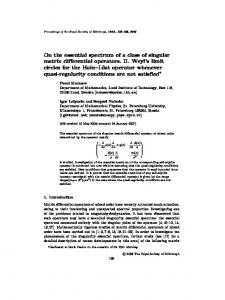
thus we have MY = λY, and we complete the proof. Example 3.1. Let G = (V, E) be the Petersen graph as Figure 1. Let {V1 , V2 } be a partition

of V = {1, 2, . . . , 10}, where V1 = {1, 2, 3, 4, 5} and V2 = {6, 7, 8, 9, 10}. Then the equi-

table quotient matrices B(A), B(L), B(Q), B(D), B(L), B(Q) corresponding to the adjacency

matrix A(G), the Laplacian matrix L(G), the signless Laplacian matrix Q(G), the distance matrix D(G), the distance Laplacian matrix L(G), the distance signless Laplacian matrix Q(G), respectively, are as follows:

1r

2

★❝ ★ ❝ ★ r6 ❝ ❝ ★ ✁ ❆ ❝ ★ ✁ ❆ 10 r r ❝r 5 ★ r 7❛ ✁ ❆ ✦ ❛❛ ✦✦ ❆ ✁ ✁ ❛ ❆ ❆ ✁ ✦✦❛❛ ❆r 9 ✁ ❆ 8 ✁r✦ ❆❆ ✁ ❆ ✁✁ ❆✁r ❆✁r

3 4 Figure 1. The Petersen graph

7



B(A) =  

B(D) = 

2 1 1 2

6 9 9 6



,



,



1

B(L) =  

B(L) = 

−1

−1

9 −9

1

−9 9



,



,



B(Q) =  

B(Q) = 

5 1 1 5



,

21

9

9

21



.

Then ρ(B(A)) = 3, ρ(B(L)) = 2, ρ(B(Q)) = 6, ρ(B(D)) = 15, ρ(B(L)) = 18, ρ(B(Q)) = 30, but by directly calculating, we have ρ(G) = 3, µ(G) = 5, q(G) = 6, ρD (G) = 15, µD (G)) = 18, q D (G) = 30. We see that the largest eigenvalue of the equitable quotient matrix B(M) is the largest eigenvalue of M when M is the adjacency matrix A(G), the signless Laplacian matrix Q(G), the distance matrix D(G), the distance Laplacian matrix L(G) or the distance signless Laplacian matrix Q(G) of a graph G, and the result is totally different when M is the Laplacian matrix L(G) of a graph G.

Lemma 3.3. Let M be defined as (3.1), and for any i, j ∈ {1, 2 . . . , t}, Mii = li Jni + pi Ini ,

Mij = sij Jni ,nj for i 6= j, where li , pi , sij are real numbers, B = B(M) be the quotient matrix of M. Then

[ni −1]

σ(M) = σ(B) ∪ {pi

| i = 1, 2 . . . , t},

(3.2)

where λ[t] means that λ is an eigenvalue with multiplicity t. Proof. It is obvious that for any i, j ∈ {1, 2 . . . , t}, Mij has constant row sum, so B is the

equitable quotient matrix of M. Then σ(B) ⊆ σ(M) by Lemma 3.2.

[ni −1]

On the other hand, we note that σ(li Jni + pi Ini ) = {li ni + pi , pi

}, where li Jni + pi Ini

has the all-one vector Jni ,1 such that (li Jni + pi Ini )Jni ,1 = (li ni + pi )Jni ,1 , and its all other eigenvectors corresponding to eigenvalue pi are orthogonal to Jni ,1 . Let x be an any eigenvector such that (li Jni + pi Ini )x = pi x, then xT Jni ,1 = 0, and (01,n1 , . . . , xT , . . . , 01,nt )T is an eigenvector of M corresponding to eigenvalue pi . Therefore the pi is an eigenvalue of M with multiplicities at least ni − 1. And thus we obtain at least Pt [n1 −1] [n −1] , . . . , pt t } ⊆ σ(M). i=1 (ni − 1) = n − t eigenvalues of M, that is, {p1 8

[n −1]

Therefore σ(B) ∪ {p1 1

[n −1]

|{p1 1

[nt −1]

, . . . , pt

[nt −1]

, . . . , pt

} ⊆ σ(M) by Lemma 3.2, and |σ(M)| ≤ |σ(B)| + [n −1]

}| = n by |σ(B)| = t and |{p1 1

[nt −1]

, . . . , pt

}| = n − t.

If there exists some pi such that pi ∈ σ(B) where i ∈ {1, 2, . . . , t}, by the proof of Lemma

3.2, we have My = pi y with y = (y11 , . . . , y1,n1 , . . . , yt1 , . . . , yt,nt )T , where yi1 = yi2 = . . . = yi,ni = yi for each i ∈ {1, 2, . . . , t}. Then we have (01,n1 , . . . , xT , . . . , 01,nt )y= yi (xT Jni ,1 ) = 0, it implies that the eigenvectors corresponding to the eigenvalue pi of B and the eigenvalue pi [n −1]

in {p1 1

[nt −1]

, . . . , pt

and thus (3.2) holds.

[n −1]

} are all orthogonal, then |σ(M)| = |σ(B)| + |{p1 1

[nt −1]

, . . . , pt

}| = n

Example 3.2. Let G = Kn1 ,n2 ,...,nt be a complete t-partite graph with n vertices for t ≥ 2, the

adjacency matrix A = A(G), the Laplacian matrix L = L(G), the signless Laplacian matrix Q = Q(G), the distance matrix D = D(G), the distance Laplacian matrix L = L(G) and the distance signless Laplacian matrix Q(G) of G = Kn1 ,n2 ,...,nt are as follows:

(1). A = M, where li = pi = 0, sij = 1 for i 6= j where i, j ∈ {1, 2, . . . , t}.

(2). L = M, where li = 0, pi = n − ni , sij = −1 for i 6= j where i, j ∈ {1, 2, . . . , t}. (3). Q = M, where li = 0, pi = n − ni , sij = 1 for i 6= j where i, j ∈ {1, 2, . . . , t}. (4). D = M, where li = 2, pi = −2, sij = 1 for i 6= j where i, j ∈ {1, 2, . . . , t}.

(5). L = M, where li = −2, pi = n + ni , sij = −1 for i 6= j where i, j ∈ {1, 2, . . . , t}.

(6). Q = M, where li = 2, pi = n + ni − 4, sij = 1 for i 6= j where i, j ∈ {1, 2, . . . , t}.

It is obvious that for any i, j ∈ {1, 2 . . . , t}, Mij has constant row sum. Then the corre-

sponding equitable quotient matrices are as follows:



   B(A) =   



   B(Q) =   

0 n1 .. .

n1

0 .. .

n1 n2

n − n1 n1 .. .

n2 · · · nt

n2

 · · · nt   , ..  .. . .   ··· 0

···

n − n2 · · · .. .. . . n2



nt nt .. .

· · · n − nt



n − n1

  −n 1  B(L) =  . ..   −n1





   B(D) =   

   ,  

9

−n2

···

−n2

· · · n − nt

n − n2 · · · .. .. . .

2n1 − 2 n1 .. . n1

n2

−nt

−nt .. .

···

2n2 − 2 · · · .. .. . . n2



   ,  

nt nt .. .

· · · 2nt − 2



   ,  



n − n1

  −n 1  B(L) =  . ..   −n1 

   B(Q) =   

n + 3n1 − 4



−n2

···

−nt

−n2

· · · n − nt

n − n2 · · · .. .. . .

−nt .. .

   ,  

···

n2

n + 3n2 − 4 · · · .. .. . .

n1 .. . n1



nt nt .. .

· · · n + 3nt − 4

n2

   .  

By Lemma 3.3, we have (1). PA (λ) = λn−t PB(A) (λ) = λn−t [

t Q

(λ + ni ) −

i=1

(2). PL (λ) =

t Q

t P

i=1

(λ − n + ni )ni −1 PB(L) (λ) = λ(λ − n)

(3). PQ (λ) =

i=1 t Q

=

t Q

t Q

ni

(λ + nj )].

j=1,j6=i t Q t−1

(λ − n + ni )ni −1 .

i=1

(λ − n + ni )ni −1 PB(Q) (λ)

i=1

(λ − n + ni )ni −1 [

i=1

t Q

(λ − n + 2ni ) −

i=1

(4). PD (λ) = (λ + 2)n−t PB(D) (λ) t t P Q ni = (λ + 2)n−t [ (λ − ni + 2) − i=1

i=1

(5). PL (λ) = (6). PQ (λ) = =

t Q

t Q

t P

ni

i=1

(λ − n − ni + 4)

i=1 t Q

ni −1

(λ − n − ni + 4)ni −1 [

i=1

(λ − n + 2nj )].

j=1,j6=i

(λ − nj + 2)]. ([17])

j=1,j6=i

(λ − n − ni )ni −1 PB(L) (λ) = λ(λ − n)t−1

i=1 t Q

t Q

t Q

i=1

(λ − n − ni )ni −1 .

PB(Q) (λ) t Q

(λ − n − 2ni + 4) −

i=1

t P

i=1

ni

t Q

(λ − n − 2nj + 4)].

j=1,j6=i

It is obvious that we obtain the spectrums of L and L immediately. In fact, σ(L) =

{0, n[t−1] , (n−ni )[ni−1] , i ∈ {1, 2, . . . , t}}, and σ(L) = {0, n[t−1] , (n+ni )[ni−1] , i ∈ {1, 2, . . . , t}}. A block of G is a maximal connected subgraph of G that has no cut-vertex. A graph G is a clique tree if each block of G is a clique. We call Ku,n2 ,...,nk+1 is a clique star if we replace each edge of the star K1,k by a clique Kni such that V (Kni ) ∩ V (Knj ) = u for i 6= j and

i, j ∈ {2, . . . , k + 1}.

Example 3.3. Let G = Ku,n2 ,...,nk+1 , where n1 = |{u}| = 1, ni ≥ 2 for any i ∈ {2, . . . , k + 1}

and n = n1 + n2 + n3 + . . . + nk+1 − k. Then the adjacency matrix A = A(G), the Laplacian matrix L = L(G), the signless Laplacian matrix Q = Q(G), the distance matrix D = D(G), 10

the distance Laplacian matrix L = L(G) and the distance signless Laplacian matrix Q(G) of

G = Ku,n2 ,...,nk+1 are as follows.

(1). A = M, where l1 = p1 = 0 and li = 1, pi = −1 for i 6= 1, sij = 1 for i = 1or j = 1,

and sij = 0 for any i, j ∈ {2, . . . , k + 1} and i 6= j.

(2). L = M, where l1 = n − 1, p1 = 0 and li = −1, pi = ni for i 6= 1, sij = −1 for

i = 1or j = 1, and sij = 0 for any i, j ∈ {2, . . . , k + 1} and i 6= j.

(3). Q = M, where l1 = n − 1, p1 = 0 and li = 1, pi = ni − 2 for i 6= 1, sij = 1 for

i = 1or j = 1, and sij = 0 for any i, j ∈ {2, . . . , k + 1} and i 6= j.

(4). D = M, where l1 = 0, p1 = 0 and li = 1, pi = −1 for i 6= 1, sij = 1 for i = 1or j = 1,

and sij = 2 for any i, j ∈ {2, . . . , k + 1} and i 6= j.

(5) L = M, where l1 = n − 1, p1 = 0 and li = −1, pi = 2n − ni for i 6= 1, sij = −1 for

i = 1or j = 1, and sij = −2 for any i, j ∈ {2, . . . , k + 1} and i 6= j.

(6). Q = M, where l1 = n − 1, p1 = 0 and li = 1, pi = 2n − ni − 2 for i 6= 1, sij = 1 for

i = 1or j = 1, and sij = 2 for any i, j ∈ {2, . . . , k + 1} and i 6= j.

It is obvious that for any i, j ∈ {2, . . . , k + 1}, Mij has constant row sum. Then the

corresponding equitable quotient matrices are as follows:



   B(A) =   



   B(Q) =   

0 n1 − 1 · · · nk − 1

1 n1 − 2 · · · .. .. .. . . . 1

n−1 1 .. .

1

0

0 .. .

· · · nk − 2

n1 − 1

···

2n1 − 3 · · · .. .. . . 0

nk − 1 0 .. .

n−1

  −1  B(L) =  .  ..  −1

n − 1 1 − n1

  −1  B(L) =  .  ..  −1

   ,  

· · · 2nk − 3 







   ,  

1 − n1



   B(D) =    ···

2n − 2n1 + 1 · · · .. .. . . −2(n1 − 1)

11

0

1 .. .

···

··· .. . . . .

1 − nk

0

···

1

   ,  

···

nk − 1

1 2n1 − 1 · · ·

nk − 2

1 .. .

n1 − 1

0 .. .



n1 − 2 .. .

1 − nk

−2(nk − 1) .. .

· · · 2n − 2nk + 1



   ,  

· · · 2nk − 1 .. .. . .



   ,  



n−1

   B(Q) =   

n1 − 1

1 .. .

···

nk − 1

2(n1 − 1) · · ·

2n − 3

2n − 3 .. .

1

· · · 2nk − 1 .. .. . .



   .  

By Lemma 3.3, we have (1). PA (λ) = (λ + 1)n−k−1PB(A) (λ) k+1 k+1 k+1 Q P Q = (λ + 1)n−k−1[λ (λ − ni + 2) − (ni − 1) (λ − nj + 2)]. i=2

i=2

j=2,j6=i

(2). PL (λ) = (λ − ni )ni −2 PB(L) (λ) = λ(λ − n)(λ − 1)k−1 (λ − ni )ni −2 . k+1 Q (3). PQ (λ) = (λ − ni + 2)ni −2 PB(Q) (λ) =

i=2 k+1 Q i=2

(λ − ni + 2)ni −2 [λ

k+1 Q i=2

(λ − 2ni + 3) −

k+1 P i=2

(ni − 1)

k+1 Q

(λ − 2nj + 3)].

j=2,j6=i

(4). PD (λ) = (λ + 1)n−k−1PB(D) (λ) k+1 k+1 k+1 Q P Q = (λ + 1)n−k−1[λ (λ + ni ) − (2λ + 1) (ni − 1) (λ + nj )]. i=2

i=2

j=2,j6=i

(5). PL (λ) = (λ − 2n + ni )ni −2 PB(L) (λ) = λ(λ − n)(λ − 2n + 1)k−1(λ − 2n + ni )ni −2 . k+1 Q (6). PQ (λ) = (λ − 2n + ni + 2)ni −2 PB(Q) (λ) =

i=2 k+1 Q i=2

(λ − 2n + ni + 2)ni −2 [(λ − n + 1)

−(2λ − 2n + 3)

k+1 P i=2

(ni − 1)

k+1 Q

k+1 Q i=2

(λ − 2n + 2ni + 1)

(λ − 2n + 2nj + 1)].

j=2,j6=i

It is obvious that we can obtain the spectrum of L and L immediately. In fact, σ(L) = [ni −2]

{0, n, 1[k−1], ni

{2, 3, . . . , k + 1}}.

, i ∈ {2, 3, . . . , k + 1}} and σ(L) = {0, n, (2n − 1)[k−1] , (2n − ni )[ni −2] , i ∈

By Lemma 3.2, Example 3.1 and Examples 3.2–3.3, we proposed the following conjecture for further research. Conjecture 3.4. Let M be a nonnegative matrix, B(M) be the equitable quotient matrix of M. Then the largest eigenvalue of B(M) is the largest eigenvalue of M. Consider two sequences of real numbers: λ1 ≥ λ2 ≥ ... ≥ λn , and µ1 ≥ µ2 ≥ ... ≥ µm with

m < n. The second sequence is said to interlace the first one whenever λi ≥ µi ≥ λn−m+i for

i = 1, 2, ..., m. The interlacing is called tight if there exists an integer k ∈ [1, m] such that

λi = µi hold for 1 ≤ i ≤ k and λn−m+i = µi hold for k + 1 ≤ i ≤ m.

Lemma 3.5. ([12]) Let M be a symmetric matrix and have the block form as (3.1), B be the quotient matrix of M. Then 12

(1) The eigenvalues of B interlace the eigenvalues of M. (2) If the interlacing is tight, then B is the equitable matrix of M. By Lemmas 3.2-3.5, we have the following result immediately. Theorem 3.1. Let M = (mij )n×n be a symmetric matrix and defined as (3.1), B = B(M) be the quotient matrix of M, and µ1 ≥ µ2 ≥ ... ≥ µm be all eigenvalues of B. Then µ1 , µ2, ..., µm are eigenvalues of M if and only if B is the equitable matrix of M.

4

Spectral radius of strongly connected digraphs with given connectivity

Let Ω(n, k) be the set of all simple strong connected digraphs on n vertices with vertex → − → − connectivity k. Let G 1 ▽ G 2 denote the digraph G = (V, E) obtained from two disjoint → − − → → − → − → − → − digraphs G 1 , G 2 with vertex set V = V ( G 1 ) ∪ V ( G 2 ) and arc set E = E( G 1 ) ∪ E( G 2 ) ∪ → − → − {(u, v), (v, u)|u ∈ V ( G 1 ), v ∈ V ( G 2 )}. → − Let p, k be integers with 1 ≤ k ≤ n − 2, 1 ≤ p ≤ n − k − 1, K (n, k, p) denote the − → − → − → − → → − digraph Kk ▽ (Kp ∪ K n−p−k ) ∪ E, where E = {(u, v)|u ∈ Kp , v ∈ K n−p−k }. Clearly, → − K (n, k, p) ∈ Ω(n, k). Then the adjacency matrix, the signless Laplacian matrix, the distance → − matrix, the distance signless Laplacian matrix of K (n, k, p) are as follows, where q = n−p−k. 

J p − Ip

 → − A( K (n, k, p)) =   Jk,p 

Jp + (n − 2)Ip

 → − Q( K (n, k, p)) =   Jk,p

Jk + (n − 2)Ik

J p − Ip

 → − D( K (n, k, p)) =   Jk,p

2Jq,p

Jp + (n − 2)Ip

2Jq,p

 Jk,q  , J q − Iq

Jq,k 

 → − Q( K (n, k, p)) =   Jk,p

J k − Ik

Jp,k

0q,p



Jp,q

Jq,k

0q,p



Jp,k



Jp,q

J k − Ik

 Jk,q  , J q − Iq

Jq,k

Jk + (n − 2)Ik Jq,k



 Jk,q  , Jq + (n − p − 2)Iq

Jp,k

Jp,k

13

Jp,q

Jp,q



 Jk,q  . Jq + (n + p − 2)Iq

→ − Proposition 4.1. ([2]) Let G be a strongly connected digraphs with vertex connectivity k. − → → − − → → − Suppose that S is a k-vertex cut of G and G 1 , G 2 , . . . , G t are the strongly connected com→ − → → − − → − ponents of G − S. Then there exists an ordering of G 1 , G 2 , . . . , G t such that for 1 ≤ i ≤ t i−1 S− → → − G j. and v ∈ V ( G i ), every tail of v is in j=1

→ − Remark 4.2. By Proposition 4.1, we know that G 1 is the strongly connected component → − → − → − → − − → of G − S where the inneighbors of vertices of V ( G 1 ) in G − S − G 1 are zero. Let G 2 = → − → − → − → − G − S − G 1 . We add arcs to G until both induced subdigraph of V ( G 1 ) ∪ S and induced → − → − subdigraph of V ( G 2 ) ∪ S attain to complete digraphs, add arc (u, v) for any u ∈ V ( G 1 ) and − → → − → − − → any v ∈ V (G2 ), the new digraph denoted by H . Clearly, H = K (n, k, p) ∈ Ω(n, k) for some → − → − p such that 1 ≤ p ≤ n − k − 1. Since G is the spanning subdigraph of H , then by Corollary → − → − → − → − → − → − 2.3, we have ρ( G ) ≤ ρ( K (n, k, p)), q( G ) ≤ q( K (n, k, p)), ρD ( G ) ≥ ρD ( K (n, k, p)) and → − → − q D ( G ) ≥ q D ( K (n, k, p)). Thus the extremal digraphs which achieve the maximal (signless Laplacian) spectral radius and the minimal distance (signless Laplacian) spectral radius in → − Ω(n, k) must be some K (n, k, p) for 1 ≤ p ≤ n − k − 1. → − Theorem 4.1. Let n, k be given positive integers with 1 ≤ k ≤ n − 2, G ∈ Ω(n, k). Then (i). ([20])

n−2+ − → ρ( G ) ≤

p

(4.1)

2n + k − 3 + − → q( G ) ≤

p

(4.2)

(n − 2)2 + 4k , 2 → − − → → − − → with equality if and only if G ∼ = K (n, k, 1) or G ∼ = K (n, k, n − k − 1). (ii). ([13])

(2n − k − 3)2 + 4k , 2

→ − − → with equality if and only if G ∼ = K (n, k, n − k − 1). (iii). ([22])

n−2+ − → ρD ( G ) ≥

p

(4.3)

3n − 3 + − → q (G) ≥

p

(4.4)

(n + 2)2 − 4k − 8 , 2 → − − → → − − → with equality if and only if G ∼ = K (n, k, 1) or G ∼ = K (n, k, n − k − 1). (iv).

D

(n + 3)2 − 8k − 16 , 2

→ − − → with equality if and only if G ∼ = K (n, k, 1). → − Proof. Now we show (i) holds. We apply Lemma 3.3 to A = A( K (n, k, p)). Since t = 3, li = 1, pi = −1 for 1 ≤ i ≤ 3, s31 = 0 and sij = 1 for others i, j ∈ {1, 2, 3} and i 6= j, we have σ(A) = σ(B(A)) ∪ {(−1)[n−3] }, where the corresponding equitable quotient matrix of A is 14



 B(A) =  

p−1 p 0

k

q

k−1

q

k

√



q−1

 ,  √

n−2+ 4p2 −4(n−k)p+n2 4p2 −4(n−k)p+n2 the eigenvalues of B(A) are −1, . Thus ρ(A) = . 2 2 √ √ 2 2 2 n−2+ (n−2) +4k n−2+ 4p −4(n−k)p+n ≤ , and equality holds if and only It is obvious that 2 2 n−2±

→ − − → if p = 1 or p = n − k − 1. Thus (4.1) holds and equality holds if and only if G ∼ = K (n, k, 1) → − − → or G ∼ = K (n, k, n − k − 1). → − Now we show (ii) holds. Similarly, we apply Lemma 3.3 to Q = Q( K (n, k, p)). Since t = 3, li = 1 for 1 ≤ i ≤ 3, p1 = p2 = n − 2, p3 = n − p − 2, s31 = 0 and sij = 1 for others

i, j ∈ {1, 2, 3} and i 6= j, we have σ(Q) = σ(B(Q)) ∪ {(n − 2)[p+k−2] , (n − p − 2)[q−1] }, where the corresponding equitable quotient matrix of Q is 

 B(Q) =  

p+n−2

the eigenvalues of B(Q) are n − 2,

p 0

k

q

k+n−2

q

k

(3n−p−4)±

√



q+n−p−2

(n−3p)2 +8pk . 2

 , 

Thus ρ(Q) =

3n−p−4+

√

(n−3p)2 +8pk . 2

By the same proof of Theorem 7.6 in [13], we can show (4.2) holds by proving 3n − p − 4 +

p

(n − 3p)2 + 8pk 2n + k − 3 + ≤ 2

p

(2n − k − 3)2 + 4k 2

→ − − → for 1 ≤ p ≤ n − k − 1, and equality holds if and only if G ∼ = K (n, k, n − k − 1). → − Now we show (iii) holds. We apply Lemma 3.3 to D = D( K (n, k, p)). Since li = 1, pi = −1 for 1 ≤ i ≤ 3, s31 = 2 and sij = 1 for others i, j ∈ {1, 2, 3} and i 6= j, we have σ(D) = σ(B(D)) ∪ {(−1)[n−3] }, and the corresponding equitable quotient matrix of D is 

 B(D) =  

p−1 p 2p

k

q

k−1

q

k

q−1



 , 

√ √ n−2+ −4p2 +4(n−k)p+n2 (n−2)± −4p2 +4(n−k)p+n2 . Thus ρ(D) = . the eigenvalues of B(D) are −1, 2 2 √ 2 √ 2 2 n−2+ (n+2) −4k−8 n−2+ −4p +4(n−k)p+n It is obvious that ≥ , and equality holds if and only 2 2 → → − − if p = 1 or p = n − k − 1. Thus (4.3) holds and equality holds if and only if G ∼ = K (n, k, 1) 15

→ − − → or G ∼ = K (n, k, n − k − 1).

→ − Now we show (iv) holds. We apply Lemma 3.3 to Q = Q( K (n, k, p)). Since l1 = l2 =

l3 = 1, p1 = p2 = n − 2, p3 = n + p − 2, s31 = 2 and sij = 1 for others i, j ∈ {1, 2, 3} and

i 6= j, we have σ(Q) = σ(B(Q)) ∪ {(n − 2)[p+k−2], (n + p − 2)[q−1] }, and the corresponding equitable quotient matrix of Q is 

 B(Q) =  

p+n−2 p 2p

the eigenvalues of B(Q) are n − 2, ρ(Q) =

Now we show

3n+p−4+

k

q

k+n−2

q

k

(3n+p−4)±

3n + p − 4 +

√

(n+3p)2 −16p2 −8kp 2

√

≥

q+n+p−2

(n+3p)2 −16p2 −8kp . 2

p



 , 

Thus

(n + 3p)2 − 16p2 − 8kp . 2

3n−3+

the equality holds if and only if p = 1. Let f (p) =

√

(n+3)2 −8k−16 for 1 ≤ p ≤ n − k 2 √ 3n+p−4+ (n+3p)2 −16p2 −8kp . Then 2

− 1, and

∂ 2 f (p) −4((2n − k)(n − k) + k 2 ) = 3 < 0. ∂p2 ((n + 3p)2 − 16p2 − 8kp) 2 Thus, for fixed n and k, the minimal value of f (p) must be taken at either p = 1 or p = n − k − 1. Let α = k 2 − 6k − 7 + 8n and β = n2 + 6n − 7 − 8k. Then 2[f (n − k − 1) − f (1)] = n − k − 2 +

√

α−

p

β = (n − k − 2)(1 − √

n+k √ ). α+ β

We can assume that n > k + 2 since in case k = n − 2 there is only one value of p under

consideration. Now suppose that f (n − k − 1) − f (1) ≤ 0. We will produce a contradiction.

We have

√

α+

p

p √ β ≤ n + k, α − β ≤ −n + k + 2.

√

α ≤ k + 1 and α ≤ (k + 1)2 which reduces to k ≥ n − 1 which of range. √ is out 2 −8k−16 → − → − (n+3) 3n−3+ Thus f (n − k − 1) > f (1) and q D ( G ) ≥ f (1) = q D ( K (n, k, 1)) = , with 2 →∼− − → equality if and only if G = K (n, k, 1). Whence

It is natural that whether there exists similar result for the Laplacian spectral radius or the distance Laplacian spectral radius in Ω(n, k) or not? In fact, we can obtain the spectrum

16

→ − of the Laplacian matrix or the distance Laplacian matrix of K (n, k, p) immediately. → − Proposition 4.3. Let K (n, k, p) defined as before. Then → − (i). σ(L( K (n, k, p))) = {0, n[p+k−1], (n − p)[q] }. → − (ii). σ(L( K (n, k, p))) = {0, n[p+k−1], (n + p)[q] }. → − − → Proof. Firstly, the Laplacian matrix L( K (n, k, p)) and the distance Laplacian matrix L( K (n, k, p)) → − of K (n, k, p) are the following matrices, where q = n − p − k. 

 → − L = L( K (n, k, p)) =   

 → − L = L( K (n, k, p)) =  

−Jp + nIp −Jk,p

−Jp,k

−Jk + nIk



−Jp,q

−Jk,q

 ,  

0q,p

−Jq,k

−Jq + (n − p)Iq

−Jp + nIp

−Jp,k

−Jp,q

−Jk,p

−2Jq,p

−Jk + nIk −Jq,k

−Jk,q

−Jq + (n + p)Iq

 . 

Then the corresponding equitable quotient matrices are as follows: 

n−p

 B(L) =   −p 0

−k

−q



 n − k −q  , −k k



n−p

 B(L) =   −p

−2p

−k

n−k −k

−q



 −q  . n+p−q

Then by Lemma 3.3 and directly calculating, we obtain (i) and (ii).

5

Spectral radius of connected graphs with given connectivity Let C(n, k) be the set of all simple connected graphs on n vertices with vertex connectivity

k. Let G1 ▽ G2 denote the graph G = (V, E) obtained from two disjoint graphs G1 , G2 by

joining each vertex of G1 to each vertex of G2 with vertex set V = V (G1 ) ∪ V (G2 ) and edge set E = E(G1 ) ∪ E(G2 ) ∪ {uv|u ∈ V (G1 ), v ∈ V (G2 )}.

Let p, k be integers with 1 ≤ k ≤ n − 2, 1 ≤ p ≤ n − k − 1, and K(n, k, p) be the graph

Kk ▽ (Kp ∪ Kn−p−k ). Clearly, K(n, k, p) ∈ C(n, k). Then the adjacency matrix, the signless

Laplacian matrix, the distance matrix, the distance signless Laplacian matrix of K(n, k, p) are as follows, where q = n − p − k. 17



J p − Ip

 A(K(n, k, p)) =   Jk,p 

J k − Ik

 Jk,q  , J q − Iq

Jq,k

Jp + (p + k − 2)Ip

Jp,k

0p,q

Jk + (n − 2)Ik Jq,k

0q,p



J p − Ip

 D(K(n, k, p)) =   Jk,p

2Jq,p



0p,q

0q,p

 Q(K(n, k, p)) =   Jk,p

Jp + (n + q − 2)Ip

 Q(K(n, k, p)) =   Jk,p

2Jq,p



Jp,k

J k − Ik Jq,k

 Jk,q  , Jq + (n − p − 2)Iq 2Jp,q

Jp,k



 Jk,q  , J q − Iq 2Jp,q

Jp,k Jk + (n − 2)Ik Jq,k





 Jk,q  . Jq + (n + p − 2)Iq

Remark 5.1. Let G be a connected graphs with vertex connectivity k. Suppose that S is a k-vertex cut of G, and G1 is a connected component of G − S. Let G2 = G − S − G1 , we add edges to G until both induced subgraph of V (G1 ) ∪ S and induced subgraph of V (G2 ) ∪ S

attain to complete graphs, the new graph denoted by H. Clearly, H = K(n, k, p) ∈ C(n, k)

for some p such that 1 ≤ p ≤ n − k − 1. Since G is the spanning subgraph of H, then by

Corollary 2.3, we have ρ(G) ≤ ρ(K(n, k, p)), q(G) ≤ q(K(n, k, p)), ρD (G) ≥ ρD (K(n, k, p))

and q D (G) ≥ q D (K(n, k, p)). Thus the extremal graphs which achieve the maximal (signless

Laplacian) spectral radius and the minimal distance (signless Laplacian) spectral radius in C(n, k) must be some K(n, k, p) for 1 ≤ p ≤ n − k − 1. Theorem 5.1. Let n, k be given positive integers with 1 ≤ k ≤ n − 2, G ∈ C(n, k). Then (i) ([28]) ρ(G) ≤ ρ(K(n, k, 1)), and ρ(K(n, k, 1) is the largest root of equation (5.1): λ3 − (n − 3)λ2 − (n + k − 2)λ + k(n − k − 2) = 0,

(5.1)

with equality holds if and only if G = K(n, k, 1). (ii) ([28]) q(G) ≤ q(K(n, k, 1)) =

2n + k − 4 + 18

p

(2n − k − 4)2 + 8k , 2

(5.2)

with equality holds if and only if G = K(n, k, 1). (iii) ([22]) ρD (G) ≥ ρD (K(n, k, 1)), and ρD (K(n, k, 1) is the largest root of equation (5.3): λ3 − (n − 3)λ2 − (5n − 3k − 6)λ + kn − k 2 + 2k − 4n + 4 = 0,

(5.3)

with equality holds if and only if G = K(n, k, 1). (iv) ([26]) q Q (G) ≥ q Q (K(n, k, 1)), and q Q (K(n, k, 1) is the largest root of equation (5.4): λ3 −(5n−k−6)λ2 +(8n2 −19kn−24n+8k+16)λ−4n3 +2(k+10)n2 −2(5k+16)n+12k+16 = 0, (5.4)

with equality holds if and only if G = K(n, k, 1). Proof. Firstly, we show (i) holds. We apply Lemma 3.3 to A = A(K(n, k, p)). Since t = 3, l1 = l2 = l3 = 1, p1 = p2 = p3 = −1, s13 = s31 = 0 and s12 = s21 = s23 = s32 = 1, we have

σ(A) = σ(B(A)) ∪ {(−1)[n−3] }, where the corresponding equitable quotient matrix of A is   p−1 k 0   B(A) =  k−1 q   p  , the eigenvalues of B(A) are the roots of the equation 0 k q−1 λ3 − (n − 3)λ2 + (pq − 2n + 3)λ + pq − n + pqk + 1 = 0.

(5.5)

It is obvious that ρ(A(K(n, k, p))) is the largest root of the equation (5.5). Now we show ρ(A(K(n, k, 1))) = max{ρ(A(K(n, k, p)))|1 ≤ p ≤ n − k − 1}. We note that

p + q = n − k and the adjacency matrix is symmetric, without loss of generality, we assume

that q ≥ p ≥ 1. Let fp,q (λ) = λ3 − (n − 3)λ2 + (pq − 2n + 3)λ + pq − n + pqk + 1. Let

H = Kk ▽ (Kp−1 ∪ Kq+1 ) = K(n, k, p − 1). Obviously, H ∈ C(n, k) and ρ(H) is the largest root of fp−1,q+1 (λ) = 0, then

fp,q (λ) − fp−1,q+1 (λ) = pqλ + pq + pqk − (p − 1)(q + 1)λ − (p − 1)(q + 1) − (p − 1)(q + 1)k and

= (q + 1 − p)(λ + k + 1) > 0,

fp,q (ρ(H)) = fp,q (ρ(H)) − fp−1,q+1(ρ(H)) > 0 = fp,q (ρ(K(n, k, p))).

It implies ρ(H) = ρ(K(n, k, p−1)) > ρ(K(n, k, p)). Thus ρ(G) ≤ ρ(K(n, k, 1)), ρ(K(n, k, 1))

is the largest root of the equation (5.1), ρ(G) = ρ(K(n, k, 1)) if and only if G = K(n, k, 1).

Second, we show (ii) holds. We apply Lemma 3.3 to Q = Q(K(n, k, p)). Since t = 3, l1 = l2 = l3 = 1, p1 = p + k − 2, p2 = n − 2, p3 = n − p − 2, s13 = s31 = 0 and s12 = s21 = 19

s23 = s32 = 1, we have σ(Q) = σ(B(Q)) ∪ {(p + k − 2)[p−1] , (n − 2)[k−1] , (n − p − 2)[q−1] } where the corresponding equitable quotient matrix of Q is 

 B(Q) =  

2p + k − 2 p 0

k

0

k+n−2

q



q+n−p−2

k

 , 

p the eigenvalues of B(Q) are n − 2, n − 2 + k2 ± 21 (k − 2n)2 + 16p(k − n + p). Thus ρ(Q) = p n − 2 + k2 + 21 (k − 2n)2 + 16p(k − n + p). p Let f (p) = n − 2 + k2 + 21 (k − 2n)2 + 16p(k − n + p), then f (1) = f (n − k − 1) = √ 2n+k−4+ (2n−k−4)2 +8k , and we complete the max{f (p)|1 ≤ p ≤ n − k − 1}. Therefore, q(G) ≤ 2 proof of (ii) by K(n, k, 1) ∼ = K(n, k, n − k − 1).

Third, we show (iii) holds. We apply Lemma 3.3 to D = D(K(n, k, p)). Since t = 3,

l1 = l2 = l3 = 1, p1 = p2 = p3 = −1, s13 = s31 = 2 and s12 = s21 = s23 = s32 = 1, we have σ(D) = σ(B(D)) ∪ {(−1)[n−3] } where the corresponding equitable quotient matrix of D is 

 B(D) =  

p−1 p 2p

k

2q

k−1

q

k

q−1



 , 

the eigenvalues of B(D) are the roots of the equation: λ3 − (n − 3)λ2 − (3pq + 2n − 3)λ + pqk − 3pq − n + 1 = 0.

(5.6)

It is obvious that ρ(D(K(n, k, p))) is the largest root of the equation (5.6). Similar to the proof of (i), we can show (iii) holds, we omit it. Finally, we show (iv) holds. We apply Lemma 3.3 to Q = Q(K(n, k, p)). Since t = 3,

l1 = l2 = l3 = 1, p1 = n + q − 2, p2 = n − 2, p3 = n + p − 2, s13 = s31 = 2 and s12 = s21 =

s23 = s32 = 1, we have σ(Q) = σ(B(Q)) ∪ {(n + q − 2)[p−1] , (n − 2)[k−1], (n + p − 2)[q−1]} where the corresponding equitable quotient matrix of Q is 

n+p+q−2

 B(Q) =   p

2p

k n+k−2 k

2q



 q  , n+p+q−2

the eigenvalues of B(Q) are the roots of the equation: λ3 − (5p + 5q + 4k − 6)λ2 + (8p2 + 8q 2 + 20

5k 2 + 12pq + 13pk + 13qk − 20p − 20q − 16k + 12)λ − 4p3 − 4q 3 − 2k 3 − 8p2 q − 8pq 2 − 10p2 k −

10q 2k −8pk 2 −8qk 2 −16pqk +16p2 +16q 2 +10k 2 +24pq +26pk +26qk −20p−20q −16k +8 = 0. Similar to the proof of (i), we can show (iv) holds, we omit it.

It is natural that whether there exists similar result for the Laplacian spectral radius or the distance Laplacian spectral radius in C(n, k) or not? In fact, we can obtain the spectrum of the Laplacian matrix or the distance Laplacian matrix of K(n, k, p) immediately. Proposition 5.2. Let K(n, k, p) defined as before. Then (i). σ(L(K(n, k, p))) = {0, k, n[k], (p + k)[p−1] , (q + k)[q−1] }.

(ii). σ(L(K(n, k, p))) = {0, n + p + q, n[k] , (n + q)p−1, (n + p)q−1 }.

Proof. Firstly, the Laplacian matrix L(K(n, k, p)) and the distance Laplacian matrix L(K(n, k, p))

of K(n, k, p) are the following matrices, where q = n − p − k. 

 L = L(K(n, k, p)) =   

 L = L(K(n, k, p)) =  

−Jp + (p + k)Ip −Jk,p

−Jp,k

−Jk + nIk



0p,q −Jk,q

 ,  

0q,p

−Jq,k

−Jq + (q + k)Iq

−Jp + (n + q)Ip

−Jp,k

−2Jp,q

−Jq,k

−Jq + (n + p)Iq

−Jk,p

−2Jq,p

−Jk + nIk

−Jk,q

 . 

Then the corresponding equitable quotient matrices are as follows: 

k

−k

0



  , B(L) =  −p n − k −q   0 −k k



 B(L) =  

n+q−p −p

−2p

−k

−2q

−k

n+p−q

n−k

−q



 . 

Then by Lemma 3.3 and directly calculating, we obtain (i) and (ii).

References [1] M. Aouchiche, P. Hansen, Two Laplacian for the distance matrix of a graph, Linear Algebra Appl. 439 (2013) 21–33. [2] J.A. Bondy, U.S.R. Murty, Graph Theory with Applications, Macmillan, London, 1976. 21

[3] Abraham Berman, Robert J. Plemmons, Nonnegative Matrices in the Mathematical Sciences, New York: Academic Press, 1979. [4] R. Brualdi, Spectra of digraphs, Linear Algebra Appl. 432 (2010) 2181–2213. [5] Andries E. Brouwer, Willem H. Haemers, Spectra of graphs - Monograph -, Springer, 2011. [6] S. Burcu Bozkurt and Durmus Bozkurt, On the signless Laplacian spectral radius of digraphs, Ars Combinatoria, 108 (2013) 193–200. [7] D. Cvetkovic, P. Rowlinson, S. Simic, An Introduction to the Theory of Graph Spectra, London, 2010. [8] Y.Y. Chen, H.Q. Lin, J.L. Shu, Sharp upper bounds on the distance spectral radius of a graph, Linear Algebra Appl. 439 (2013) 2659–2666. [9] S.W. Drury, H.Q. Lin, Extremal digraphs with given clique number, Linear Algebra Appl. 439 (2013) 328–345. [10] Roman Drnovsˆek, The spread of the spectrum of a nonnegative matrix with a zero diagonal element, Linear Algebra Appl. 439 (2013) 2381–2387. [11] X. Duan, B. Zhou, Sharp bounds on the spectral radius of a nonnegative matrix, Linear Algebra Appl. 439 (2013) 2961–2970. [12] W.H. Haemers, Interlacing eigenvalues and graph, Linear Algebra Appl. 226–228 (1995) 593–616. [13] W.X. Hong, L.H. You, Spectral radius and signless Laplacian spectral radius of strongly connected digraphs, Linear Algebra Appl. 457 (2014) 93–113. [14] R.A. Horn, Charles R. Johnson, Matrix Analysis, Cambridge University Press, 1986. [15] G. Indulal, I. Gutman, On the distance spectra of some graphs, Mathematical Communications, 13 (2008) 123–131. [16] J.B. Jensen, G. Gutin, Digraphs Theory, Algorithms and Applications, Springer, 2001. [17] H.Q. Lin, Y. Hong, J.F. Wang, J.L. Shu, On the distance spectrum of graphs, Linear Algebra Appl. 439 (2013) 1662–1669. 22

[18] H.Q. Lin, S.W. Drury, The maximum Perron roots of digraphs with some given parameters, Discrete Math. 313 (2013) 2607–2613. [19] H.Q. Lin, R.F. Liu, X.W. Lu, The inertia and energy of the distance matrix of a connected graph, Linear Algebra Appl. 467 (2015) 29–39. [20] H.Q. Lin, J.L. Shu, Y.R. Wu, G.L. Yu, Spectral radius of strongly connected digraphs, Discrete Math. 312 (2012) 3663–3669. [21] H.Q. Lin, J.L. Shu, The distance spectral radius of digraphs, Discrete Applied Math. 161 (2013) 2537–2543. [22] H.Q. Lin, W.H. Yang, H.L. Zhang, J.L. Shu, Distance spectral radius of digraphs with given connectivity, Discrete Math. 312 (2012) 1849–1856. [23] Chia-an Liu, Chih-wen Weng, Spectral radius of bipartite graphs, arXiv:1402.5621v1 [math.CO] 23 Feb 2014. [24] Z.Z. Liu, On spectral radius of the distance matrix, Appl. Anal. Discrete Math. 4 (2010) 269–277. [25] O. Rojo, E. Lenes, A sharp upper bound on the incidence energy of graphs in terms of connectivity, Linear Algebra Appl. 438 (2013) 1485–1493. [26] R. Xing, B. Zhou and J. Li, On the distance signless Laplacian spectral radius of graphs, Linear and Multilinear Algebra, 62 (2014) 1377–1387. [27] M.L. Ye, Y.Z. Fan, D. Liang, The least eigevalue of graphs with given connectivity, Linear Algebra Appl. 430 (2009) 1375–1379. [28] M.L. Ye, Y.Z. Fan, H.F. Wang, Maximizing signless Laplacian or adjacency spctral radius of graphs subject to fixed connectivity, Linear Algebra Appl. 433 (2010) 1180–1186. [29] X.L. Zhang, The inertia and energy of the distance matrix of complete k-partite graphs, Linear Algebra Appl. 450 (2014) 108–120.

23