Spectrum Sensing Performance in TV Bands using the Multitaper Method Tugba Erpek† , Alexe Leu∗ , and Brian L. Mark† † Dept.
of Electrical and Comp. Eng. George Mason University 4400 University Drive, MS 1G5 Fairfax, VA 22030, U.S.A. { terpek, bmark }@gmu.edu
Abstract— Frequency agile radios perform opportunistic spectrum sharing by detecting unused spectrum and dynamically tuning to the available bands. To reduce harmful interference to the primary users of the spectrum, highly sensitive detectors are required. We apply the multitaper spectral estimation method to the problem of spectrum sensing in TV bands. We compare the performance of the multitaper method with that of conventional FFT-based spectrum estimation, using real signal measurements. Our results show that the multitaper approach yields a significant increase in the number of harvested channels, while maintaining a smaller probability of false alarm. ¨ ¸e – Ozetc Frekans-atik radyolar kullanılmayan frekans kus¸aklarını saptayıp dinamik olarak o kanalda iletime gec¸erek frekans izge paylas¸ımına olanak sa˘glarlar. Paylas¸ım ile frekans kanalındaki birincil kullanıcıların iletimini etkilememek icin ¨ duyarlılı˘gı yuksek dedekt¨orlere ihtiyac¸ vardır. Bu c¸alıs¸mada, ¨ gerc¸ek sinyal o¨ lc¸umleri kullanılarak c¸oklu pencereleme y¨ontemi ¨ ¸ yo˘gunlu˘gu elde edilmis¸tir. Elde ile TV bantlarında izgel guc edilen sonuc¸lar, periodogram y¨ontemi sonunda elde edilen ¨ ¸ yo˘gunlu˘gu ile kars¸ılas¸tırılmıs¸tır ve c¸oklu pencereleme izgel guc ¨ ¸uk ¨ kaldı˘gı y¨ontemi kullanıldı˘gında, yanlıs¸ alarm olasılı˘gı dus halde frekans paylas¸ımı ile kullanılabilecek kanal sayısında artıs¸ oldu˘gu g¨ozlenmis¸tir.
I. I NTRODUCTION Recent studies of wireless spectrum usage [1], [2] have shown that a large portion of the spectrum is highly underutilized. Such studies suggest that significant gain in wireless capacity could be achieved by means of opportunistic spectrum sharing. To realize this gain, a method of accurately identifying spectrum holes is needed. A spectrum hole can be defined as frequency band that is not being used by a primary user at a particular time and geographic region [3]. Spectrum sharing could be performed by frequency agile radios (FARs), which have the capability of dynamically tuning to spectrum holes within a frequency range. To determine the spectrum holes accurately, a FAR node should be equipped with a highly sensitive detector and an algorithm to access the unused spectrum without causing harmful interference to the primary users of the spectrum. The Listen-Before-Talk (LBT) scheme [4], is a simple method for
∗ Shared
Spectrum Company 1595 Spring Hill Road Vienna, VA 22182, U.S.A.
[email protected]
a FAR node to access unused spectrum opportunistically. For LBT to be effective, the sensitivity of the detector is required to be about 30 to 50 dB below the TV receiver sensitivity. Detecting signals below the thermal noise level is very important for spectrum sharing in TV bands, because higher detector sensitivity enables higher transmit power levels. Spectrum holes are determined by examining the power spectral density of the received signal. Therefore, accurate and efficient methods of power spectral estimation are important for determining the spectrum hole accurately. In this paper, we compare the spectrum harvesting performance of conventional FFT-based spectral estimation with the multitaper (MT) method [5], applied to TV signal measurements. Section II describes the two spectral estimation methods used in this paper for spectrum hole detection: the MT method and the FFT method. Section III describes the measurement site and the empirical data used to obtain the performance curves presented in Section IV. Conclusions are given in Section V. II. S PECTRAL E STIMATION In [4], ultra-sensitive TV detector measurements are analyzed using the conventional FFT-based method. The MT method was introduced by Thomson [5] and has been shown to have superior performance in some applications such as geoclimate sensing [6]. Haykin [7] suggests that the multitaper method would be effective in spectrum sharing applications, but we are not aware of empirical studies applying the multitaper method to spectrum hole detection using real measurement data. In [4], the conventional FFT method is used to study TV detector measurement data. In the present paper, we compare the performance of the FFT method versus the MT method with respect to spectrum sensing using the empirical TV measurement data from [4]. A. Conventional FFT Method Given a time series, {X1 ,X2 ,. . . ,XN }, the conventional FFT method estimates the power spectral density S(·) as follows: 2 N ∆t X −j2πf t∆t fft Xt e (1) S (f ) , , N t=1
where ∆t is the spacing between the samples. The function S fft (f ) is known as the periodogram [8]. The periodogram is an unbiased estimate of the power spectral density for white Gaussian noise, but its variance is equal to a constant that is independent of the data length N . As a result, Var[S fft (f )] 6= 0 as N → ∞.
III. S IGNAL M EASUREMENT DATA
Hence, the periodogram is an inconsistent estimator of the power spectrum [8]. B. Multitaper Method Multitaper spectral analysis is a method for spectral estimation of a time series that is believed to exhibit a spectrum containing both continuous and singular components. This method involves the use of a set of K orthogonal tapers, called Discrete Prolate Spheroidal Sequence (DPSS) tapers. K represents the tradeoff between resolution and the variance properties of the spectral estimate. The variance of the spectral estimate can be decreased when K is large. On the other hand, we smear out the fine features and decrease the resolution of the spectral estimate by increasing the value of K. The kth taper is a sequence {ht,k : t = 0, 1, · · · , N }. Each taper provides protection against spectral leakage [5]. The time series data is windowed with each of the K DPSS tapers and then a periodogram is computed via the FFT [9]. The high resolution multitaper spectrum is a weighted sum of K eigenspectra, Sˆkmt (·), k = 0, · · · , K − 1 (see [8], p. 369): K−1 X
S mt (f ) ,
λk Sˆkmt (f )
k=0 K−1 X
,
(2)
λk
k=0
where
2 N X mt −j2πf t∆t ˆ Sk (f ) , ∆t ht,k Xt e , t=1
ht,k is the tth DPSS taper element for the kth direct spectral estimator Sˆkmt (·), and λk is the eigenvalue corresponding to the eigenvector with elements {ht,k } (see [8], p. 103). A more leakage-resistant spectral estimate, called an adaptively weighted multitaper (AWMT) spectrum, can be obtained by adjusting the relative weights on the contributions from each of the K eigenspectra as follows (see [8], p. 370): K−1 X
S amt (f ) ,
(3) b2k (f )λk
k=0
where bk (f ) is a weighting function that further guards against broadband leakage for a non-white (“colored”) but locally-white process. The weight of the kth eigenspectrum is proportional to b2k (f )λk , where S(f ) . bk (f ) = λk S(f ) + (1 − λk )σ 2 ∆t
The signal measurement data used in this paper is taken from [10]. The TV signals are in the NTSC signal format and data from TV channels 2 – 10 are used in this paper. The carrier signal for channel 2 is located at a frequency of 55.25 MHz and the channel spacing is 6 MHz. The power of the carrier signal contributes about 25% of the total signal power in a channel. Spectrum measurements were made at a residential location in McLean, Virginia. The equipment was connected to a standard TV antenna located on the second story roof. The measurement data consists of time series data collected over a period of approximately 8 minutes for 40 different starting times. Thus, we have a collection of M = 40 sets of time (i) series data available to us, which we represent by {Xt }, (i) where Xt denotes the tth sample in the ith data set with i = 1, · · · , M and t = 1, · · · , N , where N = 819, 200. The time spacing between samples is ∆t = 0.586 ms. IV. N UMERICAL R ESULTS Figs. 1 and 2 show three types of graphs corresponding to the FFT and MT methods, respectively: a) maximum hold (max-hold) plot, b) waterfall plot, and c) duty cycle plot. We applied both the standard MT and the AWMT methods to the data and observed no significant difference in the results. The results presented in this paper are obtained using AWMT method with K = 7 tapers. Let Si (f ) denote the spectral estimate obtained from the first N = 18, 000 samples of the ith data set or time series (using the FFT method or the MT method). The max-hold power spectral estimate is defined by Smh (f ) , max Si (f ), fl ≤ f ≤ fh , 1≤i≤M
(4)
where fl = 61.2 MHz and fh = 61.3 MHz. The waterfall plot shows the set of points (f, i), for which the spectral estimate Si (f ) exceeds a given threshold η over the M data sets. The set of points in the waterfall plot can be expressed as W , {(f, i) : Si (f ) ≥ η, 1 ≤ i ≤ M, fl ≤ f ≤ fh }.
b2k (f )λk Sˆkmt (f )
k=0 K−1 X
Parseval’s theorem is satisfied in expected value in (2), because the weights in the estimator do not depend on the frequency. On the other hand, the AWMT spectral estimator given in (3) generally does not satisfy Parseval’s theorem in expected value [8].
(5)
The duty cycle plot shows, for each frequency f , the proportion of data sets for which Si (f ) exceeds the threshold η. In other words, the value of the duty cycle plot at the frequency value f is given by d(f ) ,
M 1 X 1{Si (f )≥η} , fl ≤ f ≤ fh , M i=1
(6)
where 1A denotes the indicator function on the set A. Thus, the duty cycle plot renders negligible spectral components that have high power for only a small number of data sets.
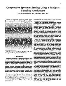
Number of correctly identified busy channels vs. threshold level 5 4.5
61.21
61.22
61.23
61.24 61.25 61.26 Frequency (MHz)
61.27
61.28
61.29
Data set
40 20 0
61.21
61.22
61.23
61.24 61.25 61.26 Frequency(MHz)
61.27
61.28
61.29
Duty Cycle
1
Correctly Identified Busy Channels
Max Hold (dBm)
McLean TV Channel 3 FFT frequency resolution =5.0Hz -80 -100 -120 -140 -160 -180
4 3.5 3 2.5 2 1.5 1
0.5 0.5 0
Fig. 1.
61.21
61.22
61.23
61.24 61.25 61.26 Frequency in MHz
61.27
61.28
61.29
Max-hold plot for TV channel 3 using the FFT method.
0 -120
Fig. 3.
FFT(1500 samples) MT(1500 samples) -100
-80 -60 -40 Detector threshold level (dBm)
-20
0
Number of correctly identified busy channels vs. threshold value.
Max Hold (dBm)
McLean TV Channel 3 MT frequency resolution =5.0Hz -80 -100 -120 -140 -160 -180
61.21
61.22
61.23
61.24 61.25 61.26 Frequency (MHz)
61.27
61.28
61.29
61.21
61.22
61.23
61.24 61.25 61.26 Frequency(MHz)
61.27
61.28
61.29
61.21
61.22
61.23
61.24 61.25 61.26 Frequency in MHz
61.27
61.28
61.29
Data set
40 20
Duty Cycle
0
Fig. 2.
1 0.5 0
Max-hold plot for TV channel 3 using the MT method.
For the waterfall and duty cycle plots in Figs. 1 and 2, detector threshold values of η = −110 dBm and η = −119 dBm were used, respectively. Comparing these two figures, we can make the following qualitative observations. From the maxhold plots, we see a smaller variation in the spectral estimates obtained via the MT method. The average signal level in the max-hold plot is lower in the case of the MT method, since it is able to suppress more of the noise components. From the waterfall plots, we see that the MT method removes misleading information. From the duty cycle plots obtained using the MT method, we can much more easily identify the carrier signal and the synchronization pulses, which are 15 kHz apart from each other in each channel. The duty cycle plots can be used to determine whether a channel is free or occupied at a specific time. The performance curves shown in Figs. 3-6 were obtained using duty cycle plots for which the detector threshold value η was varied from −120 to 0 dBm. To obtain these figures, power spectrum estimates corresponding to each of the M = 40 data sets were computed using the first N = 1500 samples from each
set. Note that this number of samples corresponds to a time period of approximately 35 seconds. Then duty cycle values are computed using (6) for a given value of η. Fig. 3 shows the number of correctly identified busy channels versus the threshold level for both the FFT method and the MT method. A channel is identified as busy (i.e., a signal is present) if the duty cycle value d(f ) corresponding to the carrier frequency exceeds a threshold of 0.2 (i.e., 20%). In the MT method, the noise components of the signal and the variance of the spectral estimate are reduced such that the power of the MT-based estimate is less than that of the FFT-based estimate. As a result, the number of detected channels is higher for the FFT method when the threshold level is between -70 dB and -30 dB. However, in practice, such high values would not be used as a detector threshold; opportunistic spectrum access requires much lower detector thresholds. The objective here is to decrease the threshold as much as possible in order to obtain accurate information about spectrum occupancy. Fig. 4 shows the number of false alarm channels versus the detector threshold level. A false alarm channel refers to a channel that is identified as busy, when it is actually free. We observe that the number of false alarm channels is lower for the MT method when the threshold level is between -120 and -80 dBm. Fig. 5 shows the number of miss-detected channels versus the detector threshold. A miss-detected channel refers to a channel that is identified as free, when it is actually busy. The number of miss-detected channels is the same for both MT and FFT methods for the threshold levels of interest. Fig. 6 shows the number of correctly identified free channels versus the detector threshold. The correctly identified free channels represent the channels that are available for spectrum sharing. The number of correctly identified free channels is higher with MT method between −120 and −80 dBm. If we set a fixed threshold level, e.g. -100 dB and examine the statistics using this threshold level, we can see that the number of correctly identified busy channels and the number of missdetected channels are the same for both methods. On the other
hand, the number of false alarm channels is lower and the number of correctly identified free channels is higher for the MT method. Thus, we see that more channels can be harvested by means of the MT method compared with the FFT method, using a lower threshold level.
Number of false alarm channels vs. threshold level 4 FFT(1500 samples) MT(1500 samples)
3.5
False Alarm Channels
3 2.5
V. C ONCLUSION
2 1.5 1 0.5 0 -120
Fig. 4.
-100
-80 -60 -40 Detector threshold level (dBm)
-20
0
Number of false alarm channels vs. threshold value.
Number of miss detected channels vs. threshold level 5 4.5
FFT(1500 samples) MT(1500 samples)
Miss Detected Channels
4 3.5 3 2.5
In this paper, we applied the multitaper (MT) method of spectral estimation to the problem of spectrum harvesting in TV bands. The computational complexity of the MT method is greater than that of the FFT method by a factor of K, where K is the number of tapers used. However, for relatively small time series, e.g., 1500 samples taken over 40 different data sets amounts to about 35 seconds, the MT method is fast enough to be used in real-time. We compared the performance spectrum harvesting using the conventional FFT method versus the MT method using empirical TV measurement data. From the max-hold, waterfall, and duty cycle plots, we can observe, qualitatively, the noise reduction properties of the MT method relative to the FFT method. Our preliminary results with TV measurement data indicate that the noise reduction property of the MT method can result in a significant gain in the number of correctly identified free channels compared to the FFT method. This suggests that significant gains in spectrum harvesting may be achievable in more general settings. In ongoing work, we are applying the MT method to larger sets of measurement data from a variety of signal sources.
2
ACKNOWLEDGMENT
1.5 1 0.5 0 -120
-100
-80 -60 -40 Detector threshold level (dBm)
-20
0
The authors would like to thank Dr. Kathleen Wage for helpful discussions on the multitaper method. This work was supported in part by the U.S. National Science Foundation under Grant No. CCR-0209049 and Grant No. ECS-0426925. R EFERENCES
Fig. 5.
Number of miss-detected channels vs. threshold value.
Number of correctly identified free channels vs. threshold level 4
Correctly Identified Free Channels
3.5 3 2.5 2 1.5 1 0.5 0 -120
Fig. 6.
FFT(1500 samples) MT(1500 samples) -100
-80 -60 -40 Detector threshold level (dBm)
-20
0
Number of correctly identified free channels vs. threshold value.
[1] M. McHenry, “Frequency agile spectrum access technologies,” in Proc. FCC Workshop on Cognitive Radio, May 2003. [2] G. Staple and K. Werbach, “The end of spectrum scarcity,” IEEE Spectrum, vol. 41, pp. 48–52, March 2004. [3] P. Kolodzy, “Next generation communications: Kickoff meeting,” in Proc. DARPA, October 2001. [4] A. E. Leu, M. McHenry, and B. L. Mark, “Modeling and analysis of interference in listen-before-talk spectrum access schemes,” Int. J. Network Mgmt, vol. 16, pp. 131–147, 2006. [5] D. J. Thomson, “Spectrum Estimation and Harmonic Analysis,” Proc. IEEE, vol. 70, pp. 1055–1096, September 1982. [6] M. E. Mann and J. Park, “Oscillatory spatiotemporal signal detection in climate studies: A multiple-taper spectral domain approach,” Advances in Geophysics, vol. 41, pp. 1–131, 1999. [7] S. Haykin, “Cognitive Radio: Brain-Empowered Wireless Communications,” IEEE J. Selected Areas in Comm., vol. 23, pp. 201–220, Feb. 2005. [8] D. B. Percival and A. T. Walden, Spectral Analysis for Physical Applications. Cambridge University Press, 1993. [9] T. P. Bronez, “On the Performance Advantage of Multitaper Spectral Analysis,” IEEE Trans. on Signal Proc., vol. 40, pp. 2941–2946, December 1992. [10] A. E. Leu, K. Steadman, M. McHenry, and J. Bates, “Ultra Sensitive TV Detector Measurements,” in Proc. IEEE Int. Symp. on New Frontiers in Dynamic Spectrum Access Networks (DySPAN), pp. 30–36, Nov. 2005.