Speech Detection in the Noisy Environment Using Wavelet Transform Juraj Kačur1, Juraj Frank2, Gregor Rozinaj3 1
Department of Telecommunications, FEI STU, Ilkovičová 3, Bratislava, Slovakia, e-mail:
[email protected], phone: +421-2- 68279416 2 Department of Telecommunications, FEI STU Ilkovičová 3, Bratislava, Slovakia, e-mail:
[email protected] 3 Department of Telecommunications, FEI STU, Ilkovičová 3, Bratislava, Slovakia, e-mail:
[email protected], phone: +421-2- 68279414
Abstract In this article we present speech detection systems based on Daubechie, Coiflet and Symlet wavelet transforms respectively. For each a selection of the most eligible levels of signal decomposition for the corrupted speech detection problem was made. Using those levels the distinction between noise and corrupted signal can be amplified as far as 100 times. Tests were accomplished using a set of Slovak words artificially noised to several SNR by white WSS noise. Key words: speech detection, WSS noises, Wavelet transforms, multi-resolution analysis.
1 Introduction The task of voice activity detection consists of labelling speech end-points in audio signals. Speech contains high-energy vowels of various lengths as well as unvoiced consonants of low energy and higher frequency components, all varied in the time (even intervals of silence can be part of speech). Added noises can dramatically deteriorate the whole detection process, because they can dispose of various characteristics that makes their separation from speech sometime almost impossible. Driving motivations behind this article are the application areas like: speech compression and transmission, speech recognition, etc. and the promising results of DWT employment in signal processing.
2 Wavelet transform Classical Fourier transform works well in wide sense stationary signals, but is of little use in non-stationary signals, because of its hidden localization information. This was amended by the short time FT, which on the other hand leads to the spectral distortion due to the window properties [1]. Still, by STFT we can achieve only uniform time- frequency distribution and harmonic basis functions. Many of wavelet transforms can eliminate these weaknesses. Their main advantages that are crucial in our development follow:
• • • •
They provide explicit localization of events in the signal that is very true if scaling and wavelet function have compact support. Various time-frequencies distribution can be achieved (logarithmic most usual). Theoretically there is an unlimited number of scaling and wavelet functions. DTW can be easily realized by filter bank or lifting scheme [4].
Using Wavelet transforms any signal or function belonging to L2 can be expressed by (1): ∞
g (t ) = ∑ ci ( k )ϕ i ,k (t ) + ∑∑ d j ( k )ψ j ,k (t ) (1) k
k
j =i
Where φk(t) and ψjk(t) are scaling and wavelet functions respectively. The expansion coefficients c(k) and dj(k) can be calculated as the inner product of a signal and wavelet or scaling functions. Scaling function and all its integral shifts form the basis of the coarsest sub space V0 of L2. The rest of L2 is then covered by infinite set of disjunctive spaces (W0, W1, …) each of which is represented by the integral time shifts of a given wavelet function, i.e. L2= V∞=V0 ∪ W0 ∪ W1 ∪ W2 ∪… Space V1=V0∪W0 is determined by the basis functions of V0 being time shifted and time scaled versions (shrunk by factor 2). Then scaling and wavelet functions of V0 can be expressed by (2) in the terms of V1 basis functions: ϕ (t ) = ∑ h (n ) 2ϕ (2t − n ) ,
ψ (t ) = ∑ h1 (n ) 2ϕ ( 2t − n ) (2)
n
n
Both functions are derived as a linear combination of scaling functions from V1. Where h(n) and h1(n) are weights of the length N and they form low pass and high pass FIR filters respectively. Then expansion coefficients cj(k) and dj(k) in different levels of decomposition can be calculated using (3). c j ( k ) = ∑ h ( m − k ) c j +1 ( m ) , m
d j ( k ) = ∑ h1 ( m − k ) c j +1 ( m )
(3)
m
Equations (3) are called the analysis part of the DWT and their synthesis counterparts are given in (4): c j +1(k ) = ∑c j (m)h(k − 2m) + ∑d j (m)h1 (k − 2m) (4) m
m
Those formulas were derived for continuous signals. In the discrete case, signal samples are regarded as coefficients cj(k) in the uppermost level. This is a good approximation for most wavelet systems as their wavelet functions at those levels act as the Dirac function when the calculation of their inner products with tested signal is performed. There are many necessary and sufficient conditions that a wavelet system must meet. For example a 2-band orthogonal wavelet system must fulfil following simultaneous equations (5):
∑ h ( k ) h ( k + 2 m ) = δ ( m ), n
N
∑ h(n) = n =1
2,
∑ h(k )h
1
( k + 2 m ) = 0 (5 )
n
Where δ(m) is the Kroneker unit impulse and N is the length of low pass filter. Other conditions and properties can be found e.g. in [2]. Chosen wavelets i.e. Daubechies, Coiflets and Symlets are well-known, orthonormal systems with following features. In Daubechie systems the freedom given by (5) is used to set to zero all moments of the mother wavelet spanning W0 up to k-th order (6).
m1 ( k ) = ∫ t kψ 0 (t ) dt = 0 (6)
This maximizes the smoothness of both scaling and wavelet functions (important for expansion of smooth signals). Coiflet systems have both moments of scaling and wavelet functions set to zero up to some order where the length of h(n) is kept minimal. This provides better approximation of the expansion coefficients by the samples of signal and produces more symmetric scaling functions too. Symmetry is the pursued property of Symlet wavelets (they are not completely symmetric) derived from the class of Daubachie wavelets. Other systems can use this freedom to meet different properties.
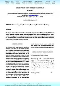
Figure 1. Scaling and wavelet functions generated by Daubechie system with the filter length 12 samples.
3 Speech detection based on wavelets In the first stage of the detection algorithm a signal is processed in order that the distinction between noise and sections of signal is amplified by proper transformation. Second stage measures and evaluates those features and takes the final decision. Both parts are equally important and related and thus chronologically explained in the following. As speech signals are well characterized by their frequency, energy and time structure it is sensible to require the transform to be orthogonal. This along with the compact support basis ensures the true energy localisation in the time as well as provides satisfactory frequency distribution, vital for analysis of non- stationary signals. Furthermore, taking into account human sound perception, audio signal analysis should be done in the similar way to the logarithmic band division [3], referring to concepts like: critical bands, Mel frequency spectrum, etc. Those requirements usually significantly constrain the freedom the designers may demand, but we can liberate the strict condition on full reconstruction, which is pointless for speech analysis. Finally, employment of wavelets is straightforward and can be even faster than FFT using the lifting scheme [4]. Keeping up to the abovementioned facts we decided for two-band (logarithmic frequency tilling) orthogonal systems. We deliberated to test and to compare the usage of basic wavelet classes in this area of speech processing. The basic idea is that smooth wavelet or scaling functions at certain levels (Wi,..Wj) should take up the most information from voiced parts of speech when broad-band noise is assumed. On the contrary unvoiced consonant and broadband noises with zero mean strongly tend to be expressed by high-resolution levels. The task is to find those resolution levels and proper wavelet functions, which do it best. Certain insight into this
can be made by observing courses of wavelet and scaling functions, e.g. fig.1. The more the course resembles the course of voiced speech the better distinction can be obtain. In the second stage a threshold-based decision-taking algorithm is employed. It tests the values of expansion coefficients at W5 level that proved to be well distinctive against a threshold set up during the design process. The threshold was set to minimize the miss ratio. Then a fine adjustment of both boundaries is performed at more detailed level (W12) shifting them closer to each other till additional thresholds are met. This operation is not needed but it can further decrease the mean detection error at the expense of higher miss ratio. This simple and fast magnitude checking algorithm is in place due to the orthogonality principle and the fact that a good approximation of voiced speech can be achieved by eligible wavelet functions at certain levels in contrary to broadband noise.
Figure 2 Detection errors as a function of the length of FIR filters for Cioflet, Symlet and Daubechie systems.
4. Experiments and results All tests were executed at the special set of 36 Slovak words. Each word was located in separate wav file (8kHz, 16 bits) with intervals of silence before and after the utterance. Those words were artificially noised by white noise in following SNR: 0, 3, 7, 10, 13 and 17dB. We accomplished experiments with Daubechie, Coiflet and Symlet DWT. Each can produce different shapes of wavelet and scaling functions according to the length of FIR filters. In fig. 2 the mean detection errors are depicted as a function of the filter length. This provided us with the proper range of filters lengths for each class. Others very important parameters to be found are the most significant resolution levels for speech detection affected by broadband noises. This is best viewed by the ratio of averaged absolute coefficients (intensity) in the corrupted speech to the average absolute values of those coefficients taken from noise only. Those ratios are shown in fig. 3 for all SNR and meaningful resolution levels in case of Symlet -17. For comparison reasons we present in fig. 4 these ratios measured in “raw” signal so that the significant separation of noise by applied DWT can be highlighted. Finally, fig. 5 depicts the mean detection error as a function of SNR for all tested wavelet classes.
Figure 3 Ratios of mean absolutes values in the Figure 4 Ratios of mean intensities of noised words to noise only parts distributed over some words to noise only parts as a function of SNR resolution levels as a function of SNR. It is the Symlet wavelet system of the FIR length 17
5. Conclusions • As fig. 5 shows the detection error is not a declining function of SNR as it may have been expected. This can be well explained as follows. First, some parameters, which can not be adjusted in the process of detection or it would made the system too complicated, were set up for the case of SNR 10 dB, which may not be the optimal for other values. Second, the presences of speech artefacts outside utterances (expiration, lip clicking) are more eminent at higher values of SNR. Finally, it is a proof of good separation of voiced parts by the wavelet systems in broadband noise at these SNR. Further degradation related to low SNR occurs in Figure 5. The mean detection errors in milliseconds for Daubechies, Coiflets and more adverse environment than tested. Symlets as a function of SNR • From fig. 4 it can be inferred that short filters may not provide best results which can be caused by poor frequency separation into bands or that wavelet functions are not smooth enough to copy voiced speech segments because they miss enough zeros to do so. In contrary, long filters would fall short in the fine time localization. The proper range is from 30 to 60, but it depends on the wavelet system. • Too coarse or detailed levels of resolution do not reflect voiced sounds which carry most energy of the speech signals and thus are easily detected even in low SNR. Eligible intervals can be determined following figure 3. It can be seen that intensity ratios of those coefficients in
noised signals and noises can reach up to 250, where 100 is a common value. In the contrary, without DWT analysis part these ratios are within the range from 1 to 10 (fig. 4). That shows a substantial improvement in speech / noise distinction, based on the intensity measure. • Originally we aimed to detect transient events in the speech by the means of DWT. This approach turned out to be of little use in speech signals since those are not as significant and obvious as in image processing where this approach can be used for edge detection [2]. Additional noises with sharp courses would make this task almost impossible. • Although these methods are restricted to broad-band noises, they present flexible systems which can be tailored to suite the given environment. It is still possible to utilize the knowledge of the environment to create optimal wavelet functions “on line” so that the distinction between noise and speech is kept high; however this would be much more difficult and many other problems would have to be solved. Other improvements can be reached by even more flexible time frequency distribution like that given by e.g. Wavelet pockets, Multi-wavelets.
References [1] G. Rozinaj, J. Polec, J. Kotuliaková, P. Podhradský, A. Marček, S. Merchevský a kolektív : Číslicové spracovanie signálov II, FABER Bratislava, 1997 [2] C. S. Burrus, R. A. Gopinath, H. Guo, Introduction to Wavelets and Wavelet Transforms a Primer, Prentice Hall, New Jersey, 1998 [3] L. Rabiner, Biing-Hwang Juan: Fundamentals of speech recognition, Prentice Hall PTR, 1993 [4] R. Vargic, PhD Thesis: Kompresia statického obrazu s využitím waveletovej transformácie a lifting schémy, Bratislava, 1999