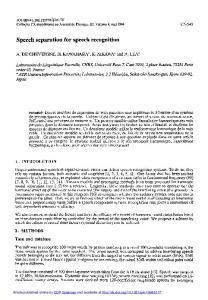
Nov 8, 2010 - Speech Recognition with Segmental Conditional Random Fields: Final ..... The recently released SCARF toolkit [2] is designed to support ...
Speech Recognition with Segmental Conditional Random Fields: Final Report from the 2010 JHU Summer Workshop Geoffrey Zweig1 Patrick Nguyen1 Dirk Van Compernolle2 Kris Demuynck2 Les Atlas3 Pascal Clark3 Greg Sell4 Fei Sha5 Meihong Wang5 Aren Jansen6 7 7 7 Hynek Hermansky Damianos Karakos Keith Kintzley Samuel Thomas7 Sivaram GSVS7 Sam Bowman8 Justine Kao4 November 8, 2010
1
Microsoft Research Leuven University 3 University of Washington 4 Stanford University 5 University of Southern California 6 JHU HLT COE 7 Johns Hopkins University 8 University of Chicago 2
Contents Acknowledgements
4
1 Workshop Goal
5
2 The 2.1 2.2 2.3 2.4
. . . . . . . . . . . . . . . . .
. . . . . . . . . . . . . . . . .
. . . . . . . . . . . . . . . . .
. . . . . . . . . . . . . . . . .
. . . . . . . . . . . . . . . . .
. . . . . . . . . . . . . . . . .
. . . . . . . . . . . . . . . . .
. . . . . . . . . . . . . . . . .
. . . . . . . . . . . . . . . . .
. . . . . . . . . . . . . . . . .
. . . . . . . . . . . . . . . . .
. . . . . . . . . . . . . . . . .
. . . . . . . . . . . . . . . . .
. . . . . . . . . . . . . . . . .
. . . . . . . . . . . . . . . . .
. . . . . . . . . . . . . . . . .
. . . . . . . . . . . . . . . . .
. . . . . . . . . . . . . . . . .
. . . . . . . . . . . . . . . . .
. . . . . . . . . . . . . . . . .
. . . . . . . . . . . . . . . . .
. . . . . . . . . . . . . . . . .
. . . . . . . . . . . . . . . . .
. . . . . . . . . . . . . . . . .
. . . . . . . . . . . . . . . . .
. . . . . . . . . . . . . . . . .
. . . . . . . . . . . . . . . . .
. . . . . . . . . . . . . . . . .
. . . . . . . . . . . . . . . . .
. . . . . . . . . . . . . . . . .
. . . . . . . . . . . . . . . . .
. . . . . . . . . . . . . . . . .
. . . . . . . . . . . . . . . . .
. . . . . . . . . . . . . . . . .
. . . . . . . . . . . . . . . . .
6 6 7 9 10 10 11 12 12 12 12 12 13 13 13 14 14 15
. . . . . . .
. . . . . . .
. . . . . . .
. . . . . . .
. . . . . . .
. . . . . . .
. . . . . . .
. . . . . . .
. . . . . . .
. . . . . . .
. . . . . . .
. . . . . . .
. . . . . . .
. . . . . . .
. . . . . . .
. . . . . . .
. . . . . . .
. . . . . . .
. . . . . . .
. . . . . . .
. . . . . . .
. . . . . . .
. . . . . . .
. . . . . . .
. . . . . . .
. . . . . . .
. . . . . . .
. . . . . . .
. . . . . . .
. . . . . . .
. . . . . . .
. . . . . . .
. . . . . . .
. . . . . . .
. . . . . . .
. . . . . . .
16 16 17 18 19 19 20 22
4 Data Sets and Baselines 4.1 Broadcast News . . . . . . . . . . . . . . 4.1.1 BN Database . . . . . . . . . . . 4.1.2 Baseline System . . . . . . . . . 4.1.3 Multi Phone Units . . . . . . . . 4.1.4 Processing the Data for SCARF 4.1.5 MSR Word Detectors . . . . . . 4.1.6 Some Standard Comparisons . . 4.2 Wall Street Journal . . . . . . . . . . . . 4.2.1 WSJ Database . . . . . . . . . . 4.2.2 HMM Baseline . . . . . . . . . .
. . . . . . . . . .
. . . . . . . . . .
. . . . . . . . . .
. . . . . . . . . .
. . . . . . . . . .
. . . . . . . . . .
. . . . . . . . . .
. . . . . . . . . .
. . . . . . . . . .
. . . . . . . . . .
. . . . . . . . . .
. . . . . . . . . .
. . . . . . . . . .
. . . . . . . . . .
. . . . . . . . . .
. . . . . . . . . .
. . . . . . . . . .
. . . . . . . . . .
. . . . . . . . . .
. . . . . . . . . .
. . . . . . . . . .
. . . . . . . . . .
. . . . . . . . . .
. . . . . . . . . .
. . . . . . . . . .
. . . . . . . . . .
. . . . . . . . . .
. . . . . . . . . .
. . . . . . . . . .
. . . . . . . . . .
. . . . . . . . . .
. . . . . . . . . .
. . . . . . . . . .
. . . . . . . . . .
. . . . . . . . . .
23 23 23 23 24 25 26 26 27 27 27
2.5
2.6
SCARF Framework Overview . . . . . . . . . . . . . . . . . Model . . . . . . . . . . . . . . . . . . . Adapting SCRFs for Speech Recognition Computation with SCRFs . . . . . . . . 2.4.1 Forward Backward Recursions . 2.4.2 Gradient Computation . . . . . . 2.4.3 Decoding . . . . . . . . . . . . . Features . . . . . . . . . . . . . . . . . . 2.5.1 Nomenclature . . . . . . . . . . . 2.5.2 Detector Inputs . . . . . . . . . . 2.5.3 Existence Features . . . . . . . . 2.5.4 Expectation Features . . . . . . . 2.5.5 Levenshtein Features . . . . . . . 2.5.6 Language Model Features . . . . 2.5.7 Baseline Features . . . . . . . . . 2.5.8 External Features . . . . . . . . Related Work . . . . . . . . . . . . . . .
3 SCARF Extensions 3.1 Computing with SCRFs . . . . . . . 3.2 Empirical Bayes Risk . . . . . . . . . 3.2.1 Forward-backward algorithm 3.2.2 Edge-based risk . . . . . . . . 3.3 Mixture Models . . . . . . . . . . . . 3.3.1 Sentence mixture models . . 3.3.2 Word-level mixtures . . . . .
. . . . . . .
1
4.2.3 4.2.4
DTW Baseline . . . . . . . . . . . . . . . . . . . . . . . . . . . . . . . . . . . . . . . . . . . . . 27 Processing the data for SCARF . . . . . . . . . . . . . . . . . . . . . . . . . . . . . . . . . . . 28
5 Template Features 5.1 Improving the Template-DTW Baseline System . . 5.1.1 Motivation . . . . . . . . . . . . . . . . . . . 5.1.2 Weighted k-NN Scores . . . . . . . . . . . . 5.1.3 Local Sensitivity Matrix . . . . . . . . . . . . 5.1.4 DTW Scoring . . . . . . . . . . . . . . . . . . 5.1.5 Word Based Templates . . . . . . . . . . . . 5.2 Extracting Template Features for use with SCARF 5.2.1 Motivation . . . . . . . . . . . . . . . . . . . 5.2.2 Approach . . . . . . . . . . . . . . . . . . . . 5.2.3 Template Based Meta-features . . . . . . . . 5.2.4 Optimization and Integration in SCARF . . .
. . . . . . . . . . .
. . . . . . . . . . .
. . . . . . . . . . .
. . . . . . . . . . .
. . . . . . . . . . .
. . . . . . . . . . .
. . . . . . . . . . .
. . . . . . . . . . .
. . . . . . . . . . .
. . . . . . . . . . .
. . . . . . . . . . .
. . . . . . . . . . .
. . . . . . . . . . .
. . . . . . . . . . .
. . . . . . . . . . .
. . . . . . . . . . .
. . . . . . . . . . .
. . . . . . . . . . .
. . . . . . . . . . .
. . . . . . . . . . .
. . . . . . . . . . .
. . . . . . . . . . .
. . . . . . . . . . .
. . . . . . . . . . .
. . . . . . . . . . .
30 30 30 30 31 31 33 33 33 33 34 35
6 MLP Neural Net Phoneme Detectors 6.1 Background . . . . . . . . . . . . . . . . . . . . . . . . . . . 6.2 Building Phoneme Detectors . . . . . . . . . . . . . . . . . 6.2.1 Hierarchical estimation of posteriors . . . . . . . . . 6.3 Integrating Detectors with SCARF . . . . . . . . . . . . . . 6.4 Experiments . . . . . . . . . . . . . . . . . . . . . . . . . . . 6.4.1 Oracle experiments to verify use of detectors . . . . 6.4.2 Usefulness of individual phoneme detectors . . . . . 6.4.3 Combining phoneme detectors with a word detector 6.4.4 When do phoneme detectors help the most? . . . . . 6.5 Summary . . . . . . . . . . . . . . . . . . . . . . . . . . . .
. . . . . . . . . .
. . . . . . . . . .
. . . . . . . . . .
. . . . . . . . . .
. . . . . . . . . .
. . . . . . . . . .
. . . . . . . . . .
. . . . . . . . . .
. . . . . . . . . .
. . . . . . . . . .
. . . . . . . . . .
. . . . . . . . . .
. . . . . . . . . .
. . . . . . . . . .
. . . . . . . . . .
. . . . . . . . . .
. . . . . . . . . .
. . . . . . . . . .
. . . . . . . . . .
. . . . . . . . . .
. . . . . . . . . .
. . . . . . . . . .
. . . . . . . . . .
. . . . . . . . . .
36 36 36 37 38 38 38 39 39 40 41
7 Deep Net Phoneme Detectors 7.1 Background . . . . . . . . . . . . . . . . . . 7.2 Deep Architectures . . . . . . . . . . . . . . 7.3 Deep Architecture for Phoneme Recognition 7.3.1 Unsupervised learning of RBM . . . 7.3.2 Stacking RBMs . . . . . . . . . . . . 7.3.3 Supervised learning of RBMs . . . . 7.3.4 Phoneme Recognition . . . . . . . . 7.4 Experiment Setup . . . . . . . . . . . . . . 7.5 Results . . . . . . . . . . . . . . . . . . . . . 7.6 Other work . . . . . . . . . . . . . . . . . .
. . . . . . . . . .
. . . . . . . . . .
. . . . . . . . . .
. . . . . . . . . .
. . . . . . . . . .
. . . . . . . . . .
. . . . . . . . . .
. . . . . . . . . .
. . . . . . . . . .
. . . . . . . . . .
. . . . . . . . . .
. . . . . . . . . .
. . . . . . . . . .
. . . . . . . . . .
. . . . . . . . . .
. . . . . . . . . .
. . . . . . . . . .
. . . . . . . . . .
. . . . . . . . . .
. . . . . . . . . .
. . . . . . . . . .
. . . . . . . . . .
. . . . . . . . . .
. . . . . . . . . .
. . . . . . . . . .
. . . . . . . . . .
. . . . . . . . . .
. . . . . . . . . .
. . . . . . . . . .
. . . . . . . . . .
. . . . . . . . . .
. . . . . . . . . .
. . . . . . . . . .
42 42 42 43 43 43 44 44 44 45 45
8 Point Process Model 8.1 Background . . . . . . . . . . . . . . . . . 8.2 Model Architecture . . . . . . . . . . . . . 8.2.1 Phone Event-Based Representation 8.2.2 Point Process Models . . . . . . . 8.3 PPM-Based Multiphone Unit Detection . 8.4 PPM-Based Word Lattice Annotations . . 8.5 Summary . . . . . . . . . . . . . . . . . .
. . . . . . .
. . . . . . .
. . . . . . .
. . . . . . .
. . . . . . .
. . . . . . .
. . . . . . .
. . . . . . .
. . . . . . .
. . . . . . .
. . . . . . .
. . . . . . .
. . . . . . .
. . . . . . .
. . . . . . .
. . . . . . .
. . . . . . .
. . . . . . .
. . . . . . .
. . . . . . .
. . . . . . .
. . . . . . .
. . . . . . .
. . . . . . .
. . . . . . .
. . . . . . .
. . . . . . .
. . . . . . .
. . . . . . .
. . . . . . .
. . . . . . .
. . . . . . .
. . . . . . .
46 46 46 47 47 50 51 53
9 Modulation Features 9.1 Background . . . . . . . . . . . . . . . . . . . . . . . . . . . . . . . . . . . . . . 9.2 Speech Features Based on a Bandwidth-Constrained Modulation Signal Model 9.3 Demodulation Methods . . . . . . . . . . . . . . . . . . . . . . . . . . . . . . . 9.3.1 Convex Demodulation . . . . . . . . . . . . . . . . . . . . . . . . . . . . 9.3.2 Pitch-Invariant Coherent Demodulation . . . . . . . . . . . . . . . . . .
. . . . .
. . . . .
. . . . .
. . . . .
. . . . .
. . . . .
. . . . .
. . . . .
. . . . .
. . . . .
. . . . .
. . . . .
. . . . .
54 54 54 56 56 57
. . . . . . .
2
. . . . . . . . . . .
. . . . . . . . . . .
. . . . . . . . . . .
9.4 9.5 9.6
9.3.3 Hilbert Envelope Demodulation . . . . . . . . . . Multiphone Discrimination with Modulation Templates Modulation Lattice Annotation for SCRF-Based ASR . Conclusion . . . . . . . . . . . . . . . . . . . . . . . . .
10 Duration Models 10.1 Background . . . . . . . . . . . . . 10.2 Discriminative Duration Modeling 10.2.1 Duration distributions . . . 10.2.2 Prepausal lengthening . . . 10.2.3 Word span confusions . . . 10.2.4 Designing duration features 10.3 Integrated Experiments . . . . . . 10.4 Discussion . . . . . . . . . . . . . .
. . . . . . . .
. . . . . . . .
. . . . . . . .
. . . . . . . .
. . . . . . . .
11 Cohort-Based Word Detectors 11.1 Cohort Sets . . . . . . . . . . . . . . . . . . 11.2 Cohort Set Generation and Statistics . . . . 11.3 Creating and Using Cohort-Based Detectors 11.4 Results . . . . . . . . . . . . . . . . . . . . . 12 Integrated Results 12.1 Broadcast News . . . . . . . . . . . . . . . 12.2 Wall Street Journal . . . . . . . . . . . . . 12.2.1 Improved DTW System . . . . . 12.2.2 Template Based System with Meta 12.2.3 System Combination with HMMs
. . . . . . . .
. . . . . . . .
. . . . for . .
. . . .
. . . .
. . . .
. . . .
. . . .
. . . .
. . . .
. . . .
. . . .
. . . .
. . . .
. . . .
. . . .
. . . .
. . . .
. . . .
. . . .
. . . .
. . . .
. . . .
. . . .
. . . .
. . . .
. . . .
. . . .
. . . .
58 58 60 61
. . . . . . . .
. . . . . . . .
. . . . . . . .
. . . . . . . .
. . . . . . . .
. . . . . . . .
. . . . . . . .
. . . . . . . .
. . . . . . . .
. . . . . . . .
. . . . . . . .
. . . . . . . .
. . . . . . . .
. . . . . . . .
. . . . . . . .
. . . . . . . .
. . . . . . . .
. . . . . . . .
. . . . . . . .
. . . . . . . .
. . . . . . . .
. . . . . . . .
. . . . . . . .
. . . . . . . .
. . . . . . . .
. . . . . . . .
62 62 62 62 63 64 65 65 66
. . . . . . . . . . . . . . . . . . . . . . . . Lattice Annotation . . . . . . . . . . . . .
. . . .
. . . .
. . . .
. . . .
. . . .
. . . .
. . . .
. . . .
. . . .
. . . .
. . . .
. . . .
. . . .
. . . .
. . . .
. . . .
. . . .
. . . .
. . . .
67 67 68 68 69
. . . . .
. . . . .
. . . . .
. . . . .
. . . . .
. . . . .
. . . . .
. . . . .
. . . . .
. . . . .
. . . . .
. . . . .
. . . . .
. . . . .
. . . . .
. . . . .
. . . . .
. . . . .
. . . . .
70 70 70 70 72 72
. . . . . . . .
. . . . . . . .
. . . . . . . .
. . . . . . . .
. . . . . . . . . . . . . . . . . . . . . Information . . . . . . .
13 Conclusion
. . . . . . . .
. . . . .
. . . . .
. . . . .
. . . . .
. . . . .
. . . . .
. . . . .
. . . . .
74
3
Acknowledgements We thank NSF grant IIS-0833652 for supporting the workshop, with supplemental funding from Google Research, Microsoft, and the JHU HLT Center of Excellence. F.S. and M.W. were furthur supported by NSF and DARPA grant and contract numbers NSF 0957742 and DARPA N10AP20019. F.S. and M.W. further thank Abdel-rahman Mohamed (U. of Toronto) for sharing his codes and expertise in training deep learning architecture. S.T. was funded by the Office of the Director of National Intelligence (ODNI), Intelligence Advanced Research Projects Activity (IARPA), through the Army Research Laboratory (ARL). D.V.C and K.D. were supported by FWO travel grant K.2.105.10N, FWO research grant G.0260.07, and the EU MC-RT Network “Sound-to-Sense.” L.A. thanks AFOSR grant FA9550-09-1-0060. We would like to thank the IBM Corporation for the use of the Attila Speech Recognizer to build state-of-the-art baseline systems. We would in particular like to acknowledge Brian Kingsbury for his invaluable assistance with the Broadcast News setup and in running Attila.
4
Chapter 1
Workshop Goal Novel techniques in speech recognition are often hampered by the long road that must be followed to turn them into fully functional systems capable of competing with the state-of-the-art. In the 2010 JHU summer workshop, we explored the use of Segmental Conditional Random Fields as an integrating technology to augment the best conventional systems with information from novel scientific approaches. The Segmental CRF approach [1] is a modeling technique in which the probability of a word sequence w is estimated from some observed features o as P (w|o) using a log-linear model. Described in Sec. 2.2, the model determines the probability of a word sequence by weighting features which each measure some form of consistency between a hypothesis and the underlying audio. These features are at the word-segment level, and for example a feature might be the similarity between observed and expected formant tracks. To ensure that the performance of a baseline system can be achieved, a built-in binary feature tests whether a hypothesized word is the same as that present at the same time in some baseline output. The key characteristic of the SCRF approach is that it provides a principled yet flexible way to integrate multiple information sources: all feature weights are learned jointly, using the conditional maximum likelihood (CML) objective function. In particular, SCRFs can combine information • of different types, for example both real valued and binary features; • at different granularities, for example at the frame, phoneme or word level • of varying quality, for example from a state-of-the-art baseline and from less accurate phoneme or word detectors • of varying degrees of completeness, for example a feature that detects just one word • that may be redundant, for example from phoneme and syllable detectors This flexibility is hard to achieve in standard systems, and opens new possibilities for the integration of novel information sources. The recently released SCARF toolkit [2] is designed to support research in this area, and was used at the workshop. Over the course of the workshop we exploited several information sources to improve performance on Broadcast News and Wall Street Journal tasks, including: • Template features [3] • Neural-net phoneme detectors, both MLP based [4, 5] and with Restricted Boltzman Machine pretraining [6] • Word detectors based on Point Process Models [7] • Modulation feature [8, 9] based multiphone detectors • Duration models In the remainder of the report, we first summarize the SCRF model, then describe these information sources and their results in isolation, and finally present experimental results combining multiple information sources.
5
Chapter 2
The SCARF Framework 2.1
Overview
SCARF is a toolkit for using Segmental Conditional Random Fields (SCRFs) to do speech recognition. The inspiration for SCARF comes from Maximum Entropy (ME) models, in which one may use thousands of possibly redundant features in a model to do classification. However, whereas ME models are best suited to “flat” n-way classification tasks, SCRFs are naturally suited to sequence labeling problems in which a sequence of labels (words) is assigned to an arbitrarily long input sequence. In this respect, SCRFs draw from earlier Conditional Random Field (CRF) models, which were designed for sequence labeling. SCRFs extend these models by operating at the segment level, in which multiple adjacent observations can be lumped together into a segment with a single label, and segment-level features can be extracted and used. In essence, SCRFs can be thought of as combining the sequence labeling properties of CRFs with the segment labeling properties of ME models. These properties are illustrated in Table 2.1. The use of SCRFs in speech recognition has several potential advantages: • As with Maximum Entropy models, they offer a convenient way to combine numerous, possibly redundant features. Unlike feature vectors as used in HMMs, we do not need to worry about keeping the features uncorrelated. • Since the analysis is done at the segment level, long-span features such as pitch contours can be extracted and related directly to the word hypothesis for a segment. • The models are inherently discriminative in nature. Unlike HMM models, in which discriminative training methods such as MMI, MPE and MCE are applied in a separate “add-on” process, discriminative training is built into SCRFs. In addition to the general advantages of SCRFs mentioned above, the SCARF implementation in particular has several important points which are worth mentioning: • N-gram language modeling has been fully incorporated, and one can easily choose whether to use a pre-trained maximum likelihood model, or to learn its parameters discriminatively, in an integrated fashion with the acoustic model parameters. • SCARF takes as its basic input acoustic detector events (see, e.g., [10, 11]. These may be, for example, phoneme detections or syllable detections. A wide variety of features can be automatically generated from these basic inputs. • SCARF has been designed to facilitate some of the operations that are commonly done with speech recognizers based on generative models. For example, the language model and lexicon can be changed without retraining. • The segmental computations are made efficient through the use of lattice constraints. When derived from an existing HMM system, this can be a convenient way to build on the state-of-the-art.
6
Framewise Analysis Segmental Analysis
Generative Model HMM Segmental HMM
Discriminative Model CRF SCRF
Table 2.1: Classification of model types along two dimensions. • SCARF supports user-defined features in the form of lattice annotations. This makes is simple to test the effect of new features without modifying any code.
2.2
Model
Figure 2.1: Graphical representation of a CRF. Segmental Conditional Random Fields - also known as Semi-Markov Random Fields [12] or SCRFs - form the theoretical underpinning for SCARF. They relax the Markov assumption from the frame level to the word level, where states now correspond with a variable and automatically derived time span. To explain these, we begin with the standard Conditional Random Field model [13], as illustrated in Figure 2.1. Associated with each vertical edge v are one or more feature functions fk (sv , ov ) relating the state variable to the associated observation. Associated with each horizontal edge e are one or more feature functions gd (sel , ser ) defined on adjacent left and right states. (We use sel and ser to denote the left and right states associated with an edge e.) The set of functions (indexed by k and d) is fixed across segments. A set of trainable parameters λk and ρd are also present in the model. The conditional probability of the state sequence s given the observations o is given by P P exp( v,k λk fk (sv , ov ) + e,d ρd gd (sel , ser )) P P P (s|o) = P ′e ′e ′ e,d ρd gd (sl , sr )) v,k λk fk (sv , ov ) + s′ exp(
In speech recognition applications, the labels of interest, words, span multiple observation vectors, and the exact labeling of each observation is unknown. Hidden CRFs [14] address this issue by summing over all labelings consistent with a known or hypothesized word sequence. However, in the recursions presented in [14], the Markov property is applied at the frame level, with the result that segmental properties are not modeled. The C-Aug model [15, 16] is also related, in applying a conditonal model at the segmental level, with a particular set of features derived from the Fisher kernel. Here, in order to use long-span features, and to directly relate segment-level acoustic properties to the word label, we adopt the formalism of segmental CRFs. In contrast to a CRF, the structure of the model is not fixed a priori. Instead, with N observations, all possible state chains of length l ≤ N are considered, with the observations segmented into l chunks in all possible ways. Figure 2.2 illustrates this. The top part of this figure shows seven observations broken into three segments, while the bottom part shows the same observations partitioned into two segments. For a given segmentation, feature functions are defined as with standard CRFs. Because of the segmental nature of the model, transitions only occur at logical points, and it is clear what span of observations to use to model a given symbol. Since the g functions already involve pairs of states, it is no more computationally expensive to expand the f functions to include pairs of states as well, as illustrated in Figure 2.3. This structure has the further benefit of allowing us to drop the distinction between g and f functions. To denote a block of original observations, we will use oji to refer to observations i through j inclusive. 7
Figure 2.2: A Segmental CRF and two different segmentations. In the semi-CRF work of [12], the segmentation of the training data is known. However, in speech recognition applications, this is not the case. Therefore, in computing sequence likelihood, we must consider all segmentations consistent with the state (word) sequence s, i.e. for which the number of segments equals the length of the state sequence. Denote by q a segmentation of the observation sequences, for example that of Fig. 2.3 where |q| = 3. The segmentation induces a set of (horizontal) edges between the states, referred to below as e ∈ q. One such edge is labeled e in Fig. 2.3. Further, for any given edge e, let o(e) be the segment associated with the right-hand state ser , as illustrated in Fig. 2.3. The segment o(e) will span a block of observations from some start time to some end time, 4 oet st ; in Fig, 2.3, o(e) is identical to the block o3 . (The first block of observations is handled by an implicit transition from a special start state to the first word.) With this notation, we represent all functions as fk (sel , ser , o(e)) where o(e) are the observations associated with the segment of the right-hand state of the edge. The conditional probability of a state (word) sequence s given an observation sequence o for a SCRF is then given by
P
q s.t. |q|=|s|
P (s|o) = P P
exp(
q s.t. |q|=|s′ |
s′
P
exp(
e∈q,k
P
λk fk (sel , ser , o(e)))
e∈q,k
′e λk fk (s′e l , sr , o(e)))
.
Training is done by gradient descent using Rprop [17]. Taking the derivative of L = log P (s|o) with respect to λk we obtain the necessary gradient:
∂L = ∂λk P −
P λk fk (sel ,ser ,o(e))) P e∈q,k e e e∈q,k λk fk (sl ,sr ,o(e))) q s.t. |q|=|s| exp( P P ′e ′ λk fk (s′e ′ T (q) exp( l ,sr ,o(e))) s′ P e∈q,k P qPs.t. |q|=|sl | k , ′e ′e e∈q,k λk fk (sl ,sr ,o(e))) q s.t. |q|=|s′ | exp( s′ P
q s.t. |q|=|s| Tk (q) exp(
P
with
Tk (q) =
X
fk (sel , ser , o(e))
e∈q
Tk′ (q) =
X
′e fk (s′e l , sr , o(e)).
e∈q
This derivative can be computed efficiently with dynamic programming and a 1st pass state space reduction, using the recursions described in 2.4. In practice, we add L1 and L2 regularization terms to L to obtain an regularized objective function. 8
Figure 2.3: Incorporating last-state information in a SCRF.
2.3
Adapting SCRFs for Speech Recognition
In order to model continuous speech, the model structure of Figure 2.3 is given a specific meaning. While the features we use relate a word to an observation span, the state does not directly encode a word identity. Instead, the values of the state variable in this model correspond to states in a finite state representation of a n-gram language model. This is illustrated in Figure 2.4. In this figure, a fragment of a finite state language model representation is shown on the left. The states are numbered, and the words next to the states specify the linguistic state. At the right of this figure is a fragment of a CRF illustrating the word sequence “the dog nipped.” The states are labeled with the index of the underlying language model state. In our search strategy 2.4, we extend existing hypotheses with specific words, so the word identity is always available for feature computation. We use the language model in two ways. First, conventional smoothed ngram probabilities can be returned as transition features. A single λ is trained to weight these features, resulting in a single discriminatively trained language model weight. Secondly, indicator features can be introduced, one for each arc in the language model, which indicate when an arc is traversed in the transition from one state to another. A state transition in the CRF then results in a non-zero feature value (i.e. 1) for each arc traversed in the underlying language model structure. For example, in Figure 2.4, the arcs (1, 2) and (2, 6) are traversed in moving from state 1 to state 6. Each of these arcs has its own binary feature. Learning the weights on these results in a discriminatively trained language model, trained jointly with the acoustic model.
Figure 2.4: Correspondence between language model state and SCRF state. The dotted lines indicate the path taken in hypothesizing “nipped” after “the dog.” A line from state 7 to state 1 has been omitted for clarity. SCARF has also been designed to support two other common operations in speech recognition. First, it can 9
be trained with one language model, and then at decode time a different model can be substituted. (This only applies when a single LM weight is learned.) The learned weight will be used in association with the new language model, and further, the user can manually “clamp” the weight to any desitred value. Secondly, as we will see in the next chapter, two classes of features (Expectation and Levenshtein) have been designed so that at test time a new dictionary can be used. The subword-unit weights generalize to any new words.
2.4
Computation with SCRFs
In this section, we turn to the recursions that are used for inference and training in SCARF. These are similar in form to those used with HMMs, including the computation of a forward “alpha” recursion and a backward “beta” recursion. The combination of quatities computed in these passes enables the computation of the a-posteriori feature counts necessary in the for the gradient. Note, however, that the precise meaning of the αs and βs is somewhat different since we are no longer dealing with a generative model.
2.4.1
Forward Backward Recursions
The recursions make use of the following data structures and functions. 1. An ARPA n-gram backoff language model. This has a null history state (from which unigrams emanate) as well as states signifying up to n − 1 word histories. Note that after consuming a word, the new language model state implies the word. We consider the language model to have a start state - that associated with the ngram < s > - and a set of final states F - consisting of the ngram states ending in < /s >. Note that “being in” a state s implies the last word that was decoded, which can be recovered through the application of a function w(s). 2. start(t), which is a function that returns a set of words likely to start at observation t, along with their endtimes. 3. succ(s, w) delivers the language model state that results from seeing word w in state s. 4. f eatures(s, s′ , st, et) returns a set of feature indices K and the corresponding feature values fk (s, s′ , oet st ). Only features with non-zero values are returned, resulting in a sparse representation. The return values are automatically cached so that calls in the backward computation do not incur the cost of recomputation. The start function is implemented by default through reference to an input lattice file. Without such constraints, the full segmental search considering all possible words at all possible starting and ending positions would be intractible for large vocabulary systems. Let Qji represent the set of possible segmentations of the observations from time i to j. Let Sab represent the set of state sequences starting with a successor to state a and ending in state b. We define α(i, s) as X X X exp( λk fk (sel , ser , o(e))) α(i, s) = s s∈Sstartstate q∈Qi1 s.t.|q|=|s|
e∈q,k
We define β(i, s) as β(i, s) =
X
X
exp(
s∈Ssstopstate q∈QN i+1 s.t.|q|=|s|
X
λk fk (sel , ser , o(e)))
e∈q,k
The following pseudocode outlines the efficient computation of the α and β quantities. For efficiency and convenience, the implementation of the recursions can be organized around the existence of the start(t) function. All α and β quantities are set to 0 when first referenced.
10
Alpha Recursion: pred(s, x) = ∅ ∀s, x α(0, startstate) = 1 α(0, s) = 0, s 6= startstate for i = 0 . . . N − 1 foreach s s.t. α(i, s) 6= 0 foreach (w, et) ∈ start(i + 1) ns = succ(s, w) K = f eatures(s, ns, i + 1, Pet) α(et, ns)+ = α(i, s) exp( k∈K λk fk (s, ns, oet i+1 )) pred(ns, et) = pred(ns, et) ∪ (s, i)
Beta Recursion: β(N, s) = 1, s ∈ F β(N, s) = 0, s ∈ /F for i = N . . . 1 foreach s s.t. β(i, s) 6= 0 foreach (ps, st) ∈ pred(s, i) K = f eatures(ps, s, st + 1, i) P beta(st, ps)+ = beta(i, s) exp( k∈K λk fk (ps, s, oist+1 ))
2.4.2
Gradient Computation
Let L be the constraints encoded in the start() function with which the recursions are executed. For each utterance u we compute: P Z L (u) = s∈F α(N, s) = β(0, startstate) for i = N . . . 1 foreach s s.t. β(i, s) 6= 0 foreach (ps, st) ∈ pred(s, i) K = f eatures(ps, s, st + 1, i) L Fk∈K (u)+ =
fk (ps,s,oist+1 )α(st,ps)β(i,s) exp( Z L (u)
P
k∈K
λk fk (ps,s,oist+1 ))
We compute this once with constraints corresponding to the correct words to obtain Fkcw (u). This can be very simply implemented by constraining the words returned by start(t) to those starting at time t in a forced alignment of the transcription. We then compute this without constraints, i.e. with start(t) allowed to return any word, to obtain Fkaw (u). The gradient is given by: X ∂L = (Fkcw (u) − Fkaw (u)) ∂λk u For generality, SCARF also allows the use of numerator constraints that have multiple paths. The astute reader may notice that with multiple paths, it is not strictly guaranteed that the time-based constraint in the numerator computation will admit only word sequences which are in accordance with the transcript. Therefore, SCARF allows the use of lattices with topological constraints as well as temporal constraints. The notion of “state” is generalized in the recursions to the combination of language model and constraint lattice state, and generalizations of start and succ are used. This has the additional benefit that the lattice topology can by used to capture cross-word acoustic and linguistic context, thus making lattice annotations that use this information possible.
11
2.4.3
Decoding
Decoding proceeds exactly as with the alpha recursion, with sums replaced by maxs: pred(s, x) = ∅ ∀s, x α(0, startstate) = 1 α(0, s) = 0, s 6= startstate for i = 0 . . . N − 1 foreach s s.t. α(i, s) 6= 0 foreach (w, et) ∈ start(i + 1) ns = succ(s, w) K = f eatures(s, P ns, i + 1, et) et if α(i, s) exp( k∈K λk fk (s, Pns, oi+1 )) > α(et, ns) then α(et, ns) = α(i, s) exp( k∈K λk fk (s, ns, oet i+1 )) pred(ns, et) = (s, i) Once the forward recursion is complete, the predecessor array contains the “backpointers” necessary to recover the optimal segmentation and its labeling.
2.5
Features
With SCARF as with other models, the features which are used are of the utmost importance. SCARF gets its features from two basic sources. The first source is features that are automatically defined when detector input is available, for example when phoneme or syllable detections are on hand. The second is arbitrary user defined features which may be used to annotate the lattices. We now turn to the description of the features in more detail.
2.5.1
Nomenclature
SCARF’s built-in acoustic features are defined in terms of the detection units that a word spans. Suppose we have a word with hypothesized start time st and end time et. For a specific detector unit u, the notation u ∈ span(st, et) is used to indicate that the detection exists within the time boundaries from st to et, inclusive. pron(w) is used to represent the pronunciation of word w. Handling of multiple pronunciations is specific to the feature type, and described below.
2.5.2
Detector Inputs
The inputs to the feature creation process consist of streams of detector events, and optionally dictionaries that specify the detection sequences that are expected for the words. Each atomic detector stream provides a sequence of detector events, which consist of a unit which is detected and a time at which the detection occurs. Each stream defines its own unique unit set, and these are not shared across streams. A dictionary providing canonical word pronunciations can be provided for each feature stream. For example, phonetic and syllabic dictionaries could be provided. As discussed below, the existence of a dictionary enables the automatic construction of certain features that indicate (in)consistency between a sequence of detected units and those expected given a word hypothesis. These allow for generalization to words not seen in the training data.
2.5.3
Existence Features
Recall that a language model state s implies the identity of the last word that was decoded: w(s). Existence features simply indicate whether a detector unit exists in a word’s span. They are of the form: ′ fu (s, s′ , oet st ) = δ(w(s ) = u)δ(u ∈ span(st, et)).
Dictionary pronunciations are not used in these features; however, no generalization is possible across words. Higher order existence features, defined on the existence of ngrams of detector units, can also be automatically constructed. 12
Since the total number of existence features is the number of words times the number of unit ngrams, we must constrain the creation of such features in some way. Therefore, we create an existence feature in two circumstances only: • when a word and ngram of units exists together in a dictionary • when a word exists in a training sentence, and an ngram exists within the word’s span; this correspondence is determined examining the lattices provided for training
2.5.4
Expectation Features
Expectation features represent one of three events: the correct-accept, false-reject, or false accept of an ngram of units within a word’s span. In order, these are of the form: ′ fuca (s, s′ , oet st ) = δ(u ∈ pron(w(s ))δ(u ∈ span(st, et)) ′ fuf r (s, s′ , oet / span(st, et)) st ) = δ(u ∈ pron(w(s ))δ(u ∈
/ pron(w(s′ ))δ(u ∈ span(st, et)) fuf a (s, s′ , oet st ) = δ(u ∈ Expectation features are indicators of consistency between the units expected given a word (pron(w)), and those that are actually in the seen observation span. There is one feature of each type for each unit, and they are independent of word identity. Therefore these features provide important generalization ability. Even if a particular word is not seen in the training data, or if a new word is added to the dictionary, they are still well defined, and the λs previously learned can still be used. To measure higher-order levels of consistency, bigrams and trigrams of the atomic detector units can also be automatically generated. The case where a word has multiple pronunciations requires special attention. In this case, • A correct accept is triggered if any pronunciation contains an observed unit sequence. • A false accept is triggered if no pronunciation contains an observed unit sequence. • A false reject is triggered if all pronunciations contain a unit sequence, and it is not present in the detector stream. Unit ngram features are again restricted to ngrams occurring in the training data.
2.5.5
Levenshtein Features
Levenshtein features are the strongest way of measuring the consistency between expected and observed detections. To construct these, we compute the edit distance between the units present in a segment and the units in the pronunciation(s) of a word. We then create the following features: fumatch = number of times u is matched fusub = number of times u (in pronunciation) is substituted fudel = number of times u is deleted fuins = number of times u is inserted In the context of Levenshtein features, the use of expanded ngram units does not make sense and is not used. Like the expectation features, Levenshtein features provide a powerful generalization ability as they are well-defined for words that have not been seen in training. When multiple pronunciations of a given word are present, the one with the smallest edit distance is selected for the Levenshtein features.
2.5.6
Language Model Features
SCARF supports two kinds of language model features: global and local; these are now described in turn. 13
Global LM Features There are two global language model features: 1. The language model score of a word, as determined by an n-gram language model. Recall that the states in the SCRF correspond to language model history states, so the necessary information is readily available. 2. A feature that indicates whether the current word is out-of-vocabulary with respect to the language model. The language model score will be that of in the current context, and this additional feature provides a simple way of further training the LM. The global language model features are especially useful because they allow for language model and vocabulary swapping after training. These weights can be learned in the context of one language model, and then used with another. Local LM Features SCARF provides local language model features in order to discriminatively train the language model itself. As mentioned in Section 2.3, when SCARF computes a language model probability, it keeps track of which arcs are traversed in an underlying finite-state representation of the language model. There is a binary feature for each arc, indicating whether it is traversed or not. Learning weights on these features results in a discriminatively trained language model. Further, the resulting SCARF model has jointly trained acoustic and language models. It is important to note that when local language model features are used, the same language model should be used for training and decoding.
2.5.7
Baseline Features
In order to leverage the existence of high-quality baseline HMM systems, we have also added a baseline feature. This is essentially a detector stream that specifies the 1-best word output of a baseline system. Any detections of silence, denoted by ∼SIL, are removed from this stream. (Silence may be present in the lattice itself.) The time associated with each word in this stream is its midpoint. Denote the number of baseline detections in a timespan from st to et by C(st, et). In the case that there is just one, let its value be denoted by B(st, et). The baseline feature is defined as: if C(st, et) = 1 and B(st, et) = w(s′ ) +1 ′ et 0 if C(st, et) = 0 and w(s′ ) =∼SIL fb (s, s , ost ) = −1 otherwise. That is, the baseline feature is 1 when a segment spans just one baseline word, and the label of the segment matches the baseline word. Silence in the lattice is ignored as long as it does not conflict with a baseline word detection. It can be seen that the contribution of the baseline features to a path score will be maximized when the number of segments is equal to the number of baseline words, and the labeling of the segments is identical to the baseline labeling. Thus, as we can assign a weight approaching infinity to the baseline feature, baseline performance can be guaranteed. In practice, of course, the baseline weighting is learned and its value will depend on the relative power of the additional features.
2.5.8
External Features
Recall from Section 2.4 that the SCARF computations are guided by a set of lattice constraints. In the case that a user wishes to experiment with a new type of feature, this can easily be done by annotating the lattice links with the feature values. One example would be line 24 100 ball duration=0.123,zc=1.2 indicating that the word “ball” in the lattice between times 24 and 100 has duration feature score 0.123 and zerocrossing score 1.2. Externally defined features are useful for testing new features without modifying any SCARF code. For further flexibility, external features can be lexicalized. In lexicalization, instead of creating just the single named feature, SCARF creates a separate version of that feature for each word. For example, to learn a word insertion penalty, one might add an external feature wip and always set its value to 1.0. By lexicalizing this feature, 14
SCARF will learn a distinct penalty/reward for each word. This would be the same as a discriminatively trained unigram model, except that the weights would be learned in the context of any other language model being used, and any other features.
2.6
Related Work
In addition to the work already discussed, useful background information can be found in a number of other papers. In [18], the authors propose a speech recognition method based on the sequential estimation of state probabilities via the application of a Maximum Entropy model. This model operates at the frame level and uses gaussian ranks as features. In [19, 20], CRFs are successfully applied to the speech task, using features based on the probabilities of phonological events. These real-valued features are again computed at the frame level. Early work by Ratnaparkhi [21] in NLP provides further background on MaxEnt based approaches.
15
Chapter 3
SCARF Extensions The SCARF framework as presented previously offers the basic equations for training SCRFs. In this section, we propose two extensions. First, we propose to extend the framework with Empirical Bayes Risk training or Empirical Training Error optimization, which are better correlated with the error metric one seeks to optimize, than the conditional log-likelihood normally used. Second, we propose mixture model training. This is motivated by the fact that SCRFs are (marginalized) exponential models over segmented sequences. In that model, it is supposed a hyperplane in the feature space is adequate to separate correct words from incorrect ones. We relax this assumption by introducing mixture models, wherein a weighted sum of exponentials replaces the basic model. Mixture models are useful in various contexts, such as model interpolation for adaptation, and boosting. These variations are based on a modification of the model functional, and the objective criterion. Modifications to the gradient equations will achieve our goals. Therefore, we first visit the gradient calculation for the log conditional likelihood. First, we will review the gradient computation for the standard SCARF case, to introduce notations. Then, we will extend the case to Empirical Bayes Risk and mixture models.
3.1
Computing with SCRFs
Here, we assume that a word sequence s corresponds to an audio sequence o, with q the segmentation of audio into words. In speech recognition, the segmentation q is unobserved. Therefore, the probability of the output is marginalized over q in order to yield a probability over the ouput token states s. That is, P X q π(s, q|o) , (3.1) p(s|o) := p(s, q|o) = P ′ ′ s′ ,q′ π(s , q |o) q where the segmented sequence score is π(s, q|o) may be decomposed into its time-marked word edges: Y π(s, q|o) = G(e|o),
(3.2)
e∈q
and each edge score G(e|o) is has a log-linear form: G(e|o) = exp[λT f (e|o)].
(3.3)
The model parameters are λ, and features f (e|o) are extracted for each word edge. The partition function Z is defined as: X Z := π(s′ , q ′ |o). (3.4) s′ ,q′
For convenience, we denote the marginalized potential function: X π(s|o) := π(s, q|o). q
16
(3.5)
The log-likelihood is the sum of utterances likelihoods, so we may consider a single utterance o and its transcription s. The gradient of the log-likelihood J is: ∂λ J = ∂λ log p(s|o) � � 1 π(s|o) = ∂λ p(s|o) Z � � ∂λ π(s|o) π(s|o) 1 ∂λ Z − = p(s|o) Z Z2 Z 1 1 π(s|o) = ∂λ Z ∂λ π(s|o) − π(s|o) Z p(s|o) Z 2 1 1 = ∂λ π(s|o) − ∂λ Z π(s|o) Z 1 X Y 1 = G(e′ |o)∂λ G(e|o) − ∂λ Z π(s|o) q,e ′ Z
(3.6) (3.7) (3.8) (3.9) (3.10) (3.11)
e ∈q\{e}
= =
1 1 X π(s, q|o)f (e|o) − ∂λ Z π(s|o) q,e Z
(3.12)
X π(s′ , q ′ |o) X 1 X π(s, q|o)f (e|o) − f (e′ |o) π(s|o) q,e Z ′ ′ ′
(3.13)
e
s ,q
X X 1 X π(s, q|o)f (e|o) − p(s′ , q ′ |o) f (e′ |o). π(s|o) q,e ′ ′ ′ s ,q e �X X � π(s′ , q ′ |o) δ(s, s′ ) − p(s′ , q ′ |o) f (e|o) = ′ |o) π(s ′ ′ e =
(3.14) (3.15)
s ,q
Remarking that: π(s, q|o) π(s, q|o) Z p(s, q|o) = = = p(q|o, s), π(s|o) Z π(s|o) p(s|o) we get: ∂λ J =
�X X� p(q ′ |o, s′ )δ(s, s′ ) − p(q ′ |o, s′ )p(s′ |o) f (e|o)
=
X
s′ ,q′
(3.16)
e
s′ ,q′
� �X ′ ′ p(q |o, s ) δ(s, s ) − p(s |o) f (e|o). ′
′
(3.17)
e
We see that the gradient is proportional to the difference between label and probability of our model. In this case, this is true at the sentence level. In other words, there is no gradation in seriousness of error, whether one word or all words are wrong in the candidate hypothesis s′ . This has been the motivation for much research in the speech recognition community for the case of discriminative training of HMMs. We show here that the same techniques and insight may be applied to our models.
3.2
Empirical Bayes Risk
In the context of speech recognition, it is understood that sentence level error minimization is suboptimal. In most applications, one wishes to minimize the word-level error rate instead, or a weighted variant thereof. In other words, we will get penalized for each word error individually. To achieve this, it is generally believed that Empirical Bayes Error will help us design a system which attempts to commit fewer word errors, rather than getting sentences exactly correct. The Empirical Bayes Risk is expressed
17
through a function Rs (sx , qx ) for a sentence sx and given a segmentation qx . For readability, we omit the supervision label s. The Empirical Bayes Risk function is not convex, and defined as: X p(sx , qx |o)R(sx , qx ). (3.18) J := E·|o R(Sx , Qx ) = sx ,qx ∈sx
Furthermore, the risk function as linearly decomposable over the segments (edges of the graph): X R(ex ). R(sx , qx ) :=
(3.19)
We are interested in following the gradient with respect to the parameter vector: X p(sx , qx |o)R(sx , qx ) ∂λ J = ∂λ
(3.20)
ex ∈qx
sx ,qx
=
X
p(sx , qx |o)R(sx , qx )∂λ log p(sx , qx )
(3.21)
sx ,qx
=
X
sx ,qx
=
�X X� ′ ′ ′ ′ δ(sx , s )δ(qx , q ) − p(s , q |o) p(sx , qx |o)R(sx , qx ) f (e′ |o)
X�
s′ ,q′
′
′
′
′
′
′
R(s , q )p(s , q |o) − p(s , q |o)J
s′ ,q′
=
X
s′ ,q′
=
X
s′ ,q′
(3.22)
e′ ∈q′
�X
f (e′ |o)
(3.23)
e′
� �X p(s′ , q ′ |o) R(s′ , q ′ ) − J f (e′ |o)
(3.24)
e′
�X �X p(s′ , q ′ |o) R(e′1 ) − J f (e′ |o). e′1 ∈q′
(3.25)
e′
Although it appears that there is a double summation over all edges {e ∈ q ′ }, we can efficiently collect statistics with a forward-backward algorithm similar to the standard case of SCARF.
3.2.1
Forward-backward algorithm
We define: Qji : set of possible segmentations from time i to time j, Sab : set of possible state sequences starting with successor to lattice state a, and ending in lattice state b. During the forward-backward algorithm, we accumulate the following quantities: X X αi (s) := G(e|o),
(3.26)
s s∈S q∈Qi1 ,|q|=|s|
βi (s) :=
X
s∈Ss
X
G(e|o).
q∈QN i+1 ,|q|=|s|
To be clear, we have: N : total time in the sentence, i : a variable referring to current (end) time, st : a variable referring to start time, ps : a variable referring to a predecessor state, and s : a variable referring to the current (end) state. 18
(3.27)
β
α
ps
Lattice:
s
G(ps, st|oist+1 ) α
Observation:
time st
i
Figure 3.1: Forward-backward algorithm for an end state s at time i under consideration. For reference, we represent the algorithm pictorially in Figure 3.1. The main purpose of the algorithm is to accumulate efficiently: γs (st, i) := p(e = [st, i, s]|o)
X αps (st)βs (i) ps
Z
G(ps, s|oist+1 ).
(3.28)
From Eq (3.17), we can see that we may run a single forward-backward algorithm, and accumulate the additional risk sums: X X As (i) := G(e|o)R(e|o), (3.29) s s∈S q∈Qi1 ,|q|=|s|
Bs (i) :=
X
s∈Ss
X
G(e|o)R(e|o).
(3.30)
q∈QN i+1 ,|q|=|s|
Note that J = A (N )/Z, which is available to us at the end of the forward pass. During the backward pass, we accumulate: � X � Aps (st)Bi (s) F (e) := − γs (st, i)J f (e|o). (3.31) Z st,ps
3.2.2
Edge-based risk
Sometimes, a quicker expedient to risk is sought. As an approximation, one might find it more expedient to define a risk function based on edges (st, i], s, and sum over the expected posterior. That is, X J := p(e|o)R(e). (3.32) e
The exact approach presented previously, differs with the current in the following ways: 1. The correction to the gradient is given by the difference from the average cost, rather than proportional to the cost. 2. Costs further down in the lattice matter, as shown in the Figure 3.2. Both are identical iff the lattice is pinched, i.e. states and times are identical.
3.3
Mixture Models
In this section, we define a particular flavor of mixture models and proceed to derive the gradients required for the optimization. The objective function is not convex, and this adds more potential for local optima.
19
Label:
the
dogs
bark
R=2 cats drink the Lattice:
the
wood bark R=1
Figure 3.2: An example of how risk is distributed from paths q to edges.
3.3.1
Sentence mixture models
The first kind of mixture models we envision are sentence-level mixture models. This is comparable to Eigenvoices or Cluster Adaptive Training in HMMs. These mixture models are adequate for sentence-level phenomena, such as topic, domain and gender. We modify the functional form of the model to be: P q,m wm πm (s, q|o) p(s|o) := , (3.33) Z and we define: π(s|o) :=
X
πm (s|o),
(3.34)
πm (s, q|o),
(3.35)
Gm (e|o),
(3.36)
m
πm (s|o) :=
X q
πm (s, q|o) :=
Y
e∈q
Gm (e|o) := exp[λTm f (e|o)], X Z := wm′ πm′ (s′ |o).
(3.37) (3.38)
s′ ,m′
Each mixture component has a parameter vector λm and a scalar mixture weight wm . We will restrict mixture weights P P to be positive, that is wm ≥ 0 and m wm > 0. Without loss of generality, it may be thought that m wm = 1, in which case it may be thought of as a prior probability. It is possible to define a mixture of sets of features, but for simplicity and without loss of generality, we assume a global mixture which applies to all features. We also ignore e, that is, mixtures are independent of the segment. We also ignore the language model state and retain features at the word level only. Define the gradient operators to be: ∂ , ∂λm ∂ := . ∂wm
∂λm :=
(3.39)
m ∂w
(3.40)
The derivation for computing the gradient wrt the mixture component parameter vector λm is similar to those
20
explained in the introduction, that is: ∂λm J = ∂λm log p(s|o) X wm πm′ (s, q|o) 1 = ∂λm p(s|o) Z q∈s,m′ � m � ∂λ πm (s|o) 1 1 − 2 π(s|o)∂λm Z = p(s|o) Z Z Z 1 m 1 m = ∂ π(s|o) − ∂λ Z π(s|o) Z λ Z X 1 1 = wm πm (s, q|o)f (e|o) − ∂λm Z π(s|o) q,e∈q Z 1 X 1 X = wm πm (s, q|o)f (e|o) − wm πm (s′ , q ′ |o)f (e′ |o) π(s|o) q,e Z ′ ′ ′ s ,q ,e �X X� ′ ′ ′ wm πm (s, q|o) − wm p(s , q |o, m) f (e|o) δ(s, s ) = π(s|o) e s′ ,q′ � �X X ′ ′ ′ = p(q|o, s , m)wm δ(s, s ) − p(s |o, m) f (e|o).
(3.41) (3.42) (3.43) (3.44) (3.45) (3.46) (3.47) (3.48)
e
s′ ,q′
As mentioned above, we can normalize weights and correctly interpret: p(q|o, s, m)wm = p(q, m|o, s).
(3.49)
Thus, we have: ∂λm log p(s|o) =
X
s′ ,q′
The derivative wrt the mixture weight is: m ∂w
log p(s|o) =
� �X f (e|o). p(q, m|o, s′ ) δ(s, s′ ) − p(s′ |o, m) m ∂w
= P
Remarking that:
(3.50)
e
= P
�
log
X
wm′ πm′ (s|o) − log Z
m′
1
m′
m ∂w
wm′ πm (s|o)
X
wm′ −
m′
�
(3.51)
1 m ∂ Z Z w
(3.52)
πm (s|o) 1 X − πm (s′ |o). ′ πm′ (s|o) w Z ′ m m ′
(3.53)
s
wm πm (s′ |o) , ′ s′ ,m′ wm′ πm′ (s |o)
p(s′ , m|o) = P
we obtain:
1 X 1 p(s, m|o) − p(s′ , m|o) wm wm ′ s � � 1 = p(s, m|o) − p(m|o) . wm
m ∂w log p(s|o) =
(3.54) (3.55)
The restriction for having positive weights is commonly achieved by optimizing a variable µm instead, with wm := exp µm . (3.56) P This enforces wm > 0 and thus the weaker requirement that m wm > 0, since µm is required to be finite. In practice, this is implemented with a prior feature specific to each mixture component weight. 21
3.3.2
Word-level mixtures
Rather than mixtures at the sentence level, it is possible to envision having mixtures at the level of an LM state. Each LM state corresponds to a word. This is comparable, in the HMM framework, to Gaussian mixture models, rather mixture of HMMs. This model has more flexibility in choosing the best model for each word separately. This is useful for word-level phenomena. In practice, we believe it to be more important for overcoming the weakness of the linear model, rather than explicitly modeling physical phenomena, such as gender in the previous case. In a case where each feature is an expert, this model finds the optimal combination between product and sum of experts. The new functional is: P Q P q e m wm Gm (e|o) p(s|o) := , (3.57) Z where � � Gm (e|o) := exp λTm f (e|o) . (3.58)
Define
G(e|o) :=
X
wm Gm (e|o).
(3.59)
m
We have:
1 m ∂λ Z Z q e m′ � � 1 X YX 1 ′ ′ = wm G(e |o) wm ∂λm Gm (e|o) − ∂λm Z π(s|o) q,e ′ Z e 6=e m′ �Y X � X 1 wm Gm (e|o) 1 ′ f (e|o) − ∂λm Z wm′ G(e |o) P = ′ ′ (e|o) G w π(s|o) q,e ′ ′ Z m m′ m
∂λm log p(s|o) = ∂λm
XYX
wm′ Gm′ (e|o) −
e
=
q
(3.61) (3.62)
m
X π(s, q|o) X Gm (e|o) π(s|o)
(3.60)
e
G(e|o)
f (e|o) −
1 m ∂ Z Z λ
� � X Gm′ (e′ |o) ′ ′ ′ ′ p(q |o, s ) δ(s, s ) − p(s |o) f (e|o). = G(e′ |o) ′ ′ ′ s ,q ,e
22
(3.63) (3.64)
Chapter 4
Data Sets and Baselines 4.1 4.1.1
Broadcast News BN Database
The acoustic model is based on that of [22] and trained on the data in Table 4.1; altogether about 430 hours of data was used. The language modeling data is summarized in Table 4.2. The development data consisted of the NIST dev04f set ( 22k words), and the test set was the NIST RT04f data ( 50k words). LDC Number LDC97S44/LDC97T22 LDC98S71/LDC98T28 LDC2005S11/LDC2005T16
Description 1996 HUB4 1997 HUB4 TDT4
Hours 104 97 300
Table 4.1: Acoustic data sources. LDC Number LDC98T31 BN03 LDC2007E02 LDC2005T16
Description 1996 HUB4 LM Data Lightly Supervised EARS BN Data Gale Phase 2 Distillation Newswire TDT4 Closed Captions and Text
Words 169M 48M 193M 11.8M
Table 4.2: Language modeling sources.
4.1.2
Baseline System
A baseline system was built using the IBM Attila training and decoding software [22]. The acoustic modeling included LDA+MLLT, VTLN, fMLLR based SAT training, fMMI and mMMI discriminative training, and MLLR. See [22] for details. After training, decoding produced lattices and the baseline feature of Section 2.5.7. To make lattices to constrain the segmental search, cross-word context was discarded: two links with the same start-time, end-time, and word-label were considered identical and a unique operation was performed. This results in a substantial reduction in size. Since the SCARF acoustic features we tested do not use cross-word context, this is purely an optimization. A separate system was trained at Microsoft Research using just the HUB4 transcribed data. Decoding with this system produced a word detector stream, and the lattices were annotated with feature values derived in the same way as the baseline features. Performance at the different levels is summarized in Table 4.3. In this table, SCARF1 refers to SCARF run with just two features: the baseline feature, and the language model score. A performance improvement of 0.3% is observed. We hypothesize that this is because a) the dynamic range of the baseline score is limited and b) the LM weight is discriminatively tuned. Note that this tuning is on the training data - not dev or test data.
23
Level LDA+MLLT +VTLN +fMLLR +MLLR +fMMI +mMMI +wide beams SCARF1 +MSR Word Detectors
dev04f 30.6% 23.3 21.2 20.5 17.0 16.5 16.3 16.0 15.3
RT04 28.4% 21.9 20.3 19.8 16.3 15.9 15.7 15.4 14.5
Table 4.3: System performance at different stages. Word Unit Decomposition ACCOSTED AX K AO S T IH D ACCOUNT AX K AW N T ACCOUNTABILITY AX K AW N T AX B IH L IH T IY ACCOUNTABLE AX K AW N T AX B AX L ACCOUNTANT AX K AW N T AX N T Table 4.4: Several words and their constituent multi-phone units.
4.1.3
Multi Phone Units
In previous work [23, 1] it has proven useful to use multi-phone detection units, where the units are those which have proven empirically to have significant mutual information with respect to the word labels. These units are typically more than one phoneme long, and often consist of an entire word. We turn now to the definition of the multi-phone units. Consider a multi-phone unit u. We use U = {0, 1} to denote the presence or absence of the multi-phone unit u. We define a second random variable, W , which can take on the identity of a word. The mutual information between the presence of a unit u and the words is then given by: M I(U ; W= )
X X
P (u = a, w) log
a={0,1} w
=
X
P (w)p(u = 1|w) log
w
+
X
P (u = a, w) P (u = a)P (w)
P (u = 1|w) P (u = 1)
P (w)P (u = 0|w) log
w
P (u = 0|w) . P (u = 0)
To use this definition, an initial set of multi-phones was defined using a length-based error model as in [23] to P (u=0|w) estimate PP(u=1|w) (u=1) and P (u=0) . Given this error model, a set of highly informative units was identified and then pruned down using the method of [23, 24]. Additionally, in the pruning step we introduced a penalty for units without any vowels. Once an initial set of units was on hand, a decoding was done in terms of those units, and a trigram language model on multiphones. The output of this was correlated with the boundaries of the words as determined by a forced alignment. The multiphone segmentation was then discarded to produce a sequence of phonemes for each occurrence of a word. This data was finally used in a second round of computations to more accurately estimate PP(u=1|w) (u=1) and P (u=0|w) P (u=0)
for every possible unit. Table 4.4 illustrates several words and their decomposition into multiphone units. Depending on cutoff counts, sets of between one and five thousand multiphone units were extracted. Qualitative Analysis of Units As discussed in [24], “an ideal unit from the mutual information standpoint would occur in exactly half the words. In fact, no unit occurs nearly this often, and the units that come closest to this ideal are single-phone units. In the 24
numerator denominator baseline probability
before augmentation ∅ x x NA
after augmentation w w, x x exp(−λ) exp(λ)+exp(−λ)
Table 4.5: Effect of adding the forced alignment.
absence of errors, single-phone units would be best, followed by two-phone units and so forth, in order of decreasing frequency. However, imperfect detection counteracts this: single phone units are more likely to incur false-accepts and therefore they are penalized by the mutual information criterion. In the final set of units, we see both some very short units such as “ax n,” which are present due to their frequency, and also some very long ones such as “k ae l ax f ao r n y ax,” which are present due to their assumed detection reliability (and relative frequency). The net result of this process is a set of multi-scale units with which words can be represented. The scale varies from single phone units to syllable-like and whole-word units, and the determination of the set of units to work with is made with a sliding scale that uses mutual information to trade off frequency with detection reliability.”
4.1.4
Processing the Data for SCARF
Once a baseline system was built, numerator and denominator lattices and a baseline word stream were extracted. The processing steps were as follows: 1. Discard cross-word context from the Attila lattices: treat two occurrences of a word as identical if they share the same start and end times. This results in a massive compression. 2. Create the denominator lattices: • Augment the decoding lattices with a forced alignment of the transcript. This ensures that the denominator contains the correct path. 3. Create the numerator lattices: • Intersect the denominator lattices with the transcript. This results in the forced alignment added above, along with various other consistent segmentations. Note that the numerator is a strict subset of the denominator, and so probabilities less than 1 are guaranteed. 4. Create a baseline detector stream by recoding a word detection at the midpoint of each word in the one-best Attila output. 5. Perform “bias reversal” on the baseline: if a word occurrence is present in the forced alignment, but not in the decoded output, correct the baseline detector stream within the span of the word - remove any detetions within it, and output a correct detection. The “bias reversal” step is important. To understand why it is necessary, consider the case where a word occurrence in the forced alignment is not present in the originally deocded lattice. It will be added (in step 2 above), and the baseline will then be guaranteed to be wrong. Thus the artificial seeding of the forced alignment into the numerator and denominator lattices creates a bias towards a lower baseline weight. A simple example illustrates this. Table 4.5 illustrates the following scenario: there is a one word utterance whose transcription is w. However, it is incorrectly decoded as x. The middle column shows the numerator and denominator paths, and the baseline detector sequence before the forced alignment is added. There is no numerator because the correct path is not present. Thus the probability of the correct path is ill defined. The rightmost column shows the situation after both the numerator and denominator have been augmented with the correct path, w. If we assume we are just using one feature - the baseline feature - and its weight is λ, then the bottom right cell shows the probability of the correct path. This is maximized with λ = ∞. Several possibilities are available to remove the bias that is introduced by adding the forced alignment:
25
• Discard the utterance. Unfortunately, with Broadcast News data, about half the utterances would be discarded. Further, an alternative bias would be introduced. • Use the minimum word error rate path present in the denominator as the numerator. This has the disadvantage of introducing incorrect paths to the numerator. Further, many such paths might be present; should they all be used? • Cut the utterances into smaller utterances and discard only the problem regions. This has the disadvantage that language model context is lost at the boundaries. Further the cut boundaries can be ill defined. • Redefine the baseline feature so that the gradient of the likelihood wrt the baseline weight is zero in these regions. This will occur when all paths get the same contribution from the baseline in that region. • Use “bias reversal”. Due to its relatively simple nature, we have chosen to use bias reversal in the Broadcast News setup. We find that without it, a negative baseline weight is learned. With it the baseline weight is approximately 0.65, and about the same as when we entirely discard the affected utterances.
4.1.5
MSR Word Detectors
As an additional source of information, a conventional system was built at Microsoft Research using a different lexicon and acoustic processing. The MSR system was an MMI-trained HMM cross-word position-dependent triphone system with 10k tied mixture states and a total of 600k Gaussians. It uses MFCC features, with HLDA and VTLN. The language model was built on all of the acoustic Hub4 data, Gigaword, and TDT (TDT2 and TDT3), linearly interpolated with weight of 0.7, 0.05, and 0.25 respectively. The acousic data was restricted to the Hub4 component of the data used in the baseline. Decoding proceeded in three stages: 1) initial lattice generation using a trigram language model and unadapted models, with 1000-best 5-gram rescoring, 2) VTLN, constrained MLLR and MLLR, and 3) 1000-best regeneration using adapted acoustics and the trigram language model, rescored with the 5-gram language model. The system resulted in an error rate of 20.4% and 20.3% on dev04f and rt04f respectively. The MSR system was used essentially as a word detector for combination with the baseline system. To do this, the lattices were annotated with acoustic scores corresponding to those of the baseline feature. That is, when there was a correspondence between a lattice link and the 1-best MSR output, the link was annotated with “+1.” Silence links got “0” and all others “-1.”
4.1.6
Some Standard Comparisons
LM Rescoring Language model rescoring is a commonly used technique for improving speech recognition performance. It usually consists of two phases: (i) generation of lattices (or confusion networks or N -best lists) from the first-pass recognition, and (ii) re-ranking of the hypothses in each lattice (or confusion network or N -best list) according to the scores assigned by a (usually big or complex) language model, after interpolation with the already existing scores. To understand what could be gained from conventional language model rescoring, we performed language model rescoring of confusion networks which were generated by the first-pass decoded lattices. The Attila recognizer provides tools for confusion network generation based on the algorithm of [25]. Seven language model sources were used to create 4-gram language models with modified Kneser-Ney smoothing. The sources comprised the 6 Gigaword sources (AFP, APW, CNA, LTW, NYT, XIN), as well as the language modeling text used in the baseline recognizer. These seven language models were then interpolated, with the criterion of minimizing perplexity on part of the training transcripts (2-fold cross-validation). The resulting language model was then used to do the rescoring (the language model weight was also tuned with 2-fold cross-validation on the training data). Table 4.6 shows the WERs obtained using the language model rescoring mentioned above. We observe that there is a small gain on both Dev04f and RT04 over the baseline. Since this gain is comparable to that observed with SCARF1 using just a trigram model trained on much less data, we conclude that there is little to be gained from conventional LM rescoring.
26
Setup Baseline (Attila) LM rescoring SCARF1
dev04f 16.3% 15.8% 16.0%
RT04 15.7% 15.4% 15.4%
Table 4.6: Results from LM rescoring and comparison with SCARF1.
Comparison with Rover To compare SCARF with a popular system combination approach, Rover [26], we generated two variations of Attila models: (i) one with a reduced question set for the phonetic tree construction (ver1), and (ii) one with a triphone decision tree (ver2). To increase diversity, no discriminative training was done. The WERs on Dev04f and RT04 were respectively: (i) for ver1: 25.4%, 25.6% and (ii) for ver2: 23.1%, 22.8%. These error rates are comparable to those of the MSR system. Rover was done using sequential string alignments between the four available system outputs in order of increasing WER (that is, Attila baseline, MSR, Attila ver2 and Attila ver1). The number of systems used was tuned on the training data (fold2), and the best performance was obtained with just the first 3 systems. Confusion networks were created from the aligned outputs, with each arc in the confusion network receiving a score equal to the negative log-posterior of the corresponding word. These scores were then linearly interpolated with language model scores (and tuning of the appropriate weights was also done). No gains were obtained from system combination on Dev04f and RT04 (with WERs of 16.4% and 17.1%, respectively), indicating that the improvements observed by using the MSR word detectors in SCARF cannot simply be obtained with ROVER.
4.2 4.2.1
Wall Street Journal WSJ Database
For the Wall Street Journal experiments we used the SI-284 training data from WSJ0+1 comprising 81 hours of speech from 284 speakers. The phonetic transcriptions for the train data and the 20k test lexicon were drawn from CMUdict 0.6d. Results are given for the Nov92 20k open vocabulary non verbalized punctuation test set using the default trigram language model.
4.2.2
HMM Baseline
SPRAAK [27] was used to create a conventional HMM system. First, mel spectra are computed from FFT power spectra from frames obtained with a 32msec Hamming window and a 10msec window shift. The mel scaled filterbank contains 24 triangular shaped filters, spanning the full 0-8kHz bandwidth and the bands are equally spaced along the Davis-Mermelstein mel scale. The filters have a triangular shape and a 1-mel equivalent rectangular bandwith. First and last channel are dropped for improved robustness thus yielding a 22-channel output with center frequencies [200Hz, 300Hz, ... 6.601Hz]. The 22 channel mel spectra are further processed for vocal tract length normalization and spectral mean subtraction, after which first and second order derivatives are added. This 66-D vector is converted by linear transformation to the final 36-D feature vector. The linear transformation is based on mutual information discriminant analysis (MIDA). The classes used to train the MIDA are the states of the context independent phones. The baseline HMM system uses a shared pool of 32k Gaussians and 5875 cross-word context-dependent tied triphone states. On the WSJ Nov92 test set this baseline system achieves a word error rate of 7.3%.
4.2.3
DTW Baseline
A baseline template based system was created according to the principles described in [3, 28, 29]. The template based system starts from word graphs enriched with phone segmentations. The role of these graphs is to reduce the search space for the template based system. In our case graphs had a minimum word error rate of 2.9% (which is mainly explained by an out-of-vocabulary rate of 1.9%) and a maximum word error rate of 19.9% (which was obtained by using only the language model information). Given this wide range of potential performance implies that the impact
27
Figure 4.1: Word Graph with Phone Segment Annotations expanded to a Template Graph. of the graph generation system (the baseline HMM in this case) will be minimal on the final system performance which is our intention. In a second step k-NN template lists are added to each context-dependent phone after which a template word score is calculated with a Viterbi search through the templates after applying template transition costs. This process is illustrated in figure 4.1. The template phone score is obtained by computing the DTW distance between test and reference templates. The features used for the template DTW system are the same as in the HMM system, except for additional data sharpening to reduce the influence of outliers [28]. The data sharpening procedure replaces each datapoint in the training set by the mean of its within class k-NN’s. Classes for the data sharpening were the CD phone states and 256 near-neighbours found by a greedy search algorithm were used for the mean computation. The only transition cost applied in the baseline system is the ’natural successor cost’: i.e. no transition cost is applied whenever two templates are consecutive in the database, while for all other transitions between templates a fixed cost is applied. For the template system, all data from the 284 training speakers are used, without any cleaning for pronunciation or transcriptions errors. The baseline HMM system was used to segment the train database into 2,826,699 phone templates. Using the decision tree approach from [29], the phone templates were sub-divided into 4219 cross-word context-dependent triphone classes, with a minimum of 256 templates per class. Context-dependent variants of the word arcs (see figure 4.1) are added so that the triphone class for each word boundary phone is uniquely defined by the word internal adjacent phone on the one side and all possible cross-word adjacent phones on the other side. For development and parameter tuning we relied on the Dev92 development set. Optimization was done on either word error rate (WER) or on the product of the posterior probabilities on the correct path when WER was deemed too noisy. The error rate obtained for this template system is 9.6% word error rate.
4.2.4
Processing the data for SCARF
Once a baseline system was built, numerator and denominator lattices and baseline word streams were extracted for both the train and the development data. A leaving-one-speaker-out approach was adopted to ensure that the train data behaves as development (unseen) data during SCARF training. Re-using the train database for the SCARF optimization has the advantage of providing plenty of train example to SCARF, which is recommended when using the local LM features or the existence and expectation ngram features. A disadvantage of this approach is that one now also needs to adopt a leaving-one-speaker-out approach for any of the additional features added to SCARF. As alternative, we also built numerator and denominator lattices and baseline word streams for the development data, after removing the sentences with verbalized punctuation. Given the low graph error rates, we opted to discard all utterances for which the intersection between the graph and the reference transcript was empty (for a discussion on alternative approaches, see 4.1.4). Table 4.7 lists the number of sentences in the train and development data before and after discarding sentences. Note that the relatively small amount of development sentences implies that optimizing SCARF on the development data is limited to a small set of free parameters. Other important design decisions in the WSJ SCARF setup were: • In order to allow the use of the raw HMM scores as features, e.g. as an alternative to the discrete baseline features, we retained the cross-word context in the WSJ setup, this is in contrast to the BN setup (see also section 4.1.4).
28
database train development
all sentences 37516 803
retained sentences 24163 558
Table 4.7: Number of sentences retained for SCARF optimization. • The lattices were designed to contain a fair amount of alternative paths. Hence, depending on the quality of the features given to SCARF, the obtained WER can vary over a wide range, from 19.9% for non-informative features to 2.9% for perfect features on the Nov92 test data. This relative large WER range makes it easier to gauge the merits of new features. • The baseline features were created by recoding a word detection at the midpoint of each word in the one-best output. • The start and end times in arcs are expressed in milliseconds and refer to the original sample files. Most preprocessing schemes and recognizers (e.g. HTK) will introduce some time offset depending on their ’framing’ conventions, so one may need to compensate for this. Start times of arcs are offset by +1 (millisecond), in-line with the conventions used in the SCARF toolbox. The initial ’’ symbol (a non emitting symbol in the WSJ setup) was manually inserted before all other arcs, and starts at 1 and ends at 2 using SCARF ’s timing conventions. This results in a +3 time offset for all first real (non ’’) arcs versus +1 for all other arcs. • Sentence initial and inter word silence is labelled as ’∼SIL’. The sentence final silence is merged with the sentence end symbol ’’.
29
Chapter 5
Template Features At the workshop, we both improved the baseline template system, and incorporated features derived from it into SCARF. In this chapter, we describe these activities in turn.
5.1
Improving the Template-DTW Baseline System
5.1.1
Motivation
The quality of the inference engine –typically k Nearest Neighbours (k-NN) based– is crucial to the performance of an example based system: it must be fast and yet at the same time make optimal use of the available data. One weakness of the baseline system is –given the single best Viterbi decoding strategy– the system’s inherent sensitivity to errors in the training database such as incorrect annotations, bad segmentations, highly unusual pronunciations, and inaccurate or missing phonetic transcriptions in the lexicon. Previous work such as data sharpening [28] and data pruning [30] aimed directly at mitigating these problems. Some of the techniques described here continue along this research line while other techniques aim to make better use of the available data. In this section we describe a number of major enhancements to the inference engine: (i) usage of weighted kNN template scores instead of the single best Viterbi decoding, (ii) assigning a local sensitivity matrix (diagonal covariance) to each input frame, (iii) modifications to the dynamic time warping constraints and score computation, and (iv) usage of word based templates.
5.1.2
Weighted k-NN Scores
Despite data sharpening, the single best Viterbi decoding approach used in [3, 28, 29] remains sensitive to outlier and mislabeling effects. One solution is to use the forward(-backward) algorithm in combination with a proper transformation of the scores instead of the Viterbi algorithm for decoding, similar to what was done in [31]. The built-in averaging of the scores in the forward algorithm automatically mitigates the impact of outliers. In this work, we opted for an even simpler solution: averaging the scores –again after a proper transformation– before the decoding, hence avoiding Viterbi/forward decoding at the template level altogether. Note that k nearest neighbour templates per phone arc (see figure 4.1) give rise to k × k transitions, resulting in a non-negligible cost for the template based Viterbi/forward decoding for typical values of k = 50 . . . 100. The natural successor cost [3], a cost that is added on the transition between any two templates that are not immediate successors in the train database, has given –in previous work– consistent relative error reductions between 5 and 10%. Using weighted average scores requires another mechanism to preserve this valuable information. In the new implementation –before averaging– a natural successor cost is added to a template score if none of the adjacent template arcs is the natural successor. This is repeated for left and right context. We also noticed that scores could best be adjusted based on the length of the phone arc under consideration. This is due to the fact that for shorter phone arcs there are (i) more candidate templates, (ii) less frames to match and hence less chance for badly matching frames, and (iii) the Itakura constraints [32] in the dynamic time warping (DTW) are less restrictive on the boundary frames.
30
Figure 5.1: DTW Path Constraints. Equation 5.1 shows the score length compensation and score averaging that was used in the final system, with l the length of the phone arc in frames, si the ith best template score, cli and cri the left and right natural successor cost, α = 0.15 and N = 5. v u N 1 u ′ (5.1) s = α × t PN 1 l l r 2 i=1 (si +ci +ci )
This equation was chosen as it does a reasonable job in approximating the process of first transforming the template scores (norm2 distances) into some probability measure, followed by the weighted average of the probabilities, followed by a back transformation from the average probability to an average template score.
5.1.3
Local Sensitivity Matrix
The investigation in distance measures for DTW in [33] lead to contradictory results: either the Euclidean or the Mahalanobis distance measure performed best depending on the task (phone classification versus continuous speech recognition). This behaviour could be related to whether one was looking in the near neighbourhood (single frame classification) of the input frame or whether one needed to also consider not so near reference frames, e.g. when matching longer templates. By making the covariance (sensitivity) matrix needed for the Mahalanobis distance dependent on the input frame instead of the reference frame (more correctly, the triphone class the reference frame belongs to), most of the problems that adversely affect the Mahalanobis distance measure from [33] can be avoided. Since the Jacobian now depends on the input frame, it can be readily dropped. Furthermore, the properties of the distance measure now no longer change dramatically based on the (reference) frame one compares the input frame with. Yet, at the same time, the distance measure is adaptive to the local distribution (manifold) of speech data. One available resource that already models the local distribution of the speech data is the shared pool of Gaussians from the HMM baseline system. We used the set of (diagonal covariance) Gaussians N (x; µi , Σi ), i ∈ [1 . . . M ] with corresponding a priori probabilities αi as follows to assign a covariance Σx to an input frame x: Σx =
PM
i=1
PM
αi N (x; µi , Σi )β Σi
i=1
αi N (x; µi , Σi )β
(5.2)
By setting the parameter β to a value smaller than 1.0 (β equaled 0.4 in our experiments), Σx changes more slowly in function of x. From a theoretical point of view, β reflects the difference between the physical dimensionality of the observation vector x (39 in our experiments) and the intrinsic dimensionality of speech (which is somewhere between 4 and 11, depending on the phone [34]).
5.1.4
DTW Scoring
In this section we investigate the integration of the frame distances into a template distance by means of (dynamic) time warping. Dynamic time warping aligns each input frame xi to one reference frame yj given some transition constraints so that the resulting sum of inter frame distances and transition costs is minimal. A common DTW implementation, which is also our reference implementation, allows the three types of transitions depicted in figure 5.1. Each of these transitions corresponds to a different rate of speech for the test data versus the reference template:
31
Figure 5.2: Dynamic Time Warping with Boundary Extensions. T0 : (xi−1 , yj
) → (xi , yj ) extreme slow rate of speech
T1 : (xi−1 , yj−1 ) → (xi , yj ) same rate of speech T2 : (xi−1 , yj−2 ) → (xi , yj ) double rate of speech The Itakura constraints [32] make the type T0 and T2 transitions more symmetric by allowing a T0 transitions after a T1 or T2 transition only. This way, the minimal rate of speech of the test data is now at least half of that in the reference template (an alternation of T0 and T1 transitions). We also tried out a quite different warping strategy: linear warping. Given that the average length of a phone is only 8 frames, and given that the train database contains examples uttered at different speaking rates, dynamic warping may be inessential or even undesirable. Experiments with the different warping constraints were quite conclusive: the limitations imposed by the Itakura constraints improved the accuracy with respect to the baseline, while linear warping was clearly inferior to dynamic warping. Another open issue with DTW is how to penalize non-diagonal (fast and slow speaking rate) transitions. This penalty can either be a fixed additive cost or a cost proportional to the inter frame distance (implemented by multiplying the local distance with some factor higher than 1.0). Whereas previous experiments [3] were inconclusive, the current WSJ setup showed a clear preference for additive costs. Additive costs also make more sense from a theoretical point of view since (i) additive costs can be interpreted as transition probabilities, similar to the transition probabilities in an HMM system, and (ii) the multiplicative costs will upscale the inter frame distances for those frames which need a non-diagonal warping; in other words more weight is assigned to the acoustic (dis-)similarity of those frames which show a non-standard behaviour. Finally, we investigated the impact of promoting acoustic continuity when selecting the k-NN templates. This was done by taking the similarity between the audio to the left and right of a reference template and the audio surrounding a hypothesized phone or word arc into account during k-NN template selection. Figure 5.2 shows the most flexible configuration we investigated. DTW with back-tracking over the extended region allows us to subdivide the DTW score into similarity measures for the central part and left and right surroundings. Characteristic for this approach is that it allows time warping in the surrounding regions which in turn allows for some automatic adjustment of the template boundaries. Relaxing the template boundaries has the potential benefit of making the system less dependent on the quality of the template boundaries and on the exact begin and end time of the phone and word arcs in the word graph. We also experimented with a second setup which took the template and phone/word arc boundaries as given. Since the left and right surrounding regions only comprise a few frames, time warping in these regions might be unnecessary, i.e. when calculating the acoustic similarity for the left and right lx surrounding frames, a straightforward 1-to-1 alignment is assumed (the thick dashed alignment path in figure 5.2). In both setups, the extended score (sum of the scores of the central, left and right surrounding regions) was only used for ranking the templates for k-NN selection. Decoding relied on the score of the central part only. Multiple 32
experiments consistently showed a preference for quite large contextual windows (up to 9 frames wide) which may be surprising given that the context-dependent templates already have context sensitivity built in. Given these wider context windows it was in the end not surprising that the normal dynamic time warping should also be applied in these regions.
5.1.5
Word Based Templates
The natural successor cost (see [3] and section 5.1.2) improves the recognition accuracy by promoting the use of longer template sequences. A next logical step is to actually use longer templates. In this work, we experimented with whole word templates. Whole word templates are expected to be most effective for function words since these are typically not modeled well by generic phonetic transcriptions and there are sufficient examples available to be used as reference templates by themselves. The segmentation of the train database into word templates was done with the baseline HMM system, assuring consistency between the phone and word segmentations. The word templates are handled identically to the phone templates, using the same parameters for length compensation and averaging (section 5.1.2), local sensitivity distance measure (section 5.1.3) and DTW scoring (section 5.1.4). Similar to the phone templates, context dependent variants were generated when sufficient examples were available. The questions for the decision tree for a specific word were limited to those applied to the left context of the word’s initial phone and to the right context of the word’s final phone. This assures that the word context dependency is a subset of the phone context dependency, which simplifies the decoding process. We provided for a smooth transition between word and phone modeling for those words with no or only a small number of templates (e.g. non-function words). In those cases the word score was replaced by an average of the word score ws and the phone score wp , weighted with the number of context dependent word examples Nw that were returned by the k-NN search: � � Nw Nw ′ sw = sw × , (5.3) + sp × 1 − k k with k the maximum number of near neighbour templates the inference engine looked for, which equaled 75 in our experiments.
5.2
Extracting Template Features for use with SCARF
5.2.1
Motivation
Exemplar based approaches are characterized by the fact that, instead of abstracting large amounts of data into compact models, they store the observed data enriched with some annotations and infer on-the-fly from the data by finding those exemplars that resemble the input speech best. One of the benefits of example based approaches is that they avoid the information loss resulting from abstracting data into compact models, i.e. they preserve all details in the training data such as trajectories, temporal structure and (fine) acoustic details. Another advantage of exemplar based systems, one that is typically not exploited, is that next to deriving a goodness of fit score for the hypothesized phone or word, one can easily derive a wealth of meta-information concerning the chunk of audio under investigation. Examples are: who is the speaker, what is his/her gender and age, what dialect does he/she speaks, what is the speaking rate, where are the word boundaries and/or sentence boundaries, and what is the underlying prosodic structure. Note that the metadata features can pertain not just to one template, but to the ensemble of matching templates. An example thereof is speaker entropy. Statistics on the metadata can be obtained from the same k nearest neighbour (k-NN) search as used for deriving the primary (DTW based) recognition score. In this section we describe the collection of such meta-information and the integration into the overall SCARF based recognition framework.
5.2.2
Approach
The starting point for deriving these secondary statistics is the k-NN list of phone templates. Each template in the list is characterized by its DTW score and the meta-information (annotations) associated with that template. For this work, the following meta-information was considered: (i) the template index (natural order of the templates 33
in the train database), (ii) the phone label, (iii) the phone duration, (iv) the speaker ID, (v) the word the phone originated from, and (vi) the position of the phone in the word (word initial, final, . . . ) Instead of just counting occurrences in the k-NN list, we opted to weigh each occurrence with the template’s probability measured by converting the DTW score by means of equation 5.4 ! (r) (l) (c) di + di + di wi wi = exp −0.5 , (5.4) , pi = P k la + 2lx j=1 wj
with la the number of frames spanned by the phone arc, lx = 9 the number of extra surrounding frames used in the (l/r) (c) the DTW score corresponding to template i for the la central and lx surrounding DTW-alignment, di and di left/right frames respectively. In view of the log-linear feature combination scheme employed in the SCARF toolkit, the secondary statistics were, when possible, converted to values behaving like a log probability normalized with their expected values under the condition that the measured property is true. The normalization compensates for the a priori distribution of the meta-information. Furthermore, given that the values of the primary features such as HMM and DTW scores are proportional to the number of frames, the secondary statistics were, when found to be beneficial, multiplied with the number of frames in the word. The combination of the statistics calculated on the phone arcs to word level measures was done with a weighted sum, the weights being proportional to the duration of the phones.
5.2.3
Template Based Meta-features
The list of meta-information based features that was ultimately retained is given below: Word Position: A first set of features measures the consistency between the hypothesized word boundaries and word boundary statistics derived from the audio signal by means of harvesting the meta-information associated with the k-NN template lists. Given a chunk of audio corresponding to a hypothesized context-dependent phone arc and the corresponding k-NN template list, the feature f wi measuring the property of being word initial is calculated as follows: c1
=
k X
pi Iwi (templatei )
(5.5)
cnt(wi, cd-phone) cnt(¬wi, cd-phone) C1 K C1 + K � � C0 K , K − C1′ min C0 + K c + ǫ 1 log C ′ 1 + ǫ ′ ′ C +C
(5.6) (5.7)
i=1
C1 C0
= =
C1′
=
C0′
=
f wi
=
1
(5.8) (5.9) (5.10)
0
c1 is the weighted average of the indicator function Iwi (·) measuring whether the template templatei is a word initial template in the train database. C1/0 are the counts over all train templates (a priori distribution) of word-initial and non-word-initial occurrences for a given context-dependent phone. The ratio C1′ /(C1′ + C0′ ) is an ad-hoc estimate for the expected average value of c1 when the property “word initial” is true. Note that the expected value converges to 1.0 if there are enough positive examples (C1 ≫ K). The mapping from C1/0 ′ to C1/0 mimics the effect of looking only at the k nearest templates and weighting their importance (K ≤ k). K, k and ǫ were set to 50, 75 and 0.1 respectively. For each word, three word position features were derived, namely f wi which measures the property of being word initial for the word initial phone arc, f wf which measures the property of being word final for the word final phone arc, and f wm which averages the property of being word internal over the remaining phone arcs. Word Identity: The “word identity” feature measures the consistency between the hypothesized word ID and the word the phone templates were drawn from. This feature is calculated in the same way as the “word position” features, using proper indicator functions and counts. 34
Speaker Entropy: For each phone arc, the speaker entropy over the k-NN template list was calculated. Equation 5.4 was used to assign a probability to each template and hence each speaker. The rationale behind this feature is that phone realizations which are supported by a wide variety of speakers are more reliable than those for which only templates of a single speaker were selected. Warping Factor: This feature compares the average duration of the templates in the k-NN list with the duration of the phone arc by means of equation 5.11, with li the duration of template i and la the duration of the phone arc. ! Pk p l i i i=1 (5.11) f warp = − log la The value of f warp will be close to zero when a phone realization is supported by a set of templates with durations that are nicely spread around the duration of the phone arc and will be negative otherwise. The feature is thought to be useful for penalizing hypothesized phone realization with aberrant durations or to adjust the DTW score if the non-diagonal penalty cost is set too high or too low.
Natural Successors: Given a phone arc and the k-NN template list, the “natural successor” concept sets forth that a template with index m is more credible if template m − 1 was selected for the phone arc to the left and/or if template m + 1 was selected for the phone arc to the right. In other words, extra backing is given to a hypothesized sequence of phone arcs if the sequence of phone arcs matches well to templates that form a continuous sequence in the train database. For each k-NN template list, we measure the (probabilistic) fraction va of templates for which (i) the natural predecessor could be found to the left, (ii) the natural successor could be found to the right, and (iii) both the natural predecessor and successor could be found. The three final word level features are formed by summing la × log(va + ǫ) over all phones arcs a in the word.
5.2.4
Optimization and Integration in SCARF
The SCARF training which operates on word graphs and with word level features, repeats the following steps: 1. compose the word graph with the language model (LM) finite state transducer; 2. calculate the word log likelihoods as a linear combination of feature values for that word (arc in the composed graph), the logarithm of the LM probability being one of the features; 3. calculate the word posterior probabilities by means of the forward-backward algorithm; 4. adjust the weights for the linear combination of feature values so that the product of word posteriors for the correct word sequence increases. SCARF was used to perform the joint optimization of all weights in the linear feature combination. This includes the weights for the primary phone-based DTW-score, the word-based DTW-score, the log LM probabilities and all features relying on meta-information. A grid search based on the product of the posterior probabilities on the correct path as returned by SCARF, was used to optimize the system internal parameters such as the value of β in equation 5.2 or the non-diagonal cost in the DTW algorithm. Results for both the improved baseline system and after SCARF integration are presented in Section 12.2.
35
Chapter 6
MLP Neural Net Phoneme Detectors 6.1
Background
Posterior probabilities of sound classes estimated using Multi-Layer Perceptrons (MLPs) are increasingly being used to improve the performance of Automatic Speech Recognition (ASR) systems [35, 36]. These posterior probabilities have been used mainly as either local acoustic scores or as acoustic features for ASR systems. In the Hybrid Hidden Markov Model/Artificial Neural Network (HMM-ANN) approach [4], posterior probabilities estimated using MLPs have been used as emission probabilities required for HMMs. Other examples of the use of posterior probabilities as scores for ASR include for example, detection of Out-Of-Vocabulary (OOV) segments [37] at the output of ASR systems. Posterior probabilities have also been used as features for ASR using the Tandem approach [38]. In Tandem, posteriors estimated from a trained MLP are used as features for ASR after first being compressed using a logarithm operation and then decorrelated using the KLT transform. All these approaches of using posteriors take advantage of the discriminative training used to derive the posteriors. We present a new application of phoneme posteriors for ASR. We use MLP based phoneme posteriors to derive phonetic events in the acoustic space. These phoneme detectors are then used along with Segmental Conditional Random Fields (SCRFs) for ASR systems (Figure 6.1). In this chapter we describe how we derive reliable phoneme detectors from the acoustic signal and integrate them using the SCARF toolkit. In the reminder of the chapter, we first describe how we build phoneme detectors using posterior probabilities estimated using MLPs. Information in the acoustic signal along with phonetic and lexical knowledge is integrated into these posteriors at different levels of training the MLPs to estimate the final posteriors. Section 6.3 talks about the SCARF framework used to integrate the phoneme detectors from multiple feature representations. In section 6.4 experimental results which show the usefulness of these detectors in isolation and also with other event detectors on a large vocabulary speech recognition task are presented.
6.2
Building Phoneme Detectors
A multilayer perceptron estimates the posterior probability of phonemes given the acoustic evidence. In the HMMANN paradigm, if each output unit of an MLP is associated with a particular HMM state, these probabilities can be used as emission probabilities of the HMM system [4]. The Viterbi algorithm is then applied to decode the phoneme sequence. Since the decoded phoneme sequence associates each time frame in the acoustic signal to a phoneme, output phonemes along with their corresponding time stamps are a collection of phoneme detections. A phoneme detection is registered at the mid-point of the time span in which a phoneme is present. These phoneme detections are subsequently used in the SCARF framework for speech recognition. To derive reliable detections corresponding to the underlying acoustic signal, posterior probabilities of phonetic sound classes are estimated using a hierarchical configuration of MLPs. Conventional acoustic features for ASR systems are typically based on the short-term spectrum of speech. These features are extracted by applying Bark or Mel scale integrators on power spectral estimates in short analysis windows (10-30ms) of the speech signal. The signal dynamics are represented by a sequence of short-term feature vectors with each vector forming a sample of the underlying process. These features are appended with derivatives of the spectral
36
First Pass Recognizer
Hypothesis
SCARF
Correct Hypothesis
Phonetic Events
Phonetic Detectors
Figure 6.1: Using Phoneme Detectors with SCARF trajectory at each instant to enhance the local speech variations. A typical example of such features is Perceptual Linear Prediction (PLP). An alternative functionally equivalent representation of speech is a collection of temporal envelopes of spectral energies at the individual carrier frequencies. The Fourier transform of these time-varying temporal envelopes yields a set of modulation spectra of speech, where each modulation spectral value represents the dynamics of the signal at the given carrier frequency. In this work, we derive both these kinds of features from sub-band temporal envelopes of speech estimated using Frequency Perceptual Domain Linear Prediction (FDPLP). While spectral envelope features are obtained by the short-term integration of the sub-band envelopes, the modulation frequency components are derived from the longterm evolution of the sub-band envelopes [39]. These feature representations are used along with a hierarchical configuration of MLPs to estimate posterior probabilities of phoneme classes.
6.2.1
Hierarchical estimation of posteriors
In our approach of estimating posterior probabilities we use two Multi-Layer Perceptrons (MLPs) in a hierarchical fashion to estimate posterior probabilities of phonetic sound classes as shown in Figure 6.2. The first MLP transforms acoustic features with a context of about 210ms (9 frames) to regular posterior probabilities. The second MLP in the hierarchy is trained in turn, on posterior outputs from the first MLP. By using a context of about 230ms (11 frames), we allow the second MLP to learn temporal patterns in the posterior features. These patterns include phonetic confusions at the output of the first MLP as well as the phonotactics of the language as observed in the training data [40]. The posteriors at the output of the first MLP are hence enhanced with phonetic knowledge specific to the training data language. These enhanced posteriors are used to derive phonetic detectors. 11 frames
4 frames 1 0 0 1 0 1 0 1 0 1 0 1 0 1
4 frames
11 00 00 11 00 11 00 11 00 11 00 11 00 11
MLP1 11 frames
Acoustic Features
MLP2 Enhanced Posterior vector
Posterior Features
Figure 6.2: Hierarchical estimation of posteriors 37
States representing whole words constrained by the baseline system
Acoustic Features First Pass Recognizer
SCARF Hypotheses
Acoustic Signal Viterbi Decode using the HMM−ANN paradigm
Hierarchical MLP Network Acoustic Features
# phone stream ! sent_start 1 b 790 er 880 r 980 g 1045 ax 1125 r 1210 ... ! sent_end 1225
Enhanced Posteriors
Correct Hypothesis Observations (Detection Events) blocked into groups corresponding to words
Figure 6.3: Integrating MLP based phonetic detectors with SCARF
6.3
Integrating Detectors with SCARF
An important characteristic of the SCRF approach is that it allows a set of features from multiple information sources to be integrated together to model the probability of a word sequence using a log-linear model. For speech recognition, SCARF uses the SCRF approach by building segment-level features that relate hypothesized words to the detections. The segment-level features are in turn, related to states of the SCRF. For automatic speech recognition these correspond to the states in an underlying finite state language model, for example a trigram LM. The set of segmentations of the observation stream are constrained to the set of possible alternatives found in the lattices generated by a conventional ASR system. As described in the earlier chapters, SCARF uses four basic kinds of features to describe the events present in the observation stream to the words being hypothesized. These include expectation features, levenshtein features, existence features, language model features and baseline features [2]. The expectation and levenshtein features measure the similarity between expected and observed phoneme strings. The phoneme detections that we now include capture phonetic events that occur in the underlying acoustic signal. As shown in Figure 6.3, the phoneme detectors indicate which phonemes occur in the underlying acoustic waveform along with time stamps of when they occur. During the training process SCARF learns weights for each of the feature streams. In the testing phase, SCARF uses the inputs from the detectors to search the constrained space of possible hypothesis.
6.4
Experiments
For our experiments we train the MLP networks using a 2-fold cross validation also on 430 hours of broadcast news. Short-term spectral envelope (FDLP-S) and modulation frequency features (FDLP-M) derived from sub-band temporal envelopes of speech along with conventional PLP features are used to hierarchically estimate phoneme posterior probabilities. While the first MLP in the hierarchy is trained using 8000 hidden nodes, the second MLP uses a much simpler network with 800 hidden nodes. The MLP networks are trained using the standard back propagation algorithm with cross entropy error criteria. Both the networks use an output phoneset of 42 phones.
6.4.1
Oracle experiments to verify use of detectors
Before we use these phonetic detectors with SCARF, we perform a set of oracle experiments using syllable-like multiphones [23] to verify the usefulness of acoustic event detectors with SCARF. In the first of these experiment, an oracle multi-phone detector is used with the SCARF framework. Table 6.1 shows the results of the oracle experiment. The experiment clearly shows that if correct acoustic detections are provided, SCARF can bring the WER down to the oracle WER.
38
Table 6.1: Performance with an oracle multi-phone detector Setup WER% on dev04f SCARF1 16.0 SCARF1 + Oracle Multi-phone Detector 11.8 Oracle Error Rate 11.2 In a second oracle experiment we verify if SCARF can exploit complementary sources of information from different detection streams. We use the phoneme sequence derived from a decoding of the multi-phone units with the baseline system for this experiment. The baseline phoneme detector is used to generate new detectors based on two phonene sets. These sets are created by dividing the original phoneset of 42 phonemes into two. In the first detector, detections of phonemes in the first set are preserved. If a phoneme occurs in the second subset it is replaced by a random phoneme from among all phonemes. This procedure is reversed to create a second detector. These corrupted streams are then used with the SCARF framework. SCARF is also trained on the original phoneme detector. The experiment uses a unigram LM and no baseline feature. Table 6.2 shows the results of this oracle experiment. As expected the WER increases when SCARF is trained individually on each of the streams. However when the framework is trained with both the streams together, the number drops back to the WER with the single uncorrupted stream. The experiment show that SCARF can effectively combine information from detectors that have complimentary information or in other words, SCARF recovers the baseline performance when errors in the detector streams are uncorrelated. We use a unigram LM along with SCARF in these experiments.
6.4.2
Usefulness of individual phoneme detectors
In this set of experiments we show the usefulness of MLP based phoneme detectors when used without the baseline features. Removing the baseline features allow the phoneme detectors to be the sole of acoustic information. These detectors are used in the SCARF framework along with the Levenshtein, Expectation and Existence features on the dev04f development data. Table 6.3 shows how the phoneme detectors perform as sources of acoustic information. We observe that feature streams with lower Phoneme Error Rates (PER) provide better improvements. A trigram LM is used along with SCARF for these experiments. The experiment shows that SCARF can effectively use information about phonetic events available in the phoneme detectors. It is interesting to observe that even though that the MLP based phoneme detectors have quite high PER when compared to the baseline system, they are able to provide additional information to improve recognition accuracies. Section 6.4.4 has a more detailed analysis of these streams. We use a unigram LM along with SCARF in these experiments. Table 6.2: Performance with artificially corrupted phoneme detectors Setup WER% on dev04f SCARF1 + Uncorrupted Detector 16.9 SCARF1 + Detector with Phonemes in Set 1 corrupted 17.4 SCARF1 + Detector with Phonemes in Set 2 corrupted 17.5 SCARF1 + Both corrupted detectors 16.9
6.4.3
Combining phoneme detectors with a word detector
Table 6.5 shows the results of using the MSR word detector stream (Sec. 4.1.5) along with all the phoneme detector streams in combination. 39
Table 6.3: Performance of phoneme detectors without baseline features PER% WER% on Setup dev04f SCARF without 12.8 (PER of baseline features baseline system) 17.9 Phoneme detector built with PLP features 32.5 17.2 Phoneme detector built with FDLP-S features 31.1 17.0 Phoneme detector built with FDLP-M features 28.9 16.9 In this experiment we observe further improvements with the phoneme detectors even after the word detectors have been used. Both the experiments clearly show that additional information in the underlying acoustic signal is being captured by the detectors and hence the further reduction in error rates. It should be noted that these improvements are on top of results using state-of-the-art recognition systems.
6.4.4
When do phoneme detectors help the most?
In our final experiment we analyze when the proposed phoneme detectors will contribute the most to reducing WER, especially when multiple detectors are used together. From the earlier oracle experiment with two corrupted phoneme streams it is clear that evidences from multiple streams are useful if the streams are complimentary to each other. In this analysis, we first align the baseline phoneme stream with the reference sequence as shown for an example utterance in Figure 6.4. The phonemes sequence from the detector stream is then aligned with baseline phoneme stream. As shown in Figure 6.4, the following outcomes are possible when the detector streams interact with the baseline stream • False accept cases where both the baseline stream and the detector stream agree and are wrong. In these kinds of correlated errors SCARF cannot recover. • True reject cases where both the baseline and the detector stream disagree and the detector stream is correct. These kinds of errors weaken the baseline and could result in SCARF recovering from the error. • False alarm cases where the baseline is correct but the detector stream is wrong. Even though these kinds of errors weaken the baseline, SCARF could recover from the error using other available features like the language model feature. • True accept cases where both the baseline and the detector are correct. These cases strengthen the baseline and are useful. In Table 6.4 we measure these quantities for the three phoneme detectors we use. The PLP based detector stream, for example, has higher False Accepts/Alarms and lower True Accepts/Rejects. The differences between the two FDLP streams is very small; however, the PLP based detectors are worse by every measure, correlating well with its much smaller accuracy improvement in SCARF (see Table 6.3). Table 6.4: Analysis of different phoneme detectors Detector False True False True Stream Accept% Reject% Alarm% Accept% PLP 26.55 73.45 26.55 72.25 FDLP-S 25.86 74.14 25.86 74.41 FDLP-M 25.98 74.02 25.98 77.15
40
Reference: HH AE Z s t r EY ** n
d
dh ow z
t
ay z
Baseline Stream:
** AX * s t r AE IY *
d
dh ow z
t
ay z
Detector Stream:
AX * s t r EY IY *
T
dh ow z
t
ay z
Worst case: False Accept
Helpful: False alarm: True Reject False Reject
Most frequent: True Accept
Figure 6.4: Analyzing how detectors work in the SCARF framework Table 6.5: Performance of phoneme detectors with a word detector WER% on WER% on Setup dev04f RT04 Baseline Attila system 16.3 15.7 SCARF1 16.0 15.4 + Word Detector 15.3 14.5 + Phoneme Detectors 15.1 14.3
6.5
Summary
In this chapter we have explored a new application of posteriors derived using MLPs. We observe that these discriminatively trained posteriors are able to provide additional information about events in the underlying acoustic signal. Additional gains on the Broadcast News task are observed when these posterior detectors are used with other kinds of detectors within the SCARF framework. It is evident that SCRFs can integrate multiple types of information, at different levels of granularity, and with varying degrees of quality, to improve on results from state-of-the-art speech recognition systems.
41
Chapter 7
Deep Net Phoneme Detectors 7.1
Background
Recent work in machine learning has highlighted the circumstances that deep architectures, such as multilayer neural networks, perform significantly better than shallow architectures, such as support vector machines [41]. Deep architectures learn complex mappings by transforming their inputs through multiple layers of nonlinear processing [42]. Researchers have advanced a number of different motivations for deep architectures: the wide range of functions that can be parameterized by composing weakly nonlinear transformations, the appeal of hierarchical and distributed representations, and the potential for combining unsupervised and supervised methods. Experiments have also shown the benefits of deep learning for nonlinear dimensionality reduction [43], visual object recognition [44], and natural language processing [45]. By comparison, very little work has explored the potential of deep architectures for problems in speech and audio processing. For example, most acoustic models for automatic speech recognition (ASR) are built from mixtures of multivariate Gaussian distributions; these mixture models suffer from all the known deficiencies of shallow architectures in high dimensional feature spaces. Though multilayer neural networks have been used successfully for acoustic modeling [46] and phoneme recognition [47], they have not been widely adopted for ASR due to the difficulties of training large multilayer architectures. Many of these difficulties have been addressed by recent work in learning deep architectures, which has combined unsupervised and supervised methods in novel ways. New training procedures for deep architectures have yielded impressive results in many domains. Mainly, however, the new generation of deep architectures has been applied to problems in computer vision. The potential of deep architectures has not yet been fully tapped for speech and audio processing, except the recent work by Mohamed and Hinton on TIMIT phoneme recognition [6]. While their task is small scale in the standard of of large-scale continuous speech recognition (LVCSR), deep learning approaches have yielded very encouraging state-of-the-art results. Our research plan for the 2010 JHU Summer Workshop is to investigate the utility of deep learning architectures for LVCSR. It is possible to treat deep learning architectures as density models of acoustic features, in very much the same way as how traditional multi-layer perceptrons have been applied to LVCSR. However, given the short duration of the workshop, we explore other ways of incorporating deep learning architectures in LVCSR systems. In particular, we develop phoneme recognizers with deep learning architectures and leverage the infrastructure provided by segmental conditional random fields (SCARF) by incorporating recognition results into existing LVCSR systems.
7.2
Deep Architectures
In this section, we briefly review current approaches to learning deep architectures, as well as various earlier approaches—both successes and failures—that preceded them. Interest in deep learning arose naturally from work on multilayer connectionist architectures. Inspired by biological neural networks, these architectures were proposed by researchers in artificial intelligence (AI) and cognitive science to emulate the sensory processing in the human brain. Deep architectures transform their inputs through multiple levels of nonlinear processing. Theoretical results suggest that multiple levels of processing—in essence, hierarchies of nested computation—are needed to learn the
42
complicated functions that can solve difficult problems in AI [48]. Indeed, these functions must be able to represent high-level abstractions of high-dimensional sensory input with many degrees of variability; such input is common to problems in visual object recognition, speech perception, and motor control. Only deep architectures appear to have the capacity for this type of learning from high dimensional sensory input. While deep architectures can encode complicated functions of sensory input, the learning of such functions presents a difficult and highly nonlinear optimization. The simplest approach to learning in multilayer architectures is error backpropagation using gradient descent [49, 50]. However, this approach often gets trapped in local minima of the overall cost function, or it learns functions that generalize poorly on test data (indicating that the architecture has failed to discover meaningful high-level abstractions of low-level sensory input). Recent breakthroughs in deep learning have shown how to circumvent these problems with simple backpropagation. An important insight has been to combine methods from unsupervised and supervised learning. These methods can be combined by endowing multilayer architectures with probabilistic semantics and viewing them as belief nets or Boltzmann machines [42]. With these semantics, the architectures can be trained in an unsupervised manner to learn compact representations of high dimensional sensory input. To circumvent the difficulty of optimizing the whole architecture at once, the training is done in a greedy, layer-by-layer fashion [51]. In particular, each higher layer is trained on the representations discovered by the immediately lower one. Finally, after “pre-training” all the layers in an unsupervised manner, the weights of the networks are tuned in a supervised manner by backpropagation. Empirically, this combined approach has yielded state-of-the-art results on many tasks. Though the reasons are not yet completely understood, it appears that the initialization by unsupervised learning leads to better final solutions with lower generalization error [52].
7.3
Deep Architecture for Phoneme Recognition
Deep learning architectures have been constructed predominantly with two basic building blocks: one-hidden-layer restricted Boltzman machines (RBM)[42], or alternatively, denoising autoencoders[53]. In our preliminary experiments, we have found that denoising auto-encoders perform similarly as RBM. Therefore, in the workshop, we have focused on the former. Fig. 7.1 illustrates an one-hidden-layer RBM. The model is a special case of undirected graphical models except that there are no lateral connections between random variables on the top layer (the hidden layer) and the bottom layer (the visible layer). The model gives rise to the joint distribution between these two sets of random variables p(v, h; θ) ∝ exp{−v⊤ Wh − b⊤ v − a⊤ h} where v and h stand for visible and hidden units respectively. The parameter θ denotes the connection weights W between the two sets of units, as well as biases b and a.
7.3.1
Unsupervised learning of RBM
For data with only visible units (such as image pixel values, or acoustic feature values), the parameter θ is optimized to maximize the marginal likelihood p(v). This is intractable because of the need to marginalize over all configurations of the hidden units. Instead, contrast divergence, an approximate learning algorithm, is used to update the value of W at iteration t to a new value at iteration t + 1, t+1 t wij − wij ≈ hvi hj idata − hvi hj ione step
while h·i stands for expectation over a Monte Carlo Markov Chain, sampled from the model using the current model parameter θt . Details of constructing this chain and computing the expectation is given in [42]. Bias parameters b and a are learnt in similar ways. Furthermore, to speed up learning process, the standard optimization “trick” such as adding a momentum to the update is also employed.
7.3.2
Stacking RBMs
Multiple one-hidden-layer RBMs are stacked up to compose of deep learning architecture, illustrated in Fig. 7.1. The hidden units in a lower layer’s RBM become the inputs to the next layer’s RBM. During unsupervised training, lower layers are learnt first and greedily, one layer by one layer, the higher layers are also learnt sequentially. 43
V
h
h1
h2
h3 label
V Figure 7.1: (Left). One-hidden-layer restricted Boltzman machine (RBM). (Right). Stacked RBMs as deep learning architecture Specifically, the deep RBMs have visible units only at the RBM of the first layer. The parameters for that RBM are learnt first using the algorithm described in section 7.3.1. Once learnt, the parameters for this RBM are fixed. To learn the RBM at the second layer, the inputs are forwarded through the first RBM. The outputs (of the hidden layer of that RBM) are used as if they were “visible” data for the second RBM. Based on this artificially visible data, the second RBM’s parameters are learnt. The process then repeats for RBMs at other layers.
7.3.3
Supervised learning of RBMs
After all hidden layers have been learnt, another layer of nonlinear units will be added to the stacked RBMs. This layer is used to model discrete output variables and is normally setup with softmax units for multiclass classification. The labels of input instances are then used to fine-tune all the parameters in the stacked RBMs as well as connection weights to the final output layer. This is the same procedure as training a multilayer perceptron; conventional techniques such as error-backpropagation are used [49]. In our experiment, similar to many other works in deep learning architecture, we have used sequential stochastic gradient descent at this stage of supervised learning.
7.3.4
Phoneme Recognition
During this workshop, we use learning architectures in Fig. 7.1 for phoneme recognition. Our approach consists of three steps. In the first step, we train those architectures for frame-level phoneme classification. That is, the inputs to the architecture are superfeature vectors, resulting from concatenating feature vectors from adjacent analysis frames. The outputs of the architectures are phoneme labels. For Broadcast news data, there are no frame-level phonetic annotations. Thus, we used force-aligned state-level outputs of our baseline speech recognizer as ground-truth of phoneme labels. In the second step, we interpret the outputs of our phoneme classifiers as posterior probabilities of phoneme classes and integrate them with a (phone-level) bigram language model for decoding. The outputs of this decoding process are phone sequences. From these sequences, phone error rates can be computed (against phonetic annotations from forced alignments). In the last step, the phone sequences are integrated with the baseline system with SCARF. This is done through introducing features for phone detection in SCARF, as described in previous chapters. Specifically, our features take the form # phone stream !sent_start 1 phone_class_label_1 starting_frame_number phone_class_label_2 starting_frame_number ... !sent_end last_frame_number The outputs of the SCARF are word sequences, from which word error rates are computed and reported.
7.4
Experiment Setup
For acoustic feature vectors, we have used fMMI features computed by the baseline system. Furthermore, the training data of Broadcast news was split into two subsets. We use one subset to train a phoneme recognizer and apply the 44
Amt. of training data (baseline) 20 hours 40 hours
PER 28.8% 28.2%
WER 17.9% 17.1% 17.0%
Table 7.1: Deep RBMs as acoustic models in SCARF on devf04 recognizer to the other subset to compute phone detection features. The phone detection features from the two subsets are then used in training SCARF to improve accuracies over the baseline. During the test time, both phone recognizers are applied to test utterances. The posterior probabilities are averaged and sent to the phone-level bigram language model for decoding and computing phone detection features. In this workshop, we split the training data twice. In one split, we used 10-hour worth of data in each subset to train phoneme recognizers. In the other split, we used 20-hour worth of data in each subset. Therefore, each of the two splits use total 20-hour and 40-hour training data, respectively. All phoneme recognizers have the same architecture: • Input 11 frames of 40-dimensional fMMI features, thus 440 input units. • Hidden layers 3 hidden layers, each with 2048 hidden units. • Output layer The output layer has 132 units, representing the left, middle and right states of 44 phone classes used by the baseline system. RBMs training requires setting a few learning parameters. We have found that the parameters used in [6] worked satisfactorily. Therefore, we made only small adjustments to them.
7.5
Results
In table 7.1, we report results of phone error rates (PERs) and word error rates (WERs) of using phone detection as sole acoustic models in SCARF. System performance of combining phone detection as well as other detectors and features are reported in elsewhere in this report. These results are comparable to the MLP results, though we note that the deep RBMs detectors had the benefit of using fMMI features as input. In combination with SCARF1 and MSR word detectors, deep RBMs detections produce 0.1 to 0.2% improvement in WERs on dev04f.
7.6
Other work
Computational intensiveness is a major obstacle of applying deep learning architecture to large-scale learning problems. In this workshop, similar to many other work in the field, we had exploited GPU-based workstations to speed up computation. However, the learning algorithm for deep RBMs is inherently sequential, processing one training instance at a time. This significantly limits the throughout of the learning process. We have also experimented an alternative learning architecture. We partitioned data into many subsets and train a different deep RBMs on each subset. We then combined all deep RBMs as one large multil-layer perceptron and fine-tuned its parameters with error-backpropagation. Note that, during the unsupervised learning stage, the training of these deep RBMs are completely in parallel and each is only responsible for a subset of data. These deep RBMs are coupled during the final supervised learning stage. Due to time constraints, we only constructed a prototype of this architecture on a small computing cluster. Preliminary results were encouraging and we are pursuing this in extending the prototype to realistic tasks.
45
Chapter 8
Point Process Model 8.1
Background
In previous chapters, there has been much discussion of neural network-derived acoustic models of individual speech frames in terms of the phonetic inventory of English. However, due to co-articulation and other context dependent effects, it is reasonable to expect that detailed acoustic modeling of larger syllable- or word-sized units (including the multiphone units (MPU) described in Section 4.1.3) may permit a more accurate and robust decoding of the speech signal. In general, this alternative strategy may be referred to as window-based acoustic modeling, as we consider models of longer windows of the speech signal (∼100-1000 ms) as opposed to feature vectors corresponding to individual frames that typically represent only ∼30 ms. In this chapter, we consider point process models (PPM), a class of window-based models built on the computational principles of temporal coding and sparse acoustic event detection [54, 7, 55]. This strategy is a significant departure from traditional frame-based speech recognition technologies, which build sequence models of temporally dense vector time series representations. In the PPM framework, the speech signal is first transformed into a sparse set of temporal point patterns of the most salient acoustic events, and then decoded using explicit models of the temporal statistics of these patterns. While this is similar in spirit to the SCARF-style phonetic event detector streams described in Section 2, the PPM framework takes it one step further to devote explicit modeling parameters to the event timings.
8.2
Model Architecture
The point process modeling architecture evaluated in this workshop consisted of three main components (see Figure 8.1): an acoustic front end, a set of phonetic detectors for the set P of English phones, and a set of word/multiphone unit classifiers or detectors. Most generally, the acoustic front end may consist of one signal processor Sp for each phoneme p, each producing a vector time series representation, Xp = {x1 x2 . . . xT } where each xi ∈ Rkp . While the acoustic front end processing could be tailored to each individual phonetic detector (e.g. see [54]), in this study we used a single processing scheme such that Sp = S and Xp = X for all p ∈ P. In this study, we used the frequency domain linear prediction features described in Section 6 in conjunction with the multilayer perceptron based acoustic model, as described below. Next, we require a phone detector Dp for each p ∈ P that transforms X into a point pattern Np = {t1 , t2 , . . . , tnp }, comprised of those points in time that p is most strongly expressed or most perceptually salient. The composite set of point patterns R = {Np }p∈P defines our sparse point process representation on which all subsequent modeling is based. A word model for each word or multiphone unit w in our lexicon W is used to map subsets of R restricted to a candidate window at some time t into a score dw (t) that should ideally take high values at times that the word/MPU w is uttered and low values otherwise. These scores may be used directly for classification and lattice annotation, while appropriately thresholding dw (t) for each w ∈ W provides the means to use the models as event detectors.
46
X1 S1
Speech
D1
N1
X2 S2
D2
.. . SF
DF
XF
N2
Word w Model
Word w Detector, dw
NF R
Figure 8.1: High-level model architecture.
8.2.1
Phone Event-Based Representation
Each phone detector Dp is defined as a composition of two separate operations. First, we apply a phone-dependent function gp : Rkp → R to the feature vector time series X to produce a phone detector time series {gp (x1 ), . . . , gp (xT )} that should take high values when phone p is present and low values otherwise. In this study, we employed the multilayer perceptron (MLP)-based English phonetic acoustic model described in Section 6, which produces a phonetic posteriorgram of dimension |P| = 42. The posteriorgram is the vector time series Y = y1 . . . yT , where each yi is define as the discrete posterior distribution over the phone set, yi = hP (p1 |xi ), . . . , P (p|P| |xi )i ∈ R|P| ,
(8.1)
as computed by the MLP. Given Y for an utterance, the detector time series for is taken to be the posterior trajectory for phone p such that gp (xi ) = yi [p] = P (p|xi ). As required, this definition of gp takes a maximal value when phone p is most likely to be present and a minimal value of 0 when it is least likely. Second, we apply a thresholded peak finding function that computes the point pattern Np as Np = {i∆|gp (xi ) > δ and gp (xi ) > gp (xi±1 )},
(8.2)
where δ is the detector threshold and ∆ is the sampling interval of X. The individual point patterns collected into a set R = {Np }p∈P defines our point process representation. Figure 8.2 shows an example posteriorgram (in this case, computed from a simple mixture of Gaussians acoustic model) and corresponding point process representation, where we use a threshold of δ = 0.5.
8.2.2
Point Process Models
Given the point process representation defined above, we need to construct suitable models for each word or multiphone unit in terms of the temporal statistics of the phone events. As in most machine learning settings, there are two classes of models that can be defined: generative and discriminative. The generative model provides a prescription, from the ground up, for randomly generating the observed point process representation in terms of an underlying set of parameters. The discriminative model uses positive and negative presentations of each word or MPU we are modeling to estimate model parameters in a top down fashion. The Generative PPM The first word/MPU model we consider is the generative inhomogeneous Poisson process model, first presented in quantized form in [7], and reproduced in the more general continuous form below for completeness. This model assumes there are two underlying stochastic processes that generate the observed point process representation R. The first is a homogeneous Poisson process that generates the observations in regions outside instances of the target
47
Point Process Representation
Phoneme
Phoneme
Frame−level Phone Posteriors iy ih eh ae ix ax ah uw uh ao aa ey ay oy aw ow l el r y w er m n en ng ch jh dh b d dx g p t k z zh v f th s sh hh cl vcl epi h# 0.2
0.4
0.6
0.8
1
1.2
1.4
iy ih eh ae ix ax ah uw uh ao aa ey ay oy aw ow l el r y w er m n en ng ch jh dh b d dx g p t k z zh v f th s sh hh cl vcl epi h#
1.6
0.2
0.4
0.6
0.8
Time (s)
1
1.2
1.4
1.6
Time (s)
Figure 8.2: An example posteriorgram (GMM-based) and the corresponding phonetic point process representation. word or MPU. The second is an inhomogeneous Poisson process that generates the point pattern corresponding to instances of the target word or MPU. Our word/MPU w detector function, dw (t), may be defined in terms of the (log) likelihood ratio � � P (R|θw (t) = 1) , (8.3) dw (t) = log P (R|θw (t) = 0) where R is the point process representation and θw : R → {0, 1} is an indicator function of time that takes the value 1 when the word/MPU utterance begins and 0 otherwise. Given a time t and a candidate word/MPU duration T , we can partition the point process representation R observed for an utterance of total duration L into three subsets: Rl = R|(0,t] , Rt,T = R|(t,t+T ] , and Rr = R|(t+T,L] . We assume conditional independence between subsets and assume that Rl and Rr are generated by the same homogeneous background process. Thus, the likelihoods of Rl and Rr cancel out in the ratio. Introducing the duration latent variable T and noting P (R|θw (t) = 0) does not depend on T , Equation 8.3 reduces to "Z # L−t P (Rt,T |T, θw (t) = 1) dw (t) = log P (T |θw (t) = 1)dT . (8.4) P (Rt,T |T, θw (t) = 0) 0 Now, P (Rt,T |T, θw (t) = 0) is determined by the background homogeneous background model and P (Rt,T |T, θw (t) = 1) is determined by the inhomogeneous word/MPU model, as follows: 1. For the P (Rt,T |T, θw (t) = 1) distribution, we begin by normalizing Rt,T to the interval (0, 1]; that is, we map ′ ′ Rt,T to Rt,T such that for each ti ∈ Rt,T there is a corresponding t′i ∈ Rt,T where t′i = [ti − (t − T )]/T . Given this mapping, we make the simplifying assumption that P (Rt,T |T, θw (t) = 1) =
1 ′ P (Rt,T |θw (t) = 1). T |Rt,T |
(8.5)
This equivalence assumes that the observations for each instance of the word/MPU are generated by a common, T -independent inhomogeneous Poisson process operating on the interval (0, 1] that is subsequently scaled by T to a point pattern on the interval (t, t + T ]. In this way, the number of firings of the different detectors in ′ a word is invariant to the actual duration of the word. The likelihood of Rt,T assuming an inhomogeneous Poisson process generated it takes the form
′ P (Rt,T |θw (t) = 1) =
Y
p∈P
� Z exp − 48
0
1
λp (s)ds
� Y
s∈Np′
λp (s) ,
(8.6)
Phone
Poisson Process Rate Parameters, λp(t) for T@W@EH@N@T@IY aa ae ah ao aw ay b ch d dh eh er ey f g hh ih iy jh k l m n ng ow oy p r s sh t th uh uw v w y z zh sil
9
8
7
6
5
4
3
2
1
0
0.1
0.2
0.3
0.4
0.5
0.6
0.7
0.8
0.9
1
Fraction of Word Duration
Figure 8.3: Inhomogeneous point process model parameters for the word “twenty” (multiphone unit /t w eh n t iy/) ′ with an example point pattern (Rt,T ) overlaid in red. ′ where λp (s) is the rate parameter at normalized time s ∈ (0, 1] for phone p, and Np′ are the elements of Rt,T for phone p. Learning a new word/MPU amounts to learning the rate parameter functions {λp }p∈P that account for the examples of the given unit.
In this study, we assumed a piecewise constant parameterization of the rate functions {λp }, where we use D equally-spaced divisions of the normalized time interval (0, 1]. Figure 8.3 shows the estimated model parameters ′ for the word “twenty,” with an example point pattern (Rt,T ) overlaid. 2. For the P (R2 |T, θw (t) = 0) distribution, we need only consider a homogeneous Poisson process model that depends solely on the total number np of landmarks observed for each phone p and the total duration of the segment (in this case T ). The likelihood given this homogeneous Poisson process model takes the form P (Rt,T |T, θw (t) = 0) =
Y
[µp ]np e−µp T ,
(8.7)
p∈P
where µp is the background rate parameter for phone p and np are the number of elements in Rt,T for phone p. Training this model for a given word amounts to computing the rate parameters as the average detector firing rates over a large collection of arbitrary speech. Given a novel utterance, we may evaluate the detector function by sliding a set of windows with durations T ∈ T and approximating the integral expression of Equation 8.4 with a sum over durations in T . Note that the distribution P (T |θw (t) = 1) encapsulates one’s prior knowledge about the duration of the unit w. In practice, we estimated it from a set of measured word durations using kernel density estimation. The Discriminative PPM For the discriminative point process models, we consider the machine learning framework of kernel machines. In the standard binary classification setting, we are provided a collection of labeled points {xi , yi }N i=1 in a d-dimensional vector space, where each xi ∈ Rd and yi ∈ {−1, 1}. The goal is to learn a function f : Rd → R such that sgn(f (xi )) = yi as frequently as possible without overfitting. The kernel machine framework attempts to achieve this by solving the optimization problem
49
f ∗ = arg min
f ∈HK
N 1 X V (yi , f (xi )) + γkf k2K , N i=1
(8.8)
where V is some loss function, HK is a representing kernel Hilbert space (RKHS) for the kernel function K : Rd → R, and k·kK denotes the RKHS norm. Common loss functions include (i) the hinge loss, V (y, f (x)) = max(0, 1−yf (x)), which gives rise to support vector machines, and (ii) square loss, V (y, f (x)) = [y − f (x)]2 , which gives rise to regularized least squares (RLS). If K is a positive semi-definite kernel, then it follows by the representer theorem that the solution to Equation 8.8 can be written as the expansion f=
N X
αi K(xi , ·),
(8.9)
i=1
where the coefficients αi ∈ R are the new parameters to be learned from the data. In the case of RLS, a simple closed form solution exists and is given by α = (K + γI)−1 y, T
(8.10)
T
where α = [α1 . . . αN ] , y = [y1 . . . yN ] , and K is the N × N Gram matrix with elements Kij = K(xi , xj ). Now, our goal is to extend these kernel machine methods to building word and MPU classifiers using the abovedefined point process representation. In this case, training examples take the form {Ri , yi }N i=1 , where Ri is the ′ time normalized point pattern for the ith word or MPU example (mathematically equivalent Rt,T of Equation 8.6). While one can define kernels that operate directly on pairs of point patterns, for the purposes of this workshop we applied uniform time binning to vectorize each Ri . In particular, we map each Ri to a D · |P|-dimensional vector xi , where D is the number of time bins and |P| is the number of phone detectors. The elements are defined such that each xi is the supervector formed by concatenating the D-dimensional vector of binned event counts for each phone. Formally, the kth component of xi is given by xi [k] = nj,d , the number of events for the jth phone in time bin d, where j = ⌊k/D⌋ and d = mod(k, D). Since the events are relatively sparse in time, each supervector will consist of a majority of zero counts, making sparse matrix storage a plus for computation. Once we have our positive and negative examples converted to this vector space form, we can apply any standard p.s.d. kernel function. In this workshop, we limited our study to the nonlinear radial basis function (RBF) kernel, which takes the form � � kxi − xj k2 K(xi , xj ) = exp − , (8.11) 2σ 2 where σ is a kernel width parameter that may be tuned in the validation step.
8.3
PPM-Based Multiphone Unit Detection
The first set of experiments we conducted centered around the construction of a set of 3982 multiphone unit point process models using the generative framework defined above. Using a phonetic forced alignment of the training data, we extracted the start and end times of the examples of each unit. Given the point process representation R for each utterance, these time marks were used to extract the point patterns of phone events for each example. These examples were used to estimate the rate functions {λp (t)}p∈P for each unit model, where we implemented the piecewise-constant parameterization with D = 20 divisions. The background model parameters were estimated using 10 hours of randomly selected HUB4 fold1 data. We evaluate each MPU detector as a classifier by using the detector score for multiphone unit w (dw of Equation 8.4) applied both to actual instances of the unit and a set of negative examples selected from the pool of remaining multiphone units. Note that in this application scenario, where we are presented presegmented examples, we assume the duration distribution collapses to the scaled Dirac delta function, P (T |θw = 1) → P (Tobs |θw = 1)δ(T − Tobs ), which is centered at the observed unit duration Tobs . It follows that that Equation 8.4 reduces to � � P (Rt,Tobs |Tobs , θw (t) = 1) P (Tobs |θw (t) = 1) . (8.12) dw (t) = log P (Rt,Tobs |Tobs , θw (t) = 0) 50
1
0.95
1−EER
0.9
0.85
0.8
0.75 < 400 >= 400 0.7
0
0.1
0.2
0.3 0.4 0.5 Multiphone Median Duration (s)
0.6
0.7
0.8
Figure 8.4: The classification equal error rates (EER) of the 3982 PPM-based multiphone detectors vs. median duration. By applying a suitable threshold to the detector score, we recover a one-vs-all classification for each unit. We trained each model on half of HUB4 fold 1, validated parameters on the other half of fold 1, and tested on fold 2 (see Section 4.1 for description of these datasets). Figure 8.4 plots the classifier equal error rate (EER) versus the median duration for each multiphone unit. Color (blue vs. red) distinguishes between light supervision (N < 400) and higher supervision (N ≥ 400). A few trends emerge. First, as might be expected, longer words are easier to identify, but longer words also tend to have fewer training examples. Second, the performance is markedly better for the highly supervised units, and the loss taken from short duration can be mitigated with significantly more data. The average EER (weighted according to occurrence rates in the data) was 8.2%. Using these models in detection mode would produce significantly more false alarms, as words can be hallucinated across nontarget word boundaries. While we did not evaluate detection performance explicitly, we did use sliding PPM detectors for the detectors to compute a SCARF MPU detector stream. Unfortunately, using this mode of integration, we were unable to achieve an improvement over the SCARF1 baseline.
8.4
PPM-Based Word Lattice Annotations
The second set of experiments involved training discriminative point process models to provide lattice annotation features for the SCARF framework. Key to this method’s success was the use of the baseline Attila training lattices to provide both positive and negative examples of each word. The positive examples consisted of lattice arcs labeled with the target word that we deemed correct by the forced alignment of reference transcripts. The negative examples are extracted from lattice arcs that are labeled with the target word and thus are plausible hypotheses, but are not consistent with the forced alignment. In this way, we train discriminative PPMs that focus on correcting the fine grain errors the baseline system is making. We started with the set of 100 most common error producing words (typically function words, like “the” and “and”), and trained a regularized least squares classifier with an radial basis function kernel. The training examples were extracted from the lattices of the first half of HUB4 fold1, and the classifier parameters were tuned using the second half of fold1. Figure 8.5 displays the data used to train the classifier for the word “the,” where each row represents the feature vector for a single example. We use D = 10 divisions and a set P of 42 phones, resulting in 420-dimensional feature vectors, organized according to the binning description above in Section 8.2.2. The examples above the red line are computed from correct lattice arcs, while those below are taken from intervals that the baseline recognizer 51
Figure 8.5: Positive and negative vectorized training examples of the word “the.” Table 8.1: Word error rates for the SCARF baseline with and without the PPM annotations, using both unigram and trigram language models. System Unigram LM Trigram LM SCARF1 16.9% 16.0% SCARF1+PPM Annotations 16.2% 15.8% hypothesized the word “the” when it actually wasn’t there. There are a few properties to note. First, we see a clear preponderance of /dh/, /iy/, and /ah/ events, arising from the correct pronunciations of the word. However, in the positive examples, the correct phonetic events are more reliably detected and are more tightly distributed in time. The negative examples display an increased presence of incorrect phonetic events, which results in the increased noise present in the bottom half of the image. Since we can notice with our eyes the different patterns for positive and negative examples in Figure 8.5, then it is reasonable to expect our kernel machine framework will be able to follow suit. Figure 8.6 displays the distribution of “the” classifier scores when applied to the “the”-hypothesized lattice arcs in HUB4 fold2 training data (f (x) for all x in the test set). We observe a nice separation between the positive and negative modes that, when thresholded, results in an EER of 26.0%. We pared our 100 word set down to the 72 words that produced a fold2 EER or less than 33% and, using the RLS+RBF classifier scores for this 72 word set, we defined a lattice annotation feature stream for the SCARF framework. For lattice arcs not in this 72 word set, this annotation feature was set to zero. Table 8.1 shows the dev04f word error rates for the SCARF1 baseline with and without our PPM annotation features using both a unigram and trigram language model. First, we observe that on the SCARF baseline alone, the context-aware trigram model provides about 0.9% absolute improvement over the unigram. However, we find that the PPM annotation features achieve 0.7% of that improvement using within-arc acoustics alone. In the case of the trigram model, the PPM annotations provide a statistically significant 0.2% absolute improvement over the SCARF1 baseline. Table 8.2 lists the dev04f and rt04 word error rates for the Attila baseline and various SCARF implementations. We find that in combination with the MSR-HMM features, our PPM annotations display an even larger gain, reaching 15.0% WER on dev04f, which matches the best performance of other approaches outlined in this document. Keep in mind that this is achieved by providing alternative lattice scores for only 72 words; with a more ambitious annotation effort, further gains may be possible. Ultimately, with the combination of all feature streams (SCARF1 + MSR-HMM + PPM), we achieve 25% of the gain possible for this set of lattices on both the dev04f and rt04 sets.
52
Figure 8.6: Distribution of classifier scores for the positive and negative examples of the word “the.” Table 8.2: Word error rates for the BN development and System dev04f Attila Baseline 16.3% 16.0% + SCARF retraining (SCARF1) + MSR HMM word annotations 15.3% + PPM 72 word annotations 15.0% Lattice Oracle (Performance floor) 11.2%
8.5
evaluation sets. rt04 15.7% 15.4% 14.5% 14.3% 10.1%
Summary
We investigated the role of window-based point process models in the SCARF framework. We found that using the timings of sparse phone events derived from MLP-based posteriorgrams, combined with linear duration normalization across instances, provides a suitable representation for multiphone unit and word modeling. Discriminative PPM training directly on the lattice competitors provided a successful strategy for constructing lattice annotations. Significant improvements over the baseline systems were achieve using discriminative PPM-based lattice annotations as additional feature streams in the SCARF framework.
53
Chapter 9
Modulation Features 9.1
Background
As stated in Chapter 1, segmental conditional random fields (SCRF) are notable for their ability to integrate multiple classifiers at the word level [1]. Within this framework we combined our experimental acoustic features with the IBM Attila baseline system [22]. Thus we had the opportunity to complement, rather than compete with, an existing ASR system while testing theoretical predictions related to foundational concepts of modulation representations for speech. Modulation-based features, in the form of the spectrogram and mel-frequency cepstral coefficients (MFCC), have underpinned speech recognition since as early as the mid twentieth century. Short-time Fourier coefficients are equivalent to subband-amplitude signals, the magnitudes of which correspond to a method of demodulation called the Hilbert envelope. Modern ASR features have since added linear, nonlinear, discriminative and speaker-adaptive transforms for improved classification, but fundamentally begin with Hilbert envelopes. Generalizing demodulation in terms of a signal-product model, however, reveals that the Hilbert envelope is an arbitrary solution to an under-determined problem. Different constraints on the model can therefore lead to better-behaved results, as developed in the form of coherent [56] and convex [57] demodulation. Alternative methods of demodulation raise the possibility of building a firmer foundation, other than the Hilbert envelope, for future development of informative ASR features. With that in mind, the point of this chapter is to demonstrate the viability of bandwidth-constrained demodulation features in a large-scale speech recognition system. Other methods of modulation-based speech recognition have focused on modifying the Hilbert envelope. Notable examples are modulation filtering [58, 59, 60] and frequency-domain linear prediction [61] (see also Chapter 7 for the latest). We instead estimate modulator signals as solutions to a constrained product-model synthesis equation. In convex demodulation this takes the form of an optimization problem, while coherent demodulation is based on signaladaptive carrier estimation. This report is the first case of directly applying bandwidth-constrained demodulation to speech recognition. As such, we present new extensions of Convex and Coherent demodulation, developed specifically during this workshop. We begin by defining the speech modulation signal model in Section 9.2. We describe two novel demodulation methods, compared to the Hilbert envelope, in Section 9.3 as the first step toward the template-based multiphone classification system outlined in Section 9.4. Finally, we discuss experimental results in Section 12.2.1 and conclude in Section 9.6.
9.2
Speech Features Based on a Bandwidth-Constrained Modulation Signal Model
Acoustic features can generally be defined as slowly-varying local statistics of the speech audio. Let x[n] be a time-domain speech signal sampled at rate fs . For K features we compute the vector expansion M [k, i] in the neighborhood around n = Ri, M [k, i] = F {h[Ri − n]x[n]}, 0 ≤ k < K (9.1)
54
(Attila)
(MFCC) MHIL[k,i] R
Hilbert x[n] Speech audio
Filter Subbands
Log, IDCT
VTLN, fMMLR, HLDA, fMMI
Demodulate Subbands R
Bandwidthconstrained
MCVX[k,i] MCOH[k,i]
. . .
Further transforms also applicable
. . .
Figure 9.1: Schematic for acoustic feature extraction, emphasizing subband filtering and demodulation. Baseline feature sets such as MFCCs and the Attila system start with the Hilbert envelope followed by discriminative and adaptive transforms. These same transforms are also applicable to bandwidth-constrained features, but we leave that topic for future work.
where h[n] is a finite window and R is an integer downsampling factor. Given a K × I matrix of concatenated feature vectors M , a direct classifier chooses a label w according to the maximum a posteriori criterion w ˆ = argmax p(w|M )
(9.2)
w∈W
where W is a lexicon of possible utterances and the probability model p(w|M ) is parametrically fitted to training data. Conceptually the goal with F {·} is to map x[n] to a K-dimensional feature space wherein M [k, i] forms tight clusters around centroids corresponding to the lexical classes of interest. The first main contribution of this chapter is to propose a framework for estimating features M [k, i] based on the vector expansion mk [n] satisfying the sum-of-products model [56, 57] defined as x[n] =
K−1 X
mk [n] · ck [n]
(9.3)
k=0
where the dot indicates sample-wise multiplication and K is a finite integer. In this model, the modulators mk [n] each vary slowly with n while the quickly-oscillating carriers ck [n] serve primarily to frequency-shift baseband modulations into the acoustic range of hearing. We assume that the modulators contain necessary cues for understanding speech at frequencies around the syllabic and phonetic rates, which are also far below the frequency content of the carriers. Further assuming that the signal products sk [n] = mk [n] · ck [n] are bandpass and spectrally non-overlapping, we define sk [n] as the output of a bandpass, possibly time-varying, filter operation [62] X sk [n] = x[τ ]hk [n, n − τ ]. (9.4) τ
The problem of estimating mk [n] from sk [n] is called demodulation and is treated in more detail in the next section. For now we emphasize that there is no unique solution for mk [n] without further constraints, for the same reason that any number a has no unique factorization (b, c) such that a = b · c. The rest of this chapter specifically compares two new decompositions, Convex and Coherent demodulation, against the conventional Hilbert envelope. This is an important comparison because the Hilbert envelope is the base representation for speech recognition features based on short-term spectral representations, such as MFCCs. For example, consider again the expression in (9.1). If F {·} is the discrete Fourier transform followed by the magnitude operation, then (9.1) yields K subband Hilbert envelopes in the form of a K-bin spectrogram. Convex and Coherent demodulation, on the other hand, each make explicit assumptions on (9.3) which emphasize low-frequency modulations without harmonic pitch interference. We refer to both as bandwidth-constrained demodulation algorithms, since they enforce smoothness along the i-axis in the feature array M [k, i]. One type of constraint is the definition of ck [n], whose inclusion in (9.3) may appear superfluous except for the fact that the characteristics of ck [n] exactly complement those of mk [n]. In bandwidth-constrained demodulation, carrier constraints absorb non-syllabic fine structure, such as pitch oscillations, so as to leave linguistic cues undisturbed in the modulators. To see why this is important, we refer the reader to the more detailed descriptions in the next section. 55
1
1
0.5
0.5
0
0 0
0.5
1
1.5
1
1
0.5
0.5
0
0 0
0.5
1
1.5
1
1
0.5
0.5
0
0 0
0.5
1
1.5
0
0.5
1
1.5
0
0.5
1
1.5
0
0.5
1
1.5
Time (s)
Time (s)
Figure 9.2: Example modulator waveforms from male speech “The thing about bird populations”). From top to bottom: convex, coherent, and Hilbert envelopes. From left to right: 0-500 Hz subband and 1000-1500 Hz subband.
9.3
Demodulation Methods
To reduce computational load during training and classification, we require feature vectors that are low-dimensional and decimated in time. This becomes somewhat of a problem with respect to subband demodulation, because bandwidth is inversely proportional to K and broader bands can contain multiple interfering harmonics. In the following we describe how each method of bandwidth-constrained demodulation mitigates such interference while maintaining a low-dimensional (small K) representation. See also Figures 9.2 and 9.3 for visual comparisons between Convex, Coherent and Hilbert modulators estimated from the same speech signal.
9.3.1
Convex Demodulation
Here we pose the demodulation task as an optimization problem [57]. Defining hk [n, τ ] = hk [τ ] to be a time-invariant filter, the optimal modulator for a given subband signal sk [n] is one which minimizes high modulation frequencies subject to signal-dependent amplitude constraints. The linear method was originally introduced in [57] as an optimization problem that solves directly for the modulator: minimize mTk (D T W T W D + I)mk subject to |sk [n]| − mk [n] ≤ 0, ∀n
(9.5)
where D is a discrete Fourier transform matrix, W is a highpass diagonal matrix, and I is the identity matrix. There is also a carrier constraint ck [n] ≤ 1 that is implied by the inequality constraint |sk [n]| − mk [n] ≤ 0. In this paper we present a new frequency-domain version computationally equivalent to, but faster to solve than, the linear method in (9.5). Specifically, we find the real-valued modulator coefficients θl which solve the following convex problem: � � (9.6) minimize θ T W B T BW + B T B θ P subject to mk [n] = l θl bl [n] |sk [n]| − mk [n] ≤ 0, n ∈ P where B is a general basis matrix of cosine and sine functions bl [n] and P is the set of indices for which |sk [n]| has a local maximum. The implicit carrier constraint here is ck [n] = 1 for n ∈ P , since (9.6) smoothly interpolates the kth 56
modulator between the local maxima of |sk [n]|. However, by only constraining at maxima of |s[k]| (unlike in (9.5) where the constraint was for all n, the optimization speed can be greatly improved without sacrificing the resulting modulator mk [n]. The runtime can be even further improved by recognizing that the extracted coefficients θl for high frequency components will always be near 0, as a result of the highpass nature of W . So, by excluding these coefficients from the optimization and focusing only on lower frequency components (in this case, below ≈ 40 Hz), the number of optimization variables can be greatly reduced, yielding significant improvements in computation. The resulting feature-vector time series is then MCV X [k, i] = mk [Ri].
9.3.2
(9.7)
Pitch-Invariant Coherent Demodulation
Unlike its convex counterpart, coherent demodulation defines adaptive subband signals centered on finite-bandwidth time-varying sinusoids [56]. We assume harmonic carriers: ck [n] = mk [n] =
exp(jkφ0 [n]), 0 ≤ k < K ′ X (x[τ ] · c∗k [τ ]) h[n − τ ]
(9.8)
τ
where superscript * denotes complex conjugation, φ0 [n] is radian phase corresponding to the fundamental frequency F0 [n], and h[n] is a time-invariant lowpass filter that limits the modulator bandwidth. Assuming F0 [n] varies slowly, the second line of (9.8) approximates a basebanded version of (9.4). See [63] for details. To eliminate pitch-dependent variation in mk [n], we introduce a new, pitch-invariant extension to [56]. Specifically, we treat mk [n] as K ′ samples of an underlying transfer function at time n, and resample the k-axis to a constant reference “pitch” of Fref = fs /2K. For this application we choose a large K ′ so that the carriers cover the spectrum, and then resample by a factor of F0 [n]/Fref . Resampling is a type of interpolation, and so requires a model. For this application we assume a linear model consisting of a small number of low-frequency sinusoidal basis functions. Treating mk [n] as a K ′ -length sequence mk for some fixed n, we define the linear expansion mk =
′ K −1 X
µ[τ ]vk [τ ],
0 ≤ τ < K ′,
(9.9)
τ =0
where vk [τ ] contains the elements of the type-II discrete cosine transform (DCT), � � � � π 1 vk [τ ] = cos τ . k − K′ 2
(9.10)
The rationale for this choice is based on the well-known compaction property of the DCT, as well as its implicit symmetric extension of the sequence mk . Next, resampling in the k domain to obtain the pitch-normalized vector m ˆ k is equivalent to K−1 X m ˆk = w[τ ]µ[τ ]vk [K ′ τ /K] (9.11) τ =0
where w[τ ] is a truncating window with cutoff equal to B = K ′ F0 [n]/Fref . An interesting feature of this operation is its similarity to dimensional reduction, where m ˆ k is the downsampled version of mk using the first B out of K ′ “singular values” µ[τ ]. Denoting the above resampling operation as m ˆ k = T {mk , F0 , Fref }, the feature-vector time series is MCOH [k, i] = T {|mk [Ri]|, F0 [Ri], fs /2K}.
(9.12)
Although mk [n] is complex-valued, we use only the magnitudes because of the absence of consistent structure in the modulator phase.
57
60 40 20 0
80
Frequency (Hz)
Frequency (Hz)
Frequency (Hz)
80
60 40 20 0
0
0.1 0.2 Time (s)
0.3
80 60 40 20 0
0
0.1 0.2 Time (s)
0.3
0
0.1 0.2 Time (s)
0.3
Figure 9.3: Modulation representations shown for the word ”about”, where the colormap corresponds to modulator magnitudes over time in subbands centered on the frequency bins indicated by the vertical axis. From left to right: Convex, Coherent, Hilbert.
9.3.3
Hilbert Envelope Demodulation
To complete our comparison in the upcoming speech recognition experiments, we also include the conventional Hilbert envelope method. Hilbert modulators and carriers are typically defined with respect to fixed subband signals such that ck [n] = mk [n] =
exp{j arg(sk [n])},
0≤k