thousands of matches per second. We develop a relaxed spatial matching model which ap- plies the concept of pyramid match [8] to the transforma- tion space.
Speeded-up, relaxed spatial matching Giorgos Tolias and Yannis Avrithis National Technical University of Athens {gtolias,iavr}@image.ntua.gr
Abstract A wide range of properties and assumptions determine the most appropriate spatial matching model for an application, e.g. recognition, detection, registration, or large scale image retrieval. Most notably, these include discriminative power, geometric invariance, rigidity constraints, mapping constraints, assumptions made on the underlying features or descriptors and, of course, computational complexity. Having image retrieval in mind, we present a very simple model inspired by Hough voting in the transformation space, where votes arise from single feature correspondences. A relaxed matching process allows for multiple matching surfaces or non-rigid objects under one-to-one mapping, yet is linear in the number of correspondences. We apply it to geometry re-ranking in a search engine, yielding superior performance with the same space requirements but a dramatic speed-up compared to the state of the art.
1. Introduction Discriminative local features have made sub-linear indexing of appearance possible, but geometry indexing still appears elusive if one targets invariance, global geometry verification, high precision and low space requirements. Large scale image retrieval solutions typically consider geometry in a second, re-ranking phase. The latter is linear in the number of images to match, hence its speed is crucial. Exploiting local shape of features (e.g. local scale, orientation, or affine parameters) to extrapolate relative transformations, it is either possible to construct RANSAC hypotheses by single correspondences [14], or to see correspondences as Hough votes in a transformation space [12]. In the former case one still has to count inliers, so the process is quadratic in the number of (tentative) correspondences. In the latter, voting is linear but further verification with inlier count seems unavoidable. Flexible spatial models are more typical in recognition; these are either not invariant to geometric transformations, or use pairwise constraints to detect inliers without any rigid motion model [11]. The latter are at least quadratic
Figure 1. Top: HPM matching of two images of Oxford dataset, in 0.6ms. All tentative correspondences are shown. The ones in cyan have been erased. The rest are colored according to strength, with red (yellow) being the strongest (weakest). Bottom: Inliers found by 4-dof FSM and affine-model LO-RANSAC, in 7ms.
in the number of correspondences and their practical running time is still prohibitive if our target for re-ranking is thousands of matches per second. We develop a relaxed spatial matching model which applies the concept of pyramid match [8] to the transformation space. Using local feature shape to generate votes, it is invariant to similarity transformations, free of inlier-count verification and linear in the number of correspondences. It imposes one-to-one mapping and is flexible, allowing nonrigid motion and multiple matching surfaces or objects. Fig. 1 compares our Hough pyramid matching (HPM) to fast spatial matching (FSM) [14]. Both buildings are matched by HPM, while inliers from one surface are only found by FSM. But our major achievement is speed: in a given query time, HPM can re-rank one order of magnitude more images than the state of the art in geometry re-ranking. We give a more detailed account of our contribution in section 2 after discussing the most related prior work.
2. Related work and contribution Given a number of correspondences between a pair of images, RANSAC [7] is still one of the most popular geometric verification models. However, its performance is poor when the ratio of inliers is too low. Philbin et al. [14] generate hypotheses from single correspondences exploiting local feature shape. Matching then becomes deterministic by enumerating all hypotheses. Still, this process is quadratic in the number of correspondences. Consistent groups of correspondences may first be found in the transformation space using the generalized Hough transform [3]. This is carried out by Lowe [12], but only as a prior step to verification. Tentative correspondences are found via fast nearest neighbor search in the descriptor space and used to generate votes in the transformation space. Performance depends on the number rather than the ratio of inliers. Still, multiple groups need to be verified for inliers and this may be quadratic in the worst case. J´egou et al. use a weaker geometric model [9] where groups of correspondences only agree in their relative scale and—independently—orientation. Correspondences are found using a visual codebook. Scale and orientation of local features are quantized and stored in the inverted file. Hence, weak geometric constraints are integrated in the filtering stage of the search engine. However, this model does not dispense with geometry re-ranking after all. More flexible models are typically used for recognition. For instance, multiple groups of consistent correspondences are identified with the flexible, semi-local model of Carneiro and Jepson [5], employing pairwise relations between correspondences and allowing non-rigid deformations. Similarly, Leordeanu and Hebert [11] build a sparse adjacency (affinity) matrix of correspondences and greedily recover inliers based on its principal eigenvector. This spectral model can additionally incorporate different feature mapping constraints like one-to-one. One-to-one mapping is maybe reminiscent of early correspondence methods on non-discriminative features, but can be very important when codebooks are small, under the presence of repeating structures, or e.g. with soft assignment models like Philbin et al. [15]. Most flexible models are iterative and at least quadratic in the number of correspondences. Relaxed matching processes like Vedaldi and Soatto [18] offer an extremely attractive alternative in terms of complexity by employing distributions over hierarchical partitions instead of pairwise computations. The most popular is by Grauman and Darell [8], who map features to a multiresolution histogram in the descriptor space, and then match them in a bottom-up process. The benefit comes mainly from approximating similarities by bin size. Lazebnik et al. [10] apply the same idea to image space but in such a way that geometric invariance is lost.
Contribution. While the above relaxed methods apply to two sets of features, we rather apply the same idea to one set of correspondences (feature pairs) and aim at grouping according to proximity, or affinity. This problem resembles mode seeking [17], but our solution is a non-iterative, bottom-up grouping process that is free of any scale parameter. We represent correspondences in the transformation space exploiting local feature shape as in [12], but we form correspondences using a codebook. Like pyramid match [8], we approximate affinity by bin size, without actually enumerating correspondence pairs. We also impose an one-to-one mapping constraint such that each feature in one image is mapped to at most one feature in the other. Indeed, this makes our problem similar to that of [11], in the sense that we greedily select a pairwise compatible subset of correspondences that maximize a non-negative, symmetric affinity matrix. However we allow multiple groups (clusters) of correspondences. To summarize, we derive a flexible spatial matching scheme where all tentative correspondences contribute, appropriately weighted, to a similarity score. What is most remarkable is that no verification, model fitting or inlier count is needed as in [12], [14] or [5]. Besides significant performance gain, this yields a dramatic speed-up. Our result is a very simple algorithm that requires no learning and can be easily integrated into any image retrieval process.
3. Problem formulation We assume an image is represented by a set P of local features, and for each feature p ∈ P we are given its descriptor, position and local shape. We restrict discussion to scale and rotation covariant features, so that the local shape and position of feature p are given by the 3 × 3 matrix � � M (p) t(p) F (p) = , (1) 0T 1 where M (p) = σ(p)R(p) and σ(p), R(p), t(p) stand for isotropic scale, orientation and position, respectively. R(p) is an orthogonal 2 × 2 matrix with det R(p) = 1, represented by an angle θ(p). In effect, F (p) specifies a similarity transformation w.r.t. a normalized patch e.g. centered at the origin with scale σ0 = 1 and orientation θ0 = 0. Given two images P, Q, an assignment or correspondence c = (p, q) is a pair of features p ∈ P, q ∈ Q. The relative transformation from p to q is again a similarity transformation given by � � M (c) t(c) −1 F (c) = F (q)F (p) = , (2) 0T 1 where M (c) = σ(c)R(c), t(c) = t(q) − M (c)t(p); and σ(c) = σ(q)/σ(p), R(c) = R(q)R(p)−1 are the relative
scale and orientation respectively from p to q. This is a 4dof transformation represented by a parameter vector f (c) = (x(c), y(c), σ(c), θ(c)),
(3)
where [x(c) y(c)]T = t(c) and θ(c) = θ(q) − θ(p). Hence assignments can be seen as points in a d-dimensional transformation space F with d = 4 in our case. An initial set C of candidate or tentative correspondences is constructed according to proximity of features in the descriptor space. Here we consider the simplest visual codebook approach where two features correspond when assigned to the same visual word: C = {(p, q) ∈ P × Q : u(p) = u(q)},
(4)
where u(p) is the codeword, or visual word, of p. This is a many-to-many mapping; each feature in P may have multiple assignments to features in Q, and vice versa. Given assignment c = (p, q), we define its visual word u(c) as the common visual word u(p) = u(q). Each correspondence c = (p, q) ∈ C is given a weight w(c) measuring its relative importance; we typically use the inverse document frequency (idf ) of its visual word. Given a pair of assignments c, c0 ∈ C, we assume an affinity score α(c, c0 ) measures their similarity as a non-increasing function of their distance in the transformation space. Finally, we say that two assignments c = (p, q), c0 = (p0 , q 0 ) are compatible if p 6= p0 and q 6= q 0 , and conflicting otherwise. For instance, c, c0 are conflicting if they are mapping two features of P to the same feature of Q. Our problem is then to identify a subset of pairwise compatible assignments that maximizes the total weighted, pairwise affinity. This is a binary quadratic programming problem and we only target a very fast, approximate solution.
4. Hough Pyramid Matching We assume that transformation parameters may be normalized or non-linearly mapped to [0, 1] (see section 5). Hence the transformation space is F = [0, 1]d . We construct a hierarchical partition B = {B0 , . . . , BL−1 } of F into L levels. Each B` ∈ B partitions F into 2kd bins (hypercubes), where k = L − 1 − `. The bins are obtained by uniformly quantizing each parameter, or partitioning each dimension into 2k equal intervals of length 2−k . B0 is at the finest (bottom) level; BL−1 is at the coarsest (top) level and has a single bin. Each partition B` is a refinement of B`+1 . Starting with the set C of tentative correspondences of images P, Q, we distribute correspondences into bins with a histogram pyramid. Given a bin b, let h(b) = {c ∈ C : f (c) ∈ b}
(5)
be the set of correspondences with parameter vectors falling into b, and |h(b)| its count.
4.1. Matching process We recursively split correspondences into bins in a topdown fashion, and then group them again recursively in a bottom-up fashion. We expect to find most groups of consistent correspondences at the finest (bottom) levels, but we do go all the way up the hierarchy to account for flexibility. Large groups of correspondences formed at a fine level are more likely to be true, or inliers. It follows that each correspondence should contribute to the similarity score according to the size of the groups it participates in and the level at which these groups were formed. In order to impose a one-to-one mapping constraint, we detect conflicting correspondences at each level and greedily choose the best one to keep on our way up the hierarchy. The remaining are marked as erased. Let X` denote the set of all erased correspondences up to level `. If b ∈ B` is a bin at level `, then the set of correspondences we have kept ˆ in b is h(b) = h(b) \ X` . Clearly, a single correspondence in a bin does not make a group, while each correspondence links to m − 1 other correspondences in a group of m for m > 1. Hence we define the group count of bin b as ˆ g(b) = max{0, |h(b)| − 1}.
(6)
Now, let b0 ⊆ . . . ⊆ b` be the sequence of bins containing a correspondence c at successive levels up to level ` such that bk ∈ Bk for k = 0, . . . , `. For each k, we approximate the affinity α(c, c0 ) of c to any other correspondence c0 ∈ bk by a fixed quantity. This quantity is assumed a non-negative, non-increasing level affinity function of k, say α(k). We focus here on the decreasing exponential form α(k) = 2−k , such that affinity is inversely proportional to bin size. On the other hand, there are g(bk ) − g(bk−1 ) new correspondences joining c in a group at level k. Similarly to [8], this gives rise to the strength of c up to level `: s` (c) = g(b0 ) +
` X
2−k {g(bk ) − g(bk−1 )}.
(7)
k=1
We are now in position to define the similarity score between images P, Q. Indeed, the total strength of c is simply its strength at the top level, s(c) = sL−1 (c). Then, excluding all erased assignments X = XL−1 and taking weights into account, we define the similarity score by X s(C) = w(c)s(c). (8) c∈C\X
On the other hand, we are also in position to choose the best correspondence in case of conflicts and impose oneto-one mapping. In particular, let c = (p, q), c0 = (p0 , q 0 ) be two conflicting assignments. By definition (4), all four features p, p0 , q, q 0 share the same visual word, so c, c0 are of equal weight: w(c) = w(c0 ). Now let b ∈ B` be the
c6
c4
c5
c2
c3
c9
c1
c6
c4
c5
c2
c3
c9
c9
c1
c7
c7
c8 Level 0
c2
c3
c1
c6
c4
c5
c7
c8
c8
Level 1
Level 2
Figure 2. Matching of 9 assignments on a 3-level pyramid in 2D space. Colors denote visual words, and edge strength denotes affinity. The dotted line between c6 , c9 denotes a group that is formed at level 0 and then broken up at level 2, since c6 is erased.
p
q
c1
(2 + 21 2 + 14 2)w(c1 )
c2
(2 + 21 2 + 14 2)w(c2 )
c3
(2 + 21 2 + 14 2)w(c3 )
c4
(1 +
c5
(1 +
1 3 2 1 3 2
+ +
1 2)w(c4 ) 4 1 2)w(c5 ) 4
c6
0
c7
0
c8
1 6w(c8 ) 4 1 6w(c9 ) 4
c9
c1 c2 c3 c4 c5 c8 c9 c6 c7
similarity score
Figure 3. Assignment labels, features and scores referring to Fig. 2. Here vertices and edges denote features (in images P, Q) and assignments, respectively. Assignments c5 , c6 are conflicting, being of the form (p, q), (p, q 0 ). Similarly for c7 , c8 . Assignments c1 , . . . , c5 join groups at level 0; c8 , c9 at level 2; and c6 , c7 are erased.
first (finest) bin in the hierarchy with c, c0 ∈ b. It then follows from (7) and (8) that their contribution to the similarity score may only differ up to level ` − 1. We therefore choose the strongest one up to level ` − 1 according to (7). In case of equal strength, or at level 0, we pick one at random.
4.2. Examples and discussion A toy example is illustrated in Fig. 2, 3, 4. We assume assignments are conflicting when they share the same visual word. Fig. 2 shows three groups of assignments at level 0: {c1 , c2 , c3 }, {c4 , c5 } and {c6 , c9 }. The first two are joined at level 1. Assignments c7 , c8 are conflicting, and c7 is erased at random. Assignments c5 , c6 are also conflicting, but are only compared at level 2 where they share the same bin; according to (7), c5 is stronger as it participates in a group of 5. Hence group {c6 , c9 } is broken up, c6 is erased and c8 , c9 join c1 , . . . , c5 in a group of 7 at level 2. Apart from the feature/assignment configuration in images P, Q, Fig. 3 also illustrates how the similarity score
c1 c2
1 2
1
c3 c4 c5 c8 c9 c6 c7
1 2
1
1 4
0
1 4
0
Figure 4. Affinity matrix equivalent to the strengths of Fig. 3 according to (7). Assignments have been rearranged so that groups appear in contiguous blocks. Groups formed at levels 0, 1, 2 are assigned affinity 1, 12 , 14 respectively. The similarity scores of Fig. 3 may be obtained by summing affinities over rows and multiplying by assignment weights.
of (8) is formed from individual assignment strengths. For instance, assignments c1 , . . . , c5 have strength contributions from all 3 levels, while c8 , c9 only from level 2. Fig. 4 shows how these contributions are arranged in an n × n affinity matrix A. In fact, the sum over a row of A equals the strength of the corresponding assignment—the diagonal is excluded due to (6). The upper triangular part of A, responsible for half the similarity score of (8), corresponds to the set of edges among assignments shown in Fig. 2, the edge strength being proportional to affinity. This reveals the pairwise nature of the approach [5][11]. Another example is that of Fig. 1, where we match two real images of the same scene from different viewpoints. It is clear that the strongest correspondences, contributing most to the similarity score, are true inliers. The scene geometry is such that not even a homography can capture the motion of all visible surfaces. Fig. 5 illustrates matching of assignments in the Hough space. Observe how assignments get stronger by grouping according to proximity.
Algorithm 1 Hough Pyramid Matching
1.5
vertical translation, y
1 0.5 0 −0.5 −1 −1.5 −1.5
assignment erased −1
−0.5
0
0.5
1
1.5
horizontal translation, x
Figure 5. Correspondences of the example in Fig. 1 as votes in 4D transformation space. One 2D projection is depicted, namely translation (x, y). Translation is normalized by maximum image dimension. There are L = 5 levels and we are zooming into the central 8 × 8 bins. Edges represent links between assignments that are grouped in levels 0, 1, 2 only. Level affinity α is represented by three tones of gray with black corresponding to α(0) = 1.
4.3. The algorithm The matching process is outlined more formally in algorithm 1. It follows a recursive implementation: code before the recursive call of line 12 is associated to the top-down splitting process, while after that to bottom-up grouping. Assignment of correspondences to bins is linear-time in |C| in line 11. B` partitions F for each level `, so given a correspondence c there is a unique bin b ∈ B` such that f (c) ∈ b. We then define a constant-time mapping β` : c 7→ b by quantizing parameter vector f (c) to level `. Storage in bins is sparse and linear-space in |C|; complete partitions B` are never really constructed. Given a set of assignments in a bin, optimal detection of conflicts can be a hard problem. In function ERASE, we follow a very simple approximation whereby two assignments are conflicting when they share the same visual word. This avoids storing features; and makes sense because with a fine codebook, features are uniquely mapped to visual words (e.g. 92% in our test sets). For all assignments h(b) of bin b we first construct the set U of common visual words. Then we only keep the strongest assignment of each codeword u ∈ U , erase the rest and update X. Computation of strengths in lines 17-18 can be shown to be equivalent to (7). It is clear that all operations in each recursive call on bin b are linear in |h(b)|. Since B` partitions F for all `, the total operations per level are linear in n = |C|. Hence the time complexity of HPM is O(nL).
1: 2: 3: 4: 5: 6: 7: 8: 9: 10: 11: 12: 13: 14: 15: 16: 17: 18: 19: 20:
procedure HPM(assignments C, levels L) X ← ∅; B ← PARTITION(L) . erased; partition for all c ∈ C do s(c) ← 0 . strengths HPM - REC (C, L − 1) . recurse at top P return score c∈C\X w(c)s(c) . see (8) end procedure procedure HPM - REC(assignments C, level `) if |C| < 2 ∨ ` < 0 return for all b ∈ B` do h(b) ← ∅ . histogram for all c ∈ C do h(β` (c)) ← h(β` (c)) ∪ c . quantize for all b ∈ B` do HPM - REC(h(b), ` − 1) . recurse down for all b ∈ B` do X ← X∪ ERASE(h(b)) h(b) ← h(b) \ X . exclude erased if |h(b)| < 2 continue . exclude isolated if ` = L − 1 then a ← 2 else a ← 1 for all c ∈ h(b) do s(c) ← s(c) + a2−` |h(b)| . (7) end for end procedure
5. Implementation Indexing and re-ranking. HPM turns out to be so fast that we use it to perform geometric re-ranking in an image retrieval engine. We construct an inverted file indexed by visual word and for each feature in the database we store quantized location, scale, orientation and image id. Given a query, this information is sufficient to perform filtering either by bag of words (BoW) [16] or weak geometric consistency (WGC) [9]. A number of top-ranking images are marked for re-ranking. For each query feature, we retrieve assignments from the inverted file once more, but now only for marked images. For each assignment c found, we compute the parameter vector f (c) and store it in a collection indexed by marked image id. We then match each marked image to the query using HPM. Finally, we normalize scores by marked image BoW `2 norm and re-rank. Quantization. We treat each relative transformation parameter x, y, σ, θ separately—see (3). Translation t(c) in (2) refers to the coordinate frame of the query image, Q. If r is the maximum dimension of Q, we only keep assignments with translation x, y ∈ [−3r, 3r]. We also filter assignments such that σ ∈ [1/σm , σm ], where σm = 10 is above the range of any feature detector. We compute logarithmic scale, normalize all ranges to [0, 1] and quantize parameters uniformly. We also quantize local feature parameters: with 5 levels, each parameter is quantized into 16 bins. Our space requirements per feature, as summarized in Table 1, are then exactly the same as in [9]. Query feature parameters are not quantized. Orientation prior. Because most images on the web are either portrait or landscape, previous methods use prior
x 4
y 4
log σ 4
θ 4
total 32
Table 1. Inverted file memory usage per local feature, in bits. We use run-length encoding for image id, so 2 bytes are sufficient.
1 0.8 precision
image id 16
0.6 HPM FSM RANSAC
0.4 0.2
knowledge for relative orientation in their model [14][9]. We use the prior of WGC in our model by incorporating the weighting function of [9] in the form of additional weights in the sum of (8).
0
0.2
0.4
0.6
0.8
1
recall
Figure 6. Precision-recall curves on all image pairs of World Cities test set with no distractors.
6. Experiments In this section we evaluate HPM against state of the art fast spatial matching (FSM) [14] in pairwise matching and in reranking in large scale search. In the latter case, we experiment on two filtering models, namely baseline bag-of-words (BoW) [16] and weak geometric consistency (WGC) [9].
6.1. Experimental setup Datasets. We experiment on two publicly available datasets, namely Oxford Buildings [14] and Paris [15], and on our own World Cities dataset1 . The latter is downloaded from Flickr and consists of 927 annotated photos taken in Barcelona city center and 2 million images from 38 cities to use as a distractor set. The annotated photos are divided into 17 groups, each depicting the same building or scene. We have selected 5 queries from each group, making a total of 85 queries for evaluation. We refer to Oxford Buildings, Paris and our annotated dataset as test sets. Our World Cities distractors set mostly depict urban scenes exactly like the test sets, but from different cities. Features and codebooks. We extract SURF features and descriptors [4] from each image, setting strength threshold to 2.0 for the detector. We build codebooks with approximate k-means (AKM) [14] and we mostly use a generic codebook of size 100K constructed from a subset of the 2M distractors. However, we also employ specific codebooks of different sizes constructed from the test sets. Unless otherwise stated, we use the generic codebook.
6.2. Matching experiment Enumerating all possible image pairs of World Cities test set, there are 74, 075 pairs of images depicting the same building or scene. The similarity score should be high for those pairs and low for the remaining 785, 254; we therefore apply different thresholds to classify pairs as matching or non-matching, and compare to the ground truth. We match all possible pairs with RANSAC, 4-dof FSM (translation, scale, rotation) and HPM. In both RANSAC and FSM we perform a final stage of LO-RANSAC as in [14] to recover 1 http://image.ntua.gr/iva/datasets/world
0
cities
L pyramid flat
2 0.473 0.448
3 0.498 0.485
4 0.536 0.524
5 0.556 0.534
6 0.559 0.509
Table 2. mAP for pyramid and flat matching at different levels L on World Cities with 2M distractors. Filtering is performed with BoW and the top 1K images are re-ranked.
an affine transform, and compute the similarity score as the sum of inlier idf values. We rank pairs according to score and construct the precision-recall curves of Fig. 6, where HPM clearly outperforms all methods.
6.3. Re-ranking experiments We experiment on retrieval using BoW and WGC with `2 normalization for filtering. Both are combined with HPM and 4-dof FSM for geometry re-ranking. We measure performance via mean Average Precision (mAP). We also compare re-ranking times and total query times, including filtering. All times are measured on a 2GHz quad core processor with our own C++ implementations. Levels. Quantizing local feature parameters at 6 levels in the inverted file, we measure HPM performance versus pyramid levels L, as shown in Table 2. We also perform re-ranking on the single finest level of the pyramid for each L. We refer to the latter as flat matching. Observe that the benefit of HPM in going from 5 to 6 levels is small, while flat matching actually drops in performance. Our choice for L = 5 then makes sense, apart from saving space— see section 5. For the same experiment, mAP is 0.341 and 0.497 for BoW and BoW+FSM respectively. Note that even the flat scheme yields considerable improvement. Distractors. Fig. 7 compares HPM to FSM and baseline, for a varying number of distractors up to 2M. Both BoW and WGC are used for the filtering stage and as baseline. HPM turns out to outperform FSM in all cases. We also re-rank 10K images with HPM, since this takes less time than 1K with FSM. This yields the best performance, especially in the presence of distractors. Interestingly, filtering with BoW or WGC makes no difference in this case.
0.6
0.8
2 1 0.5
5 10
mAP
mAP
0.7 HPM10K WGC + HPM BoW + HPM WGC + FSM BoW + FSM WGC BoW
0.6 0.5 0.4
0.5
0.5
104
3
0.10.1
0.1 0.1
WGC + HPM BoW + HPM WGC + FSM BoW + FSM
0.4 0
0 0.3 0
0.3 103
1
20 2 5 10 20 1 2 0.5 1 3 20.5
105
106
5
10
15
average time to filter and re-rank (s)
database size
Figure 7. mAP comparison for varying database size on World Cities with up to 2M distractors. Filtering is performed with BoW or WGC and re-ranking top 1K with FSM or HPM, except for HPM10K where BoW and WGC curves coincide.
Method WGC+HPM10K BoW+HPM10K WGC+HPM BoW+HPM WGC+FSM BoW+FSM WGC BoW
no distractors no prior prior – – – – 0.832 0.851 0.832 0.837 0.826 0.846 0.827 – 0.811 0.843 0.808 –
2M distractors no prior prior 0.599 0.612 0.601 0.613 0.573 0.599 0.558 0.565 0.536 0.572 0.497 – 0.355 0.447 0.341 –
Figure 8. mAP and total (filtering + re-ranking) query time for a varying number of re-ranked images. The latter are shown with text labels near markers, in thousands. Results on World Cities with 2M distractors.
Method BoW+HPM+P BoW+HPM BoW+FSM BoW
100K 0.640 0.622 0.631 0.545
Codebook size 200K 500K 0.683 0.701 0.669 0.692 0.642 0.677 0.575 0.619
700K 0.690 0.686 0.653 0.614
Table 4. mAP comparison on Oxford dataset for specific codebooks of varying size, without distractors. Filtering with BoW and re-ranking top 1K images with FSM and HPM. P = prior.
Table 3. mAP comparison on World Cities with and without prior. Re-raking on top 1K images, except for HPM10K.
In Table 3 we summarize results for the same experiment with orientation priors for WGC and HPM. When these are used together, prior is applied to both. Again, BoW and WGC are almost identical in the HPM10K case. Using a prior increases performance in general, but this is dataset dependent. The side effect is limited rotation invariance. Timing. Varying the number of re-ranked images, we measure mAP and query time for FSM and HPM. Once more, we consider both BoW and WGC for filtering. A combined plot is given in Fig. 8. HPM appears to re-rank ten times more images in less time than FSM. With BoW, its mAP is 10% higher than FSM for the same re-ranking time, on average. At the price of 7 additional seconds for filtering, FSM eventually benefits from WGC, while HPM is clearly unaffected. Indeed, after about 3.3 seconds, mAP performance of BoW+HPM reaches saturation after re-ranking 7K images, while WGC does not appear to help. Specific codebooks. Table 4 summarizes performance on the Oxford dataset for specific codebooks of varying
size, created from all Oxford images. HPM again has superior performance except for the 100K vocabulary. Our best score without prior (0.692) can also be compared to the best score (0.664) achieved by 5-dof FSM and specific codebook in [14], though the latter uses a 1M codebook and different features. The higher scores achieved in Perdoch et al. [13] are also attributed to superior features rather than the matching process. More datasets. Finally, we perform large scale experiments on Oxford and Paris datasets. We consider both good and ok images as positive examples. Again, we also rerank up to 10K images with HPM. Furthermore, focusing on practical query times, we limit filtering to BoW. HPM clearly outperforms FSM, while re-ranking 10K images significantly increases the performance gap at large scale. Our best score without prior on Oxford (0.522) can be compared to the best score (0.460) achieved by FSM in [15] with an 1M generic codebook created on the Paris dataset. Recall that our distractor set is harder than that of [15] as it is similar in nature to the test set.
Method BoW+HPM10K+P BoW+HPM10K BoW+HPM+P BoW+HPM BoW+FSM BoW
Oxford 0 2M – 0.418 – 0.403 0.546 0.381 0.522 0.372 0.503 0.317 0.430 0.201
Paris 0 2M – 0.419 – 0.418 0.595 0.402 0.581 0.397 0.542 0.336 0.539 0.282
Table 5. mAP comparison on Oxford and Paris datasets with 100K generic codebook, with and without 2M distractors. Filtering performed with BoW only. Re-ranking 1K images with FSM and HPM, also 10K with HPM. P = prior.
7. Discussion Clearly, apart from geometry, there are many other ways in which one may improve the performance of image retrieval. For instance, query expansion [6] increases recall of popular content, though it takes more time to query. The latter can be avoided by offline clustering and scene map construction [1], also yielding space savings. Methods related to visual word quantization like soft assignment [15] or hamming embedding [9] also increase recall, at the expense of query time and index space. Experiments have shown that the effect of such methods is additive. We have developed a very simple spatial matching algorithm that can be easily integrated in any image retrieval engine. It boosts performance by allowing flexible matching. Following the previous discussion, this boost is expected to come in addition to benefits from e.g. codebook enhancements, soft assignment or query expansion. Such methods are computationally more demanding than BoW; we shall investigate whether HPM can cooperate to provide even further speed-up. It is arguably the first time a spatial re-ranking method reaches its saturation in as few as 3 seconds, a practical query time. The practice so far has been to stop re-ranking at a point such that queries do not take too long, without studying further potential improvement using graphs like those in Figure 8. It is a very interesting question whether there is more to gain from geometry indexing. Experiments on larger scale datasets and alternative methods may provide clearer evidence, e.g. feature bundling [19] or our feature map hashing [2]. Either way, a final re-ranking stage always seems unavoidable, and HPM can provide a valuable tool. More can be found at our project page2 , including an online demo of our image retrieval engine using HPM on the entire 2M World Cities dataset. 2 http://image.ntua.gr/iva/research/relaxed
spatial matching
References [1] Y. Avrithis, Y. Kalantidis, G. Tolias, and E. Spyrou. Retrieving landmark and non-landmark images from community photo collections. In ACM Multimedia, Firenze, Italy, October 2010. 8 [2] Y. Avrithis, G. Tolias, and Y. Kalantidis. Feature map hashing: Sub-linear indexing of appearance and global geometry. In ACM Multimedia, Firenze, Italy, October 2010. 8 [3] D. Ballard. Generalizing the hough transform to detect arbitrary shapes. Pattern Recognition, 1981. 2 [4] H. Bay, T. Tuytelaars, and L. Van Gool. SURF: Speeded up robust features. In ECCV, 2006. 6 [5] G. Carneiro and A. Jepson. Flexible spatial configuration of local image features. PAMI, pages 2089–2104, 2007. 2, 4 [6] O. Chum, J. Philbin, J. Sivic, M. Isard, and A. Zisserman. Total recall: Automatic query expansion with a generative feature model for object retrieval. In ICCV, 2007. 8 [7] M. Fischler and R. Bolles. Random sample consensus: A paradigm for model fitting with applications to image analysis and automated cartography. Communications of the ACM, 24(6):381–395, 1981. 2 [8] K. Grauman and T. Darrell. The pyramid match kernel: Efficient learning with sets of features. Journal of Machine Learning Research, 8:725–760, 2007. 1, 2, 3 [9] H. J´egou, M. Douze, and C. Schmid. Improving bag-offeatures for large scale image search. IJCV, 87(3):316–336, 2010. 2, 5, 6, 8 [10] S. Lazebnik, C. Schmid, and J. Ponce. Beyond bags of features: Spatial pyramid matching for recognizing natural scene categories. In CVPR, volume 2, page 1, 2006. 2 [11] M. Leordeanu and M. Hebert. A spectral technique for correspondence problems using pairwise constraints. In ICCV, volume 2, pages 1482–1489, 2005. 1, 2, 4 [12] D. Lowe. Distinctive image features from scale-invariant keypoints. IJCV, 60(2):91–110, 2004. 1, 2 [13] M. Perdoch, O. Chum, and J. Matas. Efficient representation of local geometry for large scale object retrieval. In CVPR, 2009. 7 [14] J. Philbin, O. Chum, M. Isard, J. Sivic, and A. Zisserman. Object retrieval with large vocabularies and fast spatial matching. In CVPR, 2007. 1, 2, 6, 7 [15] J. Philbin, O. Chum, J. Sivic, M. Isard, and A. Zisserman. Lost in quantization: Improving particular object retrieval in large scale image databases. In CVPR, 2008. 2, 6, 7, 8 [16] J. Sivic and A. Zisserman. Video Google: A text retrieval approach to object matching in videos. In ICCV, pages 1470– 1477, 2003. 5, 6 [17] A. Vedaldi and S. Soatto. Quick shift and kernel methods for mode seeking. In ECCV, 2008. 2 [18] A. Vedaldi and S. Soatto. Relaxed matching kernels for robust image comparison. In CVPR, 2008. 2 [19] Z. Wu, Q. Ke, M. Isard, and J. Sun. Bundling features for large scale partial-duplicate web image search. In CVPR, 2009. 8