Hindawi Wireless Communications and Mobile Computing Volume 2018, Article ID 3830285, 12 pages https://doi.org/10.1155/2018/3830285
Research Article Speeding Up Exact Algorithms for Maximizing Lifetime of WSNs Using Multiple Cores Pengyuan Cao
1,2,3
and Xiaojun Zhu
1,2,3
1
College of Computer Science and Technology, Nanjing University of Aeronautics and Astronautics, Nanjing 211106, China State Key Laboratory for Novel Software Technology, Nanjing University, Nanjing 210023, China 3 Collaborative Innovation Center of Novel Software Technology and Industrialization, Nanjing 210023, China 2
Correspondence should be addressed to Xiaojun Zhu;
[email protected] Received 30 January 2018; Revised 18 April 2018; Accepted 8 May 2018; Published 5 June 2018 Academic Editor: Hongyi Wu Copyright © 2018 Pengyuan Cao and Xiaojun Zhu. This is an open access article distributed under the Creative Commons Attribution License, which permits unrestricted use, distribution, and reproduction in any medium, provided the original work is properly cited. Maximizing the lifetime of wireless sensor networks is NP-hard, and existing exact algorithms run in exponential time. These algorithms implicitly use only one CPU core. In this work, we propose to use multiple CPU cores to speed up the computation. The key is to decompose the problem into independent subproblems and then solve them on different cores simultaneously. We propose three decomposition approaches. Two of them are based on the notion that a tree does not contain cycles, and the third is based on the notion that, in any tree, a node has at most one parent. Simulations on an 8-core desktop computer show that our approach can speed up existing algorithms significantly.
1. Introduction In wireless sensor networks, each sensor node has only a limited amount of energy. When a node sends or receives messages, it consumes the corresponding amount of energy. Thus, the amount of traffic of a node influences how long the node can work, which in turn determines the lifetime of the network. To this end, finding a routing tree to get longer lifetime is a key issue, which is known to be NP-hard [1]. Recall that algorithms that can guarantee finding the optimal routing tree are called exact algorithms. It is clear that, unless P=NP, all exact algorithms for the lifetime maximization problem are not polynomial time algorithms. In fact, all existing exact algorithms run in exponential time [1–3]. A straightforward approach is to perform exhaustive search over the solution space (e.g., [2]). This process can be improved by dynamically eliminating suboptimal solutions in the search process [1], or integrating fast integer linear programming solvers [3]. However, these algorithms implicitly use only one CPU core and do not use the full potential of current multicore CPUs. Indeed, most
computers, even smartphones, are equipped with multiple cores. In this work, instead of designing a new algorithm, we consider speeding up existing exact algorithms by using multicore CPUs to their full potential. The basic idea is to decompose the problem into independent subproblems and then solve them on different cores using existing exact algorithms. The challenge is how to decompose the problem. We propose three decomposition methods for different exact algorithms. The first is based on the fact that a tree does not contain (undirected) cycles, so we can break the network into subnetworks whenever we encounter an undirected cycle. This approach applies to all algorithms that consider the network as either an undirected graph or a directed graph. The second is based on directed cycle, and the network is divided whenever we find a directed cycle. The third is based on the fact that every node has only one parent node, so the network is divided according to different parent choices of a given node. The second and the third approaches apply to algorithms that consider the network as a directed graph.
2
Wireless Communications and Mobile Computing Our contributions can be enumerated as follows:
3. A Framework to Use Multicores
(1) We consider using the multicore of current computers to speed up existing algorithms. The proposed approaches are applicable to all exact algorithms based on one CPU core.
We first review the problem and then introduce the solution framework. A sensor network contains 𝑛 sensors nodes V1 , V2 , . . . , V𝑛 and a sink node V0 . Each sensor node senses the environment periodically, generating a data packet in each period. It needs to send the data packet to the sink node. The network can be represented as an undirected graph 𝐺(𝑉, 𝐸), where 𝑉 is the set of nodes and 𝐸 is the set of communication links. Sensor node V𝑖 has initial energy 𝑒𝑖 and the sink node has infinite initial energy; i.e., 𝑒0 = ∞. The energy consumed for receiving a message is 𝑅𝑥 and that for transmitting a message is 𝑇𝑥 . For any tree 𝑇 ∈ 𝐺 rooted at the sink, in each time period, the energy consumed by node V𝑖 is 𝑑𝑇 (𝑖)(𝑅𝑥 + 𝑇𝑥 ) + 𝑇𝑥 , where 𝑑𝑇 (𝑖) is the number of descendants of node 𝑖 in tree 𝑇. The lifetime of node V𝑖 in tree 𝑇 is the number of rounds it can support until it runs out of energy: 𝑙(𝑇, 𝑖) = 𝑒𝑖 /(𝑑𝑇 (𝑖)(𝑅𝑥 + 𝑇𝑥 ) + 𝑇𝑥 ). The lifetime of tree 𝑇 is the smallest node lifetime; i.e., 𝑙(𝑇) = min𝑖=1,...,𝑛 𝑙(𝑇, 𝑖). Lifetime maximization problem is to find a tree that has the maximum lifetime. It has been proven to be NP-hard [1]. In this work, we assume that an operating system does not perform automatic multicore optimization; i.e., a single thread program can use at most one CPU core. To this end, we perform a simple experiment as follows. We run a dead loop program on two computers, one of which has 4 cores and the other has 8 cores. Both computers are equipped with the Windows operating system. The CPU utilization ratio is roughly 25% on the 4-core computer and is about 13% on the 8-core computer, which is consistent with our assumption. Note that if there are multiple threads, then the operating system will distribute the threads on different cores automatically.
(2) We propose three problem decomposition approaches. These approaches can decompose the problem into subproblems, which can be solved on different cores using any exact algorithm. We also propose a mechanism to expose information of solved subproblems to help solve other subproblems. (3) We implement our approach on an 8-core desktop computer and perform numerical simulations. The results suggest that, in general, the proposed approaches can reduce the empirical time of existing exact algorithms, especially when the problem size is large. The rest of the paper is organized as follows. Section 2 reviews related work. Section 3 reviews the definition of the problem and proposes a solution framework. Section 4 proposes three decomposition approaches. Section 5 discusses several problems. Section 6 presents numerical simulation results. Finally, Section 7 concludes the paper.
2. Related Works Finding routing paths of messages to maximize lifetime is a critical problem in wireless sensor networks (e.g., [1–3, 5–7]). Unfortunately, it is NP-hard in most scenarios when nodes can or cannot perform data aggregation. Researchers resort to polynomial-time approximation algorithms by sacrificing accuracy (e.g., [8]), or exponential-time exact algorithms by sacrificing running time (e.g., [1, 3]). While both algorithms have important applications, we focus on exact algorithms in this paper. A simple method is to enumerate all spanning trees [2], which has a very poor running time. To improve the efficiency, [1] decomposes the underlying network graph into biconnected subgraphs to reduce problem size. A limitation is that the technique does not work when the graph is already biconnected. Reference [3] proposes to incorporate graph decomposition with integer linear programming. The basic idea is to decompose the graph into biconnected subgraphs and formulate the problem on each subgraph as an integer linear programming problem, which is solved by an integer linear programming solver. Besides routing, energy efficiency is also considered in other contexts such as compressive sensing-based encryption [9] and rechargeable sensor networks [10]. Contrary to these works, our work in this paper focuses on how to use the multiple cores in current computers to their full potential. The proposed approaches can be incorporated with existing exact algorithms. Though the idea of using multicores in wireless sensor networks is not new, existing works do not focus on our problem. For example, [11] uses the cores within a GPU to speed up lifetime simulation for sensor nodes, and [12] designs multicore sensor node hardware.
3.1. Problem Decomposition Overview. We refer to the set of feasible solutions of a lifetime maximization problem as its solution space, i.e., the set of directed trees pointing to the sink. A subproblem is a lifetime maximization problem with smaller solution space. The basic idea is to find a set of subproblems whose solution space contains at least one optimal solution. A decomposition method is feasible if three conditions are satisfied. (i) Each subproblem is feasible; i.e., each subproblem contains at least one feasible solution. (ii) At least two subproblems are returned, unless the original problem has only one feasible solution; i.e., the original network graph is itself a tree. (iii) The union of the solution spaces of all subproblems contains at least one optimal solution to the original problem. Figure 1 illustrates the basic idea. Given a problem, we apply a feasible decomposition method to get a set of subproblems. Then we solve these subproblems concurrently, compare the optimal solutions to subproblems, and select the best one, which is the optimal solution to the original problem.
Wireless Communications and Mobile Computing
Lifetime Maximization Problem P
Apply a Feasible Decomposition Method
Subproblem P1
3 Optimal Solution to P1
Subproblem P2
Optimal Solution to P2
Subproblem Pk
Optimal Solution to Pk
Select the Best Solution
Optimal Solution to P
Figure 1: A problem decomposition framework.
Input: graph 𝐺, sink 𝑠, desired subproblem number 𝑡, a feasible decomposition method A Output: a set of subproblems 𝑆 (1) 𝑆 ← 0; (2) 𝑆 ← apply A on 𝐺; (3) while |𝑆 ⋃ 𝑆 | < 𝑡 ⋀ |𝑆 | ≠ 0 do (4) let 𝑔 be an arbitrary element of 𝑆 , remove 𝑔 from 𝑆 ; (5) 𝑆 ← apply A on 𝑔; (6) if |𝑆 | = 1 then //𝑔 is a tree (7) add 𝑔 to 𝑆; (8) else (9) 𝑆 ← 𝑆 ⋃ 𝑆 ; (10) 𝑆 ← 𝑆 ⋃ 𝑆; (11) return 𝑆; Algorithm 1: generate sufficient subproblems.
3.2. Generating a Sufficient Number of Subproblems. A challenge for the above framework is that a feasible decomposition method might not generate a sufficient number of subproblems. For example, a decomposition method may only give two subproblems. To this end, we observe that sequentially combining several feasible decomposition methods results in a feasible decomposition method. Proposition 1. Suppose A and B are two feasible decomposition methods. Apply A on a problem 𝑃, and let the set of subproblems be 𝐻. If we apply B on a subproblem ℎ ∈ 𝐻 and get subproblem set 𝑄, then the union of solution spaces of subproblem set (𝐻\{ℎ}) ⋃ 𝑄 contains at least one optimal solution to problem 𝑃. Proof. Simply note that an optimal solution to subproblem ℎ is contained in the solution space of 𝑄, so it can be replaced by 𝑄. Therefore, we can repeatedly apply a feasible decomposition method until the number of subproblems is sufficient. Algorithm 1 presents the detailed procedure. In Algorithm 1, after initializing a variable 𝑆 to store the final subproblem set in line (1), we apply the feasible decomposition method and get subproblem set 𝑆 in line (2). We will ensure that 𝑆 and 𝑆 are disjoint throughout the algorithm, and 𝑆 ⋃ 𝑆 contains at least one optimal solution to the original problem. If the number of subproblems is insufficient, i.e., |𝑆 ⋃ 𝑆 | < 𝑡, we will remove one subproblem 𝑔 from 𝑆 in line (4) and apply A to 𝑔 to get another
subproblem set 𝑆 in line (5). However, 𝑆 may contain only one subproblem, e.g., when 𝑔 is already a directed tree. In this case, we will insert 𝑔 to 𝑆 in line (7). Otherwise, we include 𝑆 to 𝑆 . The above process is repeated until either the number of subproblems is sufficient or 𝑆 is empty. Finally, we insert all elements remaining in 𝑆 to 𝑆. Theorem 2. Algorithm 1 is a feasible decomposition method. It will call A for at most 2𝑡 times where 𝑡 is the desired number of subproblems. At termination, either |𝑆| ≥ 𝑡 or the solution space of each subproblem in 𝑆 is simply a directed tree pointing to the sink. Proof. To see that Algorithm 1 is a feasible decomposition method, observe that all subproblems are obtained by sequentially applying A. The result follows from Proposition 1. For the number of calls to A, consider the potential function 𝜙 = |𝑆 ⋃ 𝑆 | + |𝑆|. It is easy to see that 𝜙 ≥ 0 prior to the while loop, and 𝜙 ≤ 2𝑡 at the last iteration. We claim that 𝜙 is increased by 1 in each iteration, indicating that the number of calls to A is at most 2𝑡. To prove this claim, observe that each iteration of the while loop either increases |𝑆 ⋃ 𝑆 | by at least one or increases |𝑆| by one. On the one hand, if line (9) is executed, then |𝑆 | is at least 2, so |𝑆 ⋃ 𝑆 | is increased by at least one and |𝑆| is unchanged. On the other hand, if line (7) is executed, then |𝑆| is increased by one, so |𝑆 ⋃ 𝑆 | is unchanged. Consequently, 𝜙 is increased by one. The claim is proved.
4
Wireless Communications and Mobile Computing
Lifetime Maximization Problem P
Apply a Feasible Decomposition Method
Subproblem P1
Subproblem P2
Subproblem Pk
lifetime lower bound update lifetime lower bound update
Best Solution Up to Now
Optimal Solution to P
lifetime lower bound update
Figure 2: Incorporating feedback to the framework to reduce unnecessary computation. Solved subproblems can provide lifetime lower bound to unsolved subproblems.
For the last part, if |𝑆| ≥ 𝑡, then we are done. Otherwise, the while loop terminates with |𝑆 | = 0. In this case, all elements in 𝑆 are included in line (7), so these subproblems cannot be further divided, meaning that the solution space contains only one directed tree pointing to the sink. This theorem suggests that when 𝑡 is a constant, Algorithm 1 has the same asymptotic running time as the given method A. In Section 4, we will propose several feasible decomposition methods. These methods are used as subroutines of Algorithm 1 to generate a sufficient number of subproblems. 3.3. Solving Subproblems Concurrently on Multiple Cores. The straightforward method is to create threads whose number is equal to the number of subproblems. Each thread invokes an exact algorithm on a subproblem. Then the operating system will schedule the threads on available CPU cores automatically. Unfortunately, there are several drawbacks in this approach. First, if the number of subproblems is greater than the number of cores, then there exists a core on which several threads are running. These threads compete in the core unnecessarily, wasting precious CPU time. Second, if the number of subproblems is required to be less than or equal to the number of cores, then some cores are wasted if their threads terminate early. Third, subproblems are solved independently, so that solving one subproblem cannot help solving the other problems. For example, if a solved subproblem has a solution with lifetime 100, then for the other unsolved subproblems, we should not waste time finding solutions with less lifetime. To address these limitations, we create a thread for a core, so that 𝑙 threads are created on a computer with 𝑙 CPU cores. Each thread repeatedly performs the following three operations until all subproblems are solved. (i) Retrieve an unsolved problem and the best solution up to now. (ii) Invoke an exact algorithm on the unsolved subproblem with the best solution up to now as a lower bound. (iii) Mark the subproblem as solved, and update the best solution up to now.
Figure 2 shows the change to the framework, where the solved subproblems provide feedback to unsolved subproblems. Instead of solving subproblems independently, we maintain the current best solution to reduce unnecessary recomputation in unsolved subproblems. We can see that this approach does not have the above limitations. First, since the number of threads is equal to the number of cores, no two threads compete in the same core. Second, CPU cores are fully used, since they will keep running until all subproblems are solved. Third, when a thread attempts to solve a subproblem, it will retrieve the status of solved subproblems, e.g., the lifetime of the current best solution, which will help reduce unnecessary computation.
4. Three Feasible Decomposition Methods We propose three decomposition methods based on different observations. First, a tree does not contain undirected cycles. Second, a tree does not contain directed cycles. Third, a node has only one parent in a directed tree. 4.1. Decomposition by Breaking Undirected Cycle. This approach applies to undirected graphs. Observe that a feasible solution to the lifetime maximization problem is a tree, so any feasible solution cannot contain a cycle. The basic idea of our approach is to find an undirected cycle and create subproblems by breaking the cycle, i.e., removing one edge at a time. Each decomposed subproblem contains one less edge than the original problem. Figure 3 gives an example. By breaking cycle 𝐴 − 𝐵 − 𝐶 − 𝐴, we get three subproblems 𝑃1 , 𝑃2 , and 𝑃3 . Note that applying this method to directed graphs needs slight modifications. One design issue is to decide which cycle to break. We propose to choose the cycle containing the minimum number of edges. The motivation is to generate a small number of subproblems at each time, so that the total number of subproblems can be controlled more easily when calling Algorithm 1. We will discuss this motivation in Section 5. Algorithm 2 presents our approach. We first use the algorithm in [13] to find a minimum cycle in line (1). Then, in lines (2)-(5), we create subproblems whose number is equal
Wireless Communications and Mobile Computing
5
Input: graph 𝐺(𝑉, 𝐸), sink 𝑠 Output: subproblem set 𝑃 (1) find a cycle with minimum length by the MIN CIRCUIT algorithm in [13], let 𝐶 be the edges of the cycle; (2) 𝑖 ← 1; (3) foreach 𝑒 ∈ 𝐶 do (4) construct subproblem 𝑃𝑖 with 𝐺 \ {𝑒} as the network; (5) 𝑖 ← 𝑖 + 1; (6) 𝑃 ← {𝑃1 , 𝑃2 , ⋅ ⋅ ⋅ }; Algorithm 2: decompse undirected cycle.
A
Sink A
Subproblem P1 B A
C
C
B
C Subproblem P3
B
A
B
A
D C Original Problem P
A
Original Problem P
Sink
Sink Subproblem P2
B
D
C
A
C
Subproblem P1
B
B
Subproblem P2 D
C Sink A
B C
Subproblem P3 D
Figure 3: Breaking an undirected cycle to create three subproblems.
Figure 4: A directed network graph and three subproblems by breaking directed cycle ABCA.
to the number of edges in the cycle. Each subproblem is obtained by deleting one edge from the cycle.
4.2. Decomposition by Breaking Directed Cycle. When the network graph is directed, we can see that no solution contains a directed cycle. Thus, we first find a directed cycle and create a subproblem by removing one edge from the cycle. We choose the minimum cycle to create subproblems, so that the total number of subproblems can be better controlled. Figure 4 gives an example. In the problem, we can break cycle ABCA to get three subproblems. One problem for this approach is that there may exist a subproblem that does not contain any feasible solution to the original problem. For example, in Figure 4, if we consider the cycle BCDB, then the subproblem by removing edge DB does not contain a feasible solution since no path connects D to the sink. To solve this problem, we check the feasibility of each subproblem and remove infeasible ones. If there is only one feasible subproblem, then we find directed cycles from the subproblem. Since one edge has been removed, the subproblem contains fewer edges than the original problem; the process will terminate. Algorithm 3 presents the decomposition method. We first check whether the graph itself is a tree. If it is a tree, we return the graph immediately in line (1). Otherwise, we find a directed cycle with the minimum number of edges. If no directed cycle exists, then there exists at least one vertex with out degree larger than 1. We identify such a vertex and insert all its out edges into 𝐶 in line (4). Then, we construct subproblems by removing one edge from 𝐶 in lines (6)-(11).
Theorem 3. Algorithm 2 is a feasible decomposition method. It runs in 𝑂(𝑚𝑛) time, where 𝑚 is the number of edges and 𝑛 is the number of vertices. Proof. It is easy to verify that the first two conditions of a feasible decomposition method are satisfied, since a cycle contains at least three edges. For the third condition, let the original problem be 𝑃 and the constructed subproblems be 𝑃1 , 𝑃2 , . . . , 𝑃𝑘 with corresponding removed edges 𝑒1 , 𝑒2 , . . . , 𝑒𝑘 . Let 𝑆(𝑃) be the solution space of problem 𝑃. We claim a stronger result that 𝑘
𝑆 (𝑃) ⊆ ⋃𝑆 (𝑃𝑖 ) .
(1)
𝑖=1
To prove this, consider an arbitrary feasible solution 𝑥 to problem 𝑃, i.e., 𝑥 ∈ 𝑆(𝑃). Because 𝑥 is a tree, it cannot contain all edges in the cycle. Suppose it does not contain 𝑒𝑗 . Then, 𝑥 ∈ 𝑆(𝑃𝑗 ). The claim follows immediately. For the running time, note that the algorithm in [13] runs in 𝑂(𝑚𝑛) time. The found cycle contains at most 𝑂(𝑛) edges, so the for loop has at most 𝑂(𝑛) iterations. Since constructing a subproblem can be finished in 𝑂(𝑚) time, the for loop runs in 𝑂(𝑚𝑛) time. The overall running time is 𝑂(𝑚𝑛).
6
Wireless Communications and Mobile Computing
Input: graph 𝐺(𝑉, 𝐸), sink 𝑠 Output: subproblem set 𝑃 (1) return 𝐺 if 𝐺 is a tree; (2) let 𝐶 be the minimum directed cycle found by the DICIRCUIT algorithm in [13]; (3) if 𝐶 = 0 then // no cycle (4) find any vertex with out degree larger than 1, and insert its out edges into 𝐶; (5) 𝑖 ← 0; (6) foreach 𝑒 ∈ 𝐶 do (7) 𝐺 ← 𝐺 \ {𝑒}; (8) reverse the direction of edges in 𝐺 , and perform a breadth-first search from the sink; (9) if all vertices are visited then (10) 𝑖 ← 𝑖 + 1; (11) construct subproblem 𝑃𝑖 with 𝐺 as the network; (12) if 𝑖 = 1 then (13) 𝐶 ← graph of subproblem 𝑃1 ; (14) return 𝑑𝑒𝑐𝑜𝑚𝑝 𝑑𝑖𝑟𝑒𝑐𝑡𝑒𝑑 𝑐𝑦𝑐𝑙𝑒(𝐺 ); (15) else (16) return {𝑃1 , 𝑃2 , ⋅ ⋅ ⋅ , 𝑃𝑖 }; Algorithm 3: decomp directed cycle.
Different from Algorithm 2, we need to verify whether the constructed subproblem is feasible. This is done by reversing the directions of the edges and performing a breadth-first search from the sink in line (8). The subproblem is feasible if and only if all vertices are visited. If the subproblem is feasible, we store it in line (11). Finally, if we get only one feasible subproblem, then we recursively call Algorithm 3 to get subproblems in lines (13) and (14). Otherwise, we return in line (16). Theorem 4. Algorithm 3 is a feasible decomposition method. It runs in 𝑂(𝑚2 𝑛) time. Proof. Consider the recursion tree of Algorithm 3. If the last call to Algorithm 3 (i.e., the leaf node in the recursion tree) returns in line (1), then the original problem contains exactly one feasible solution. If it returns in line (16), then at least two feasible subproblems are returned. Similar to the proof of Theorem 3, the union of solution spaces of these subproblems contains at least one optimal solution to the original problem. So the algorithm is a feasible decomposition method. For the running time, line (2) in Algorithm 3 runs in 𝑂(𝑚𝑛) time. Observe that lines (3)-(11) run in 𝑂(𝑚𝑛) time. So, except for the recursive call in line (14), the rest of the algorithm runs in 𝑂(𝑚𝑛) time. Consider the recursion tree of the algorithm. Since each call to the algorithm will remove at least one edge from the input graph in line (7) and there are 𝑂(𝑚) edges, the depth of the recursion tree is 𝑂(𝑚). Therefore, the overall running time is 𝑂(𝑚2 𝑛). 4.3. Decomposition by Fixing the Parent Node. Observe the fact that a node except for the sink has one parent in a directed tree. Thus, given a node, we can create subproblems by keeping one out edge to fix its parent and deleting other out edges. Figure 5 gives an example. Vertex 𝐴 has three out
C D B
Subproblem P1
A C
C
D
D B A Original Problem P
B
Subproblem P2
A C D
B
Subproblem P3
A
Figure 5: A directed network graph and three subproblems by fixing the parent node of vertex 𝐴.
edges pointing to nodes 𝐵, 𝐶, and 𝐷, so we can construct three subproblems 𝑃1 , 𝑃2 , and 𝑃3 , where the parent of 𝐴 is fixed to 𝐵, 𝐶, and 𝐷, respectively. Two issues need to be solved. First, a subproblem may not be feasible. This is similar to Section 4.2, and we can also introduce the verification step to remove infeasible subproblems. For the example in Figure 5, if 𝐷 is the sink, then we cannot remove edge 𝐵𝐶, since the resulting subproblem will be infeasible. Second, we need to consider which node to choose. We propose to choose the node with the minimum initial energy. This is based on the intuition that nodes with less energy are usually the bottleneck for the network’s lifetime. Algorithm 4 presents the method. We sort nodes in ascending order by their initial energy in line (2). We will consider nodes in this order one by one (lines (3)-(4)). For each node, we visit its out edges and construct a subproblem
Wireless Communications and Mobile Computing
7
Input: graph 𝐺(𝑉, 𝐸), sink 𝑠 Output: subproblem set 𝑃 (1) 𝑃 ← 0; (2) sort nodes in ascending order by initial energy, and let 𝐿 be the sorted list; (3) while 𝐿 ≠ 0 ∧ |𝑃| ≤ 1 do (4) 𝑢 ← 𝐿.𝑟𝑒𝑚𝑜V𝑒𝐹𝑖𝑟𝑠𝑡(); (5) for 𝑢V ∈ 𝐺 do (6) 𝐺 ← 𝐺 \ {𝑢𝑤 ∈ 𝐺 | 𝑤 ≠ V}; (7) reverse the directions of edges in 𝐺 and perform a breadth-first search from the sink (8) if all vertices are visited then (9) construct subproblem 𝑃 with 𝐺 as the network; (10) include 𝑃 to 𝑃; (11) return 𝑃; Algorithm 4: decomp fixing parent.
by keeping one out edge and deleting others in line (6), which essentially fixes the node’s parent in the routing tree. To check whether the resulting subproblem is feasible, we reverse the directions of the edges and perform a breadth-first search from the sink in line (7). The subproblem is feasible if and only if all vertices are visited. If the subproblem is feasible, we include it to subproblem set 𝑃 in line (1). In either case, we continue to consider the next node until either 𝐿 is empty or 𝑃 contains at least two subproblems.
Theorem 7. Let 𝑅(𝑚, 𝑛) be the worst-case running time of an exact algorithm to solve a problem containing 𝑚 directed edges and 𝑛 vertices, 𝑡 be the number of subproblems, and 𝛿 be the number of CPU cores. One has the following results.
Theorem 5. Algorithm 4 is a feasible decomposition method, and it runs in 𝑂(𝑚2 ) time.
Proof. Observe that the running time of each algorithm consists of two parts, one of which is for dividing the problem into 𝑡 subproblems and the other is for solving the subproblems. The first part is a single thread program, and, following Theorem 2, its running time is 2𝑡 times the running time of the corresponding decomposition method. Due to Theorems 3, 4, and 5, the first part running time for UnCycle is 𝑂(𝑚𝑛𝑡), that for DCycle is 𝑂(𝑚2 𝑛𝑡), and that for FixP is 𝑂(𝑚2 𝑡). The second part uses 𝛿 cores to solve the subproblems. By Lemma 6, there exists one core that solves at most ⌊𝑡/𝛿⌋ subproblems. Consider this core. We can see that when this core finishes computing ⌊𝑡/𝛿⌋ subproblems, there are no subproblems left. (Otherwise, this core should pick up another subproblem to solve.) This suggests that the other cores either already terminate or are computing the last subproblem. Thus, the running time is at most the time for computing ⌊𝑡/𝛿⌋ + 1 subproblems. Further note that each subproblem in UnCycle contains 𝑚 − 2 edges, each subproblem in DCycle contains 𝑚 − 1 edges, and each subproblem in FixP contains at most 𝑚−1 edges. The theorem follows immediately.
Proof. Algorithm 4 terminates if either 𝐿 is empty or 𝑃 contains at least two feasible subproblems. In the first case, the original problem contains exactly one feasible solution. In the second case, at least two feasible subproblems are returned and it is easy to prove that the union of solution spaces of these subproblems contains at least one optimal solution to the original problem. So the algorithm is a feasible decomposition method. For the running time, sorting nodes in line (2) runs in 𝑂(𝑛 log 𝑛) time. Observe that, in the worst case, each edge in 𝐺 will be examined once in line (5), and lines (6)-(10) run in 𝑂(𝑚) times, so the while loop runs in 𝑂(𝑚2 ) time. The overall running time is 𝑂(𝑚2 ).
5. Discussion In this section, we analyze the overall running time of algorithms and discuss several related issues. Lemma 6. Suppose there are 𝑡 subproblems and 𝛿 cores. Then, there exists a core that solves at most ⌊𝑡/𝛿⌋ subproblems. Proof. It follows from the pigeonhole principle. Incorporating Algorithm 1 with the three decomposition methods, i.e., decomposition by breaking undirected cycle, decomposition by breaking directed cycle, and decomposition by fixing the parent, gives three algorithms, which are denoted by UnCycle, DCycle, and FixP.
(i) UnCycle runs in 𝑂(𝑚𝑛𝑡) + (⌊𝑡/𝛿⌋ + 1)𝑅(𝑚 − 2, 𝑛) time. (ii) DCycle runs in 𝑂(𝑚2 𝑛𝑡) + (⌊𝑡/𝛿⌋ + 1)𝑅(𝑚 − 1, 𝑛) time. (iii) FixP runs in 𝑂(𝑚2 𝑡) + (⌊𝑡/𝛿⌋ + 1)𝑅(𝑚 − 1, 𝑛) time.
Note that this theorem studies the worst-case running time. Though FixP seems to have the same complexity with DCycle, the edges of each subproblem in FixP are usually less than 𝑚 − 1. Another concern for our approach is that the same tree may be produced by different subproblems, so that computations are wasted. This is indeed true for UnCycle and DCycle. However, this happens only if the two subproblems are being solved on different cores at the same time, because
8
6. Simulations We compare our approach with previous single-thread approaches on randomly generated sensor networks. Sensors are uniformly and randomly distributed in a 100(𝑚)×100(𝑚) square field, and the sink node is located at the center. Two nodes can receive messages from each other if and only if their distance is not greater than 20 meters. Thus, the graph is essentially a unit disk graph. Figure 6 shows one such network with 41 nodes. Each node has its initial energy uniformly drawn from [1, 10]𝐽. The energy consumption for receiving and transmitting a message is 3.33 × 10⁻⁴ 𝐽 and 6.66 × 10⁻⁴ 𝐽, respectively. These settings are consistent with those in [1, 3]. We use Java language to program all algorithms and run them on a desktop computer with configuration listed in Table 1. We implement the proposed decomposition methods to generate subproblems including decomposition by breaking undirected cycle (UnCycle), decomposition by breaking directed cycle (DCycle), and decomposition by fixing the
100 15
90
34 35
14
18
29
80
2
22 27
70
16 4 9
28
13 8 40
50
0 24 3010
40 30
3 37
20 10 0
31
1
60 y(m)
if they are solved sequentially, then the solved subproblem provides feedback to the unsolved subproblem, eliminating redundant trees. This mechanism is shown in Figure 2. Since subproblems are smaller than the original problem, we find that using multiple cores does not increase the running time. In addition, the redundant computation problem does not exist for FixP. In different subproblems of FixP, at least one node has a different parent due to the decomposition method. Thus, it is not possible for two subproblems to produce the same tree. In this paper, we consider constructing a single tree for the network. If multiple trees are allowed, i.e., the network uses a different routing tree after some time, then the overall lifetime can be further extended. The drawback of this approach is that sensor nodes need to perform complex operations, e.g., either to record multiple routing paths in memory to change parents periodically or to receive commands from the network periodically. We plan to extend our result to this scenario in the future. Finally, we discuss the motivation for finding the minimum cycle in UnCycle and the minimum directed cycle in DCycle. There are several reasons. Ideally, we should find a cycle with length 𝑡 so that we can break the problem into 𝑡 subproblems, where 𝑡 is provided by the user. However, this problem is NP-hard to solve. To see this, simply note that this problem contains the Hamiltonian path problem as a special case (when t=n). We cannot afford another exponential time algorithm to get the desired cycle. On the contrary, finding a minimum cycle or a cycle with arbitrary length can be done in polynomial time. To this end, we need to use Algorithm 1 to get the desired number of subproblems. If we decompose the graph by finding a cycle with arbitrary length (e.g., by performing a DFS search to get an arbitrary cycle), then it is probable that the number of subproblems may be much more than 𝑡. Instead, by finding a cycle with minimum length, we get small granularity in that each time we add a few subproblems to the set of subproblems. An additional benefit is that a resulting subproblem may be obtained by calling the decomposition method several times, so it has fewer edges.
Wireless Communications and Mobile Computing
39 12
26
38
7
36 5 6
20 23 25
0
33
32
21
20
19
17
60
80
11
40
100
x(m)
Figure 6: A randomly generated network consisting of 41 nodes. Table 1: Desktop computer configuration. Operating System Windows 7 64 bit CPU Intel(R) Core(TM) i7-4770 Processor Number of Cores 8 Memory 8GB Java Runtime Environment JRE 1.8.0 ILP Solver lp solve 5.5
parent (FixP). We consider networks with 30, 35, . . . , 55 nodes, and for each node number, we generate 20 network instances, so that there are 120 problem instances. We vary the number of subproblems from 8 to 20 with increments of 4. Note that if the number of subproblems is fixed to 1, then no decomposition is performed. We set the maximum allowed running time to 10 minutes, after which we terminate an algorithm and mark the network as fail for the algorithm. We implement two previous algorithms: ILP-B that uses integer linear programming with binary search [1] and ILP-BD that improves ILP-B by adding a procedure to decompose the network graph into biconnected subgraphs [3]. 6.1. Performance Improvement on ILP-B. We study the improvement of our approach on ILP-B in terms of average running time. Figure 7 shows the results. When the number of subproblems is 1, our approach is not applied and the result corresponds to the original algorithm. Note that we do not take into account problem instances that no algorithm can solve within ten minutes. Other than these networks, we approximate the running time of an algorithm on a problem instance to ten minutes if it fails to get the optimal solution. We will also study the effect of this approximation. We have two observations from the figure. First, our approach can significantly reduce the average running time. This is in line with intuition since all CPU cores are used. Second, when the number of subproblems is either small (8) or large (20), the average running time is not the smallest. We
9
140
140
120
120
Average Running Time (seconds)
Average Running Time (seconds)
Wireless Communications and Mobile Computing
100 80 60 40 20 0
n=30
n=35
n=40
n=45
n=50
100 80 60 40 20 0
n=55
n=30
16 subprobs 20 subprobs
1 subprob 8 subprobs 12 subprobs
n=35
n=40
n=50
n=55
16 subprobs 20 subprobs
1 subprob 8 subprobs 12 subprobs
(a) UnCycle
n=45
(b) DCycle
Average Running Time (seconds)
140 120 100 80 60 40 20 0
n=30
n=35
n=40
n=45
n=50
n=55
16 subprobs 20 subprobs
1 subprob 8 subprobs 12 subprobs (c) FixP
Figure 7: Average running time of ILP-B with three decomposition methods under different numbers of subproblems.
get smaller running time when the number of subproblems is 12 or 16. When the number of subproblems is small, most subproblems are still very similar to the original problem. But when we get too many subproblems, even though most subproblems are simpler, it is more likely that we encounter a difficult subproblem. Indeed, in lifetime maximization problem, small problem size is not a guarantee of less running time. Thus, we recommend to set the number of subproblems to within twice the number of CPU cores. We show that the approximation of the running time of unsolved instance as ten minutes is reasonable in that the relationship of running time of different algorithms remains the same under this approximation. To this end, we vary the maximum allowed running time from 2 minutes to 10
minutes with increments of 2 minutes. Figure 9 shows the resulting average running time for networks containing 46 nodes. We can see that, with the increase of the maximum allowed running time, the average running time is increased since unsolved problem instances contribute more running time due to the approximation. However, the relationship between different algorithms remains the same; i.e., FixP has the smallest average running time in all cases, DCycle has the second smallest average running time, and so forth. Therefore, we believe the approximation is reasonable. 6.2. Performance Improvement on ILP-BD. We study the improvement on ILP-BD with the same problem instances in
10
Wireless Communications and Mobile Computing 200
Average Running Time (seconds)
Average Running Time (seconds)
200
150
100
50
0
n=30
n=35
n=40
n=45
n=50
150
100
50
0
n=55
n=30
16 subprobs 20 subprobs
1 subprob 8 subprobs 12 subprobs
n=35
n=40
n=50
n=55
16 subprobs 20 subprobs
1 subprob 8 subprobs 12 subprobs
(a) UnCycle
n=45
(b) DCycle
Average Running Time (seconds)
200
150
100
50
0
n=30
n=35
n=40
n=45
n=50
n=55
16 subprobs 20 subprobs
1 subprob 8 subprobs 12 subprobs (c) FixP
Figure 8: Average running time of ILP-BD with three decomposition methods under different numbers of subproblems.
Section 6.1. We do not take a problem instance into account if all configurations cannot solve it. Figure 8 shows the results. The results are similar. We can see again that our approach greatly reduces the average running time. The improvement is more significant when the number of nodes becomes larger. Setting the number of subproblems to 12 or 16 gives smaller running time than 8 or 20. Note that it is not fair to compare ILPBD with ILP-B using Figures 7 and 8, because the problem instances used in average running time computation are different for the two approaches. In fact, ILP-BD can solve more problem instances in general, so some solved difficult problem instances increase the average running time.
6.3. Performance Improvements in the Number of Failed Networks. Besides average running time, we show that the number of failed networks is smaller for our approach. Figures 10 and 11 show the number of failed networks of each decomposition method on algorithms ILP-B and ILPBD. Note that we omit the result for networks with 30 and 35 nodes, since all approaches can solve all problem instances within ten minutes. We can see that our methods can solve more networks than previous single-thread method. The improvement is more obvious when the network contains more nodes. In addition, ILP-BD can solve more problem instances than ILP-B, and our approach can further improve ILP-BD significantly.
Wireless Communications and Mobile Computing
11 10
110
90
Number of Failed Networks
Average Running Time (seconds)
100
80 70 60 50 40
8
6
4
2
30 20
2
4 6 8 Maximum Allowed Running Time (minutes) Single-thread UnCycle
10
0
n=40 Single-thread UnCycle
DCycle FixP
Figure 9: Impact of the maximum allowed running time on the computation of average running time.
n=45
n=50
n=55
DCycle FixP
Figure 11: Number of failed networks of ILP-BD.
12
Number of Failed Networks
10 8 6 4
Figure 12: A network with 49 nodes in [4]. Solid disk represents the sink. The distance between columns (and rows) is roughly 5 meters.
2 0
n=40
n=45
Single-thread UnCycle
n=50
n=55
DCycle FixP
Figure 10: Number of failed networks of ILP-B.
6.4. Performance on a Real Network. We test the algorithms on a real network reported in [4]. The network consists of 49 sensor nodes deployed on a 7 × 7 grid. The distance between adjacent columns is roughly 5 meters. Two nodes are connected by an edge if the received signal strength is at least -74db, giving a network topology in Figure 12. We run our algorithms with ILB-BD on the network and show the running time of each method in Table 2. We can see that using multiple cores can indeed reduce the running time. While the original single-thread program needs about 3 minutes, FixP terminates in less than 1 second.
Table 2: Running time of each method on the network in [4]. Methods Single-thread UnCycle DCycle FixP
Running time 175.285(s) 1.395(s) 37.831(s) 0.746(s)
7. Conclusions In this paper, we proposed to use multiple cores to speed up existing exact algorithms for finding optimal routing tree of wireless sensor networks. The basic idea is to decompose the original problem into multiple subproblems and run them on different CPU cores. We propose three decomposition methods and prove their correctness. Numerical results show that the three methods can speed up the calculation significantly
12 in terms of average running time and the number of solved problems.
Data Availability The data used to support the findings of this study are available from the corresponding author upon request.
Conflicts of Interest The authors declare that they have no conflicts of interest.
Acknowledgments This work was supported by the National Natural Science Foundation of China (61502232) and China Postdoctoral Science Foundation (2015M570445, 2016T90457).
References [1] X. Zhu, X. Wu, and G. Chen, “An exact algorithm for maximum lifetime data gathering tree without aggregation in wireless sensor networks,” Wireless Networks, vol. 21, no. 1, pp. 281–295, 2015. [2] Y. Wu, Z. Mao, S. Fahmy, and N. B. Shroff, “Constructing maximum-lifetime data-gathering forests in sensor networks,” IEEE/ACM Transactions on Networking, vol. 18, no. 5, pp. 1571– 1584, 2010. [3] X. Ma, X. Zhu, and B. Chen, “Exact Algorithms for Maximizing Lifetime of WSNs Using Integer Linear Programming,” in Proceedings of the 2017 IEEE Wireless Communications and Networking Conference (WCNC), pp. 1–6, San Francisco, CA, USA, March 2017. [4] Z. Zhong and T. He, “RSD: a metric for achieving range-free localization beyond connectivity,” IEEE Transactions on Parallel and Distributed Systems, vol. 22, no. 11, pp. 1943–1951, 2011. [5] M. Shan, G. Chen, D. Luo, X. Zhu, and X. Wu, “Building maximum lifetime shortest path data aggregation trees in wireless sensor networks,” ACM Transactions on Sensor Networks, vol. 11, no. 1, 2014. [6] H. Harb, A. Makhoul, D. Laiymani, and A. Jaber, “A distancebased data aggregation technique for periodic sensor networks,” ACM Transactions on Sensor Networks, vol. 13, no. 4, 2017. [7] L. Xu, X. Zhu, H. Dai, X. Wu, and G. Chen, “Towards energyfairness for broadcast scheduling with minimum delay in lowduty-cycle sensor networks,” Computer Communications, vol. 75, pp. 81–96, 2016. [8] X. Zhu, G. Chen, S. Tang, X. Wu, and B. Chen, “Fast approximation algorithm for maximum lifetime aggregation trees in wireless sensor networks,” INFORMS Journal on Computing, vol. 28, no. 3, pp. 417–431, 2016. [9] J. Wu, Q. Liang, B. Zhang, and X. Wu, “On the Security of Wireless Sensor Networks via Compressive Sensing,” in The Proceedings of the Third International Conference on Communications, Signal Processing, and Systems, vol. 322 of Lecture Notes in Electrical Engineering, pp. 69–77, Springer International Publishing, 2015. [10] T. Liu, B. Wu, H. Wu, and J. Peng, “Low-Cost Collaborative Mobile Charging for Large-Scale Wireless Sensor Networks,” IEEE Transactions on Mobile Computing, vol. 16, no. 8, pp. 2213– 2227, 2017.
Wireless Communications and Mobile Computing [11] M. Lounis, A. Bounceur, A. Laga, and B. Pottier, “GPUbased parallel computing of energy consumption in wireless sensor networks,” in Proceedings of the European Conference on Networks and Communications, (EuCNC ’15), pp. 290–295, fra, July 2015. [12] A. Munir, A. Gordon-Ross, and S. Ranka, “Multi-core embedded wireless sensor networks: Architecture and applications,” IEEE Transactions on Parallel and Distributed Systems, vol. 25, no. 6, pp. 1553–1562, 2014. [13] A. Itai and M. Rodeh, “Finding a minimum circuit in a graph,” SIAM Journal on Computing, vol. 7, no. 4, pp. 413–423, 1978.
International Journal of
Advances in
Rotating Machinery
Engineering Journal of
Hindawi www.hindawi.com
Volume 2018
The Scientific World Journal Hindawi Publishing Corporation http://www.hindawi.com www.hindawi.com
Volume 2018 2013
Multimedia
Journal of
Sensors Hindawi www.hindawi.com
Volume 2018
Hindawi www.hindawi.com
Volume 2018
Hindawi www.hindawi.com
Volume 2018
Journal of
Control Science and Engineering
Advances in
Civil Engineering Hindawi www.hindawi.com
Hindawi www.hindawi.com
Volume 2018
Volume 2018
Submit your manuscripts at www.hindawi.com Journal of
Journal of
Electrical and Computer Engineering
Robotics Hindawi www.hindawi.com
Hindawi www.hindawi.com
Volume 2018
Volume 2018
VLSI Design Advances in OptoElectronics International Journal of
Navigation and Observation Hindawi www.hindawi.com
Volume 2018
Hindawi www.hindawi.com
Hindawi www.hindawi.com
Chemical Engineering Hindawi www.hindawi.com
Volume 2018
Volume 2018
Active and Passive Electronic Components
Antennas and Propagation Hindawi www.hindawi.com
Aerospace Engineering
Hindawi www.hindawi.com
Volume 2018
Hindawi www.hindawi.com
Volume 2018
Volume 2018
International Journal of
International Journal of
International Journal of
Modelling & Simulation in Engineering
Volume 2018
Hindawi www.hindawi.com
Volume 2018
Shock and Vibration Hindawi www.hindawi.com
Volume 2018
Advances in
Acoustics and Vibration Hindawi www.hindawi.com
Volume 2018