Speeding up Mutual Information Computation Using NVIDIA CUDA Hardware Ramtin Shams Research School of Information Sciences and Engineering (RSISE) The Australian National University (ANU) Canberra, ACT 0200
[email protected] Nick Barnes The Australian National University (ANU) and NICTA∗ Canberra, ACT 0200
[email protected]
Abstract We present an efficient method for mutual information (MI) computation between images (2D or 3D) for NVIDIA’s ‘compute unified device architecture’ (CUDA) compatible devices. Efficient parallelization of MI is particularly challenging on a ‘graphics processor unit’ (GPU) due to the need for histogram-based calculation of joint and marginal probability mass functions (pmfs) with large number of bins. The data-dependent (unpredictable) nature of the updates to the histogram, together with hardware limitations of the GPU (lack of synchronization primitives and limited memory caching mechanisms) can make GPU-based computation inefficient. To overcome these limitation, we approximate the pmfs, using a down-sampled version of the jointhistogram which avoids memory update problems. Our CUDA implementation improves the efficiency of MI calculations by a factor of 25 compared to a standard CPUbased implementation and can be used in MI-based image registration applications.
ages, which is time consuming (see [8, 10, 11] for methods to speed up mutual information-based registration). Depending on the size of images and the domain of the registration problem (e.g. rigid, similarity, affine, perspective, and non-rigid), the optimization can take from several minutes to several hours. In the recent decade, the computing capacities of the graphics processor units (GPUs) have improved exponentially. This has made GPU-accelerated computation a viable option for many applications. Fig. 1 shows the rapid growth in GPU processing power compared to the CPU [2].
1. Introduction Mutual information (MI) [12] between the images, as a similarity measure, has been very successful in automatic and retrospective registration of multi-modal images, particularly in the medical domain [5]. The MI-based registration, typically entails an iterative optimization step aimed at finding the optimal transformation that best aligns the im∗ NICTA
is a research centre funded by the Australian Government’s Department of Communications, Information Technology and the Arts and the Australian Research Council, through Backing Australia’s Ability and the ICT Research Centre of Excellence programs.
Figure 1. Rapid growth in GPU processing compared to the CPU in recent years. Image courtesy of NVIDIA.
Each iteration of the optimization algorithm, for image registration, requires image transformation and similarity measure calculations. GPUs are ideal for speeding up the transformations, as they have been designed for rendering 3D environments, which heavily use image transformations.
However, efficient MI computation has not been one of their highest praised virtues. In fact, authors in [4] conclude that ‘information-theoretic similarity measures like MI cannot be implemented’ on the GPU, which was of course before the compute unified device architecture or CUDA was released by NVIDIA. To appreciate the problem, one should note that, GPUs are data-parallel computing devices that perform best in ”single instruction multiple data” (SIMD) applications. This typically involves ordered processing (reading and writing) of data. Many scientific computing applications can be formulated in this manner, and as such, can greatly benefit from the massive parallelization offered by the GPU. However, the performance gains can quickly diminish if the data needs to be processed in an unpredictable or random manner and where there is a need for data-access synchronization between the threads. This is because in GPU architecture, data-caching and flow control logic are minimized to make room for more arithmetic logic units (ALUs).
1.1. Previous Work and Contributions MI computation at its core, requires estimation of the marginal and joint pmfs of the images. To determine the pmfs, most researchers use a joint histogram of the intensities. Each entry h(a, b) in the histogram denotes the number of times intensity a in one image coincides with intensity b in the other image [5]. The entries are normalized by the total number of samples to obtain the joint pmf. The marginal pmfs can then be obtained by reducing the joint pmf along its columns and rows. Parzen windowing using Gaussian, exponential and spline functions can be used to obtain a smoother joint histogram. Other alternatives include, use of a gradient based histogram estimation [7], and the uniform volume histogram method in [10], which are shown to be robust w.r.t. noise and selection of the number of bins. Efficient calculation of histograms has been traditionally difficult on GPUs [6]. An efficient 1D histogram implementation has been proposed in [6], however the number of bins is limited to 64, which is prohibitive for MI computations. Typically, the joint histograms for MI computation require in the order of 100 bins in each dimension, hence resulting in an equivalent of 10, 000 bins on a 1D histogram. Two efficient histogram methods for CUDA have been proposed in [9], the methods can both be used for virtually any number of bins with a performance improvement of up to 30 times compared to the standard CPU-based implementation. The highest performance gain is realized for 1000 bins or less and the speed up factor reduces as the number of bins increase. For 10, 000 bins, the methods perform only 2-4 times faster than their CPU-based counterpart. This is due to the limited size of the cached shared memory, which is used to hold intermediate partial histograms on the GPU
[9]. We emphasize that all pmf calculation methods provide an estimate of the probability density of the underlying (assumed) random variable. We also note that, for large datasets (e.g. 3D medical images), a reasonable down-sampling or random sampling of the input data should still provide a consistent estimation of the probability density function. For example in [13], the authors use stochastic sampling (and down-sampling) of the data in order to estimate the joint pmf and show improved smoothness of the MI functions and less susceptibility to the ‘grid effect’1 . For GPUbased implementation, we would like to avoid random sampling which results in non-coalesced memory access (see Section 2.3). As such, we use a systematic and datadependent sampling, which assigns each thread to a subset of bins. Each thread will then fetch a memory location aligned with its ID and will only sample input data if it belongs to the bin range designated for the thread. The benefit is that we are able to calculate MI for a large number of bins without any loss of performance. More detail is provided in Section 2.4. We show experimentally that our method results in well-behaved MI functions and can be used for registration purposes.
2. Concepts 2.1. Entropy Entropy of a random variable is a measure of the average or expected information content of an event, whose distribution is determined by the marginal probability of the random variable. One such measure was introduced by Shannon in 1948 [12], and is defined as H(X) =
X
p(x) log
x∈X
1 , p(x)
(1)
where p(.) is the probability mass function (pmf) of the random variable X. Shannon entropy measures the degree of uncertainty of a random variable by scoring less likely outcomes higher than the more likely ones. This is consistent with the notion that knowledge of an outcome that can be easily predicted is considered less valuable.
2.2. Mutual Information Mutual information of two random variables is the amount of information that each carries about the other and 1 The authors in [13] show that the MI function shows a slightly biased response on the grid of image samples (i.e. integer spatial coordinates) which results in small ripples in the MI functions and makes the optimization step more difficult. See the reference for more information.
is defined as I(X; Y ) = H(X) − H(X|Y ) = H(X) + H(Y ) − H(X, Y ), XX p(x, y) I(X; Y ) = p(x, y) log , p(x)p(y) x y
(2) (3)
where H(X|Y ) is the information content of random variable X if Y is known, H(X, Y ) is the joint entropy of the two random variables and is a measure of combined information of the two random variables. I(X; Y ) can be thought of as the reduction in uncertainty of random variable X as a result of knowing Y . The uncertainty is maximally reduced, when there is a one-to-one mapping between the two random variables and is not reduced at all if the two random variables are independent and do not provide any information about one another.
2.3. An Overview of CUDA We provide a quick overview of the terminology, main features, and limitations of CUDA. More information can be found in [2]. A reader who is familiar with CUDA may skip this section. CUDA can be used to offload data-parallel and computeintensive tasks to the GPU. The computation is distributed in a grid of thread blocks. All blocks contain the same number of threads that execute a program on the device2 , known as the kernel. Each block is identified by a two-dimensional block ID and each thread within a block can be identified by an up to three-dimensional ID for easy indexing of the data being processed. The block and grid dimensions, which are collectively known as the execution configuration, can be set at run-time and are typically based on the size and dimensions of the data to be processed. It is useful to think of a grid as a logical representation of the GPU itself, a block as a logical representation of a multi-core processor of the GPU and a thread as a logical representation of a processor core in a multi-processor. Blocks are time-sliced onto multi-processors. Each block is always executed by the same multi-processor. Threads within a block are grouped into warps. At any one time a multi-processor executes a single warp. All threads of a warp execute the same instruction but operate on different data. While the threads within a block can co-operate through a cached but small shared memory (16 KB), a major limitation is the lack of a similar mechanism for safe co-operation between the blocks. This makes implementation of certain programs such as a histogram difficult and rather inefficient. 2 We use the terms device and the GPU, and host and the CPU interchangeably.
The device’s DRAM, the global memory, is un-cached. Access to global memory has a high latency (in the order of 400-600 clock cycles), which makes reading from and writing to the global memory particulary expensive. However, the latency can be hidden by carefully designing the kernel and the execution configuration. One typically needs a high density of arithmetic instructions per memory access and an execution configuration that allows for hundreds of blocks and several hundred threads per block. This allows the GPU to perform arithmetic operations while certain threads are waiting for the global memory to be accessed. The performance of global memory accesses can be severely reduced unless access to adjacent memory locations is coalesced. Memory accesses are coalesced if for each thread i within the half-warp the memory location being accessed is ‘baseAddress[i]’, where ‘baseAddress’ complies with certain alignment requirements. Fig. 2 shows an example of coalesced memory reads by multiple threads. The data is transferred between the host and the device via the direct memory access (DMA), however, transfers within the device memory are much faster. To give reader an idea, device to device transfers on 8800 GTX are around 70 Gb/s3 , whereas, host to device transfers can be around 2−3 Gb/s. As a general rule, host to device memory transfers should be minimized where possible. One should also batch several smaller data transfers into a single transfer. Shared memory is divided into a number of banks that can be read simultaneously. The efficiency of a kernel can be significantly improved by taking advantage of parallel access to shared memory and by avoiding bank conflicts. A typical CUDA implementation consists of the following stages: 1. Allocate data on the device. 2. Transfer data from the host to the device. 3. Initialize device memory if required. 4. Determine the execution configuration. 5. Execute kernel(s). The result is stored in the device memory. 6. Transfer data from the device to the host. The efficiency of iterative or multi-phase algorithms can be improved if all the computation can be performed in the GPU, so that step 5 can be run several times without the need to transfer the data between the device and the host.
2.4. Method Assume that we have two images J1 and J2 , for which we would like to determine the joint pmf using a joint his3 Gigabits
per second
togram with B1 × B2 bins, where B1 and B2 are the number of bins required for calculating marginal pmfs of J1 and J2 , respectively. We have assumed that J1 (·) and J2 (·) are normalized intensity values between 0.0 and 1.0. We note that joint histogram computation can be reformulated as a marginal histogram with B bins, where B = B1 × B2 by combining the elements of J1 and J2 into a single array J such that, J(x) =
B1 (J1 (x) + J2 (x)(B2 − 1)) , B1 B2 − 1
B1 B2 > 1, (4)
where J(x) is the intensity of the combined images at spatial locations x = [x y z ]. It is easy to show that calculating a 1D histogram of J(·) with B bins is equivalent to calculating the 2D histogram for J1 (·) and J2 (·) with B1 and B2 bins, respectively. Using this pre-processing step, allows us to use our 1D histogram code for joint histogram calculation. We have implemented the algorithm for CUDA devices of ‘compute capability 1.0’, which neither support atomic updates to the device’s global or shared memory, nor support mutex or other memory access synchronization methods. The pmf calculation is to be distributed to L thread blocks each with N threads. Each block will maintain a partial histogram of its own in the global memory for the portion of the input data assigned to the block. Partial histograms are finally summed up using a very efficient multithreaded reduction function. The reduction stage has almost no bearing on the overall efficiency of the method for the number of blocks that are typically required to ensure that GPU resources are fully utilized. data[MN+1]
data[MN+2]
...
data[MN+i]
...
data[MN+N]
...
...
...
... data[N+1]
data[N+2]
...
data[N+i]
...
data[N+N]
data[1]
data[2]
...
data[i]
...
data[N]
Thread(1)
Thread(2)
...
Thread(i)
...
Thread(N)
Bin[1] Bin[2]
Bin[3] Bin[4]
...
Bin[B-1]
Bin[B]
Figure 2. Data access and execution configuration for threads within a block. Schematically we have displayed allocation of two bins per thread. Dotted lines indicate that the data is outside the bin range assigned to the thread and as a result is discarded. Fig. 2 shows data access and execution configuration for each block. Input data allocated for each block is further
divided among the threads. Each thread will process data only if histogram location b for the data falls within the subset of bins assigned to that particular thread. The bin range assigned to each thread ID tid (zero-indexed) is given by B B × tid c ≤ b < b × (tid + 1)c, (5) N N where, B is the number of bins, N is number of threads per block, bac denotes the largest integer value that does not B c exceed a. Based on (5), each thread will handle either b N B or b N c + 1 bins. The algorithm is designed to ensure that histogram updates by different threads do not coincide. We note that even if memory access synchronization were available, this method would still improve the efficiency of pmf calculation, as synchronized memory updates had to be serialized among competing threads. Ideally, we would have liked to allocate a partial histogram per thread in the shared memory. However, for 128 threads per block and 10, 000 bins, this requires 5000 KB of shared memory that far exceeds the capabilities of existing hardware, which only provides 16 KB of shared memory per block. The size of data counters that we allocate for each bin, depends on the number of bins. For example, for 10, 000 bins we can allocate 8-bits per bin. This means that the block’s partial histogram has to be updated every time a bin counter overflows. This is still very efficient compared to writing to global memory directly and avoids the huge latency associated with global memory updates. Fig. 3 shows the throughput of MI computation using our approximate histogram method compared to the exact histogram method proposed in [9] and a CPU-based implementation. Our method performs 21-25 times faster than the CPU implementation and as can be seen, the performance levels are maintained for the entire range of bins. Note that the performance of MI computation using the exact histogram is above the CPU implementation but drops as the number of bins increase. Typically, 128-256 threads per block are required to ensure that GPU’s computing resources are fully utilized. Fig. 4 depicts the throughput of our method for different number of threads and shows that the method is scalable and the performance increases as we increase the load on the GPU. b
2.5. Validations So far we have established the superior efficiency of our method for MI computation. In this section, we will demonstrate that the method is useful and accurate enough for practical registration problems. We are not directly concerned with the absolute difference between MI values computed by different methods. As it is the shape of the MI
Comparison of GPU and CPU−Based Methods MI Computation Throughput
7 GB/s
6.0 GB/s
GPU− Using an approximated histogram GPU− Using an exact histogram CPU
6 GB/s 5 GB/s
5.1 GB/s
4 GB/s 3 GB/s 2 GB/s
0.88 GB/s
1 GB/s 0 GB/s 0
0.24 GB/s 10
20
30
40
50
60
70
80
90
100
Number of Bins for Each Image
Figure 3. Comparison of GPU and CPU-based implementations for MI computation. Our method provides a consistently superior performance with a computational gain of between 21 to 25 times for the entire bin range.
MI Performance for Different Number of Threads MI Computation Throughput
7 GB/s
registration of two 3D images with approximately 7 × 10⁶ voxels, voxel size of 1 mm3 and using 256 threads. The misalignment between the images (gold) and the resulting registration parameters for standard MI calculation (CPU) and our method (GPU) are shown in Table 1. tx , ty and tz are translation parameters along the x, y and zaxis,respectively. Rotations around x, y and z-axis are shown by α, β, and γ, respectively. The target registration error (TRE) is specified in millimeters and is shown in the last row. The TRE for the GPU method is comparable with the CPU method and is well below the voxel size. The Simplex method was used for the optimizations. Both methods converged with around 200 iterations but the GPU-based registration is around 25 times more efficient.
Table 1. Registration Results Gold CPU GPU tx (mm)
5.0
4.99
5.00
ty (mm)
-10.0
-10.01
-9.96
tz (mm)
-5.0
5.01
5.01
256 threads 6 GB/s 128 threads 5 GB/s 64 threads
4 GB/s 3 GB/s
◦
α
15.0
15.02
15.01◦
β
-10.0◦
-9.99◦
-10.04◦
γ
10.0◦
10.04◦
9.99◦
Iterations
198
197
Time (sec)
210
8.6
TRE (mm)
0.10
0.14
32 threads
2 GB/s CPU−based implementation
1 GB/s 0 GB/s 0
◦
10
20
30
40
50
60
70
80
90
100
Number of Bins for Each Image
Figure 4. Throughput of the method increases with more threads, which demonstrates the scalability of the algorithm.
function which is of value in registration applications. As such, we focus on showing that the MI functions derived with the approximate method are well-behaved and can correctly determine the misalignment between the images. Fig. 5 shows several MI functions based on the approximate histogram and the exact histogram for two MR images of the brain (MR-T1 and MR-T2). MI functions based on the approximate histogram are well-behaved, smooth and correctly identify the alignment. We note that in Fig. 5, the MI functions with higher number of threads (more down-sampling) are slightly less smooth, however, they are smooth enough for optimization purposes. The smoothness of the MI function is related to the size of the input data. Larger data-sets tend to remain smoother for larger number of threads. However, we emphasize that a lower number of threads is recommended for smaller data-sets. We finally show an example of using our method for
2.6. Conclusion Traditionally, it has been difficult to un-tap GPU’s power for general purpose programming. This has been due to the hardware and software limitations of the GPU; most notably, the need to program through a graphics application programming interface (API)4 , limitations in accessing the GPU DRAM [2], and lack of certain native flow-control and integer instructions. With the introduction of CUDA, NVIDIA has been able to address some of these problems. However, it is possible to improve efficiency of the computations by re-designing and re-thinking existing algorithms to overcome the limitations of the GPUs and benefit from their massively multi-threaded architecture and processing capabilities. 4 Previous attempts to use GPUs for general purpose programming (such as BrookGPU [1] and Sh [3]) use software-only abstraction layers to map a higher level stream processing language to the graphics API.
MI Function 1.3
1.3
1.1
1.2
1.2
256 threads
0.8
MI
128 threads
0.7 0.6 0.5
1
0.9
0.9
0.5 0.4
−15
−10
−5
0
5
10
Rotation Around x−Axis (degrees)
15
20
25
−25
(a) MI functions for x-axis rotations
128 threads 0.8 0.7
64 threads
0.6
Standard MI
0.3 −20
128 threads
0.8
0.4
256 threads
256 threads
1
0.7
64 threads
0.2 −25
1.1
1.1
MI
1 0.9
MI
MI Function
MI Function
1.2
64 threads
0.6 Standard MI
Standard MI
0.5 0.4
−20
−15
−10
−5
0
5
10
Rotation Around y−Axis (degrees)
15
20
−25
25
(b) MI functions for y-axis rotations
MI Function
−20
−15
−10
−5
5
10
15
20
25
(c) MI functions for z-axis rotations
MI Function
1.4
0
Rotation Around z−Axis (degrees)
MI Function
1.2
1.2
1.1
1.1
1.2 1
256 threads
MI
MI
128 threads
0.6
0.9
0.9
0.8
0.8 128 threads
0.7
MI
0.8
1
256 threads
256 threads
1
0.6
64 threads
128 threads 0.7 0.6
64 threads 0.5
0.4
64 threads
0.5
Standard MI
Standard MI
Standard MI
0.4
0.4
0.3
0.3
0.2 0 −25
−20
−15
−10
−5
0
5
10
Translation Along x−Axis (mm)
15
20
25
(d) MI functions for x-axis translations
0.2 −25
−20
−15
−10
−5
0
5
10
Translation Along y−Axis (mm)
15
20
25
(e) MI functions for y-axis translations
0.2 −25
−20
−15
−10
−5
0
5
10
Translation Along z−Axis (mm)
15
20
25
(f) MI functions for z-axis translations
Figure 5. Comparison of MI functions for various misalignments. The dotted graph shows the standard MI function for two multi-modal images of the brain. The solid graphs show the results for our accelerated MI method. Our MI graphs show that the cost function is well-behaved and suitable for registration.
A. Hardware Configuration
Table 2. Host Specification Processor AM2 Athlon 64×2 6000+ 3.0 GHz Memory
4 GB, 800 MHz DDR2
Motherboard
ASUS M2N-SLI Deluxe
Table 3. Device Specification (GPU) Model NVIDIA 8800 GTX # of Multi-processors
16
# of cores per Multi-processor
8
Memory
768 MB
Shared memory per block
16 KB
Max # of threads per block
512
Warp size
32
References [1] BrookGPU: Run time implementation of the Brook stream program language for graphics hardware. Stanford University, http://graphics.stanford.edu/projects/brookgpu/, 2007. [2] Compute Unified Device Architecture (CUDA) Programming Guide. NVIDIA, http://developer.nvidia.com/object/cuda.html, 2007. [3] Sh: A metaprogramming language for programmable GPU. University of Waterloo, RapidMind Inc., http://libsh.org/, 2007.
[4] A. Khamene, R. Chisu, W. Wein, N. Navab, and F. Sauer. A novel projection based approach for medical image registration. In Third International Workshop on Biomedical Image Registration (WBIR), pages 247–256, Utrecht, The Netherlands, June 2006. [5] J. P. W. Pluim, J. B. A. Maintz, and M. A. Viergever. Mutualinformation-based registration of medical images: A survey. IEEE Trans. on Med. Imaging, 22(8):986–1004, Aug. 2003. [6] V. Podlozhnyuk. 64-bin histogram. Technical report, NVIDIA, 2007. [7] A. Rajwade, A. Banerjee, and A. Rangarajan. A new method for probability density estimation with application to mutual information based image registration. In Proc. IEEE Computer Vision and Pattern Recognition (CVPR), June 2006. [8] R. Shams, N. Barnes, and R. Hartley. Image registration in Hough space using gradient of images. In Proc. Digital Image Computing: Techniques and Applications (DICTA), Adelaide, Australia, Dec. 2007. [9] R. Shams and R. A. Kennedy. Efficient histogram algorithms for NVIDIA CUDA compatible devices. In Submitted to, Proc. Int. Conf. on Signal Processing and Communications Systems (ICSPCS), Gold Coast, Australia, Dec. 2007. [10] R. Shams, R. A. Kennedy, P. Sadeghi, and R. Hartley. Gradient intensity-based registration of multi-modal images of the brain. In Proc. IEEE Int. Conf. on Computer Vision (ICCV), Rio de Janeiro, Brazil, Oct. 2007. [11] R. Shams, P. Sadeghi, and R. A. Kennedy. Gradient intensity: A new mutual information based registration method. In Proc. IEEE Computer Vision and Pattern Recognition (CVPR) Workshop on Image Registration and Fusion, Minneapolis, MN, June 2007. [12] C. E. Shannon. A mathematical theory of communication. Bell Syst. Tech. J., 27:379–423/623–656, 1948. [13] M. Unser and P. Th´evenaz. Stochastic sampling for computing the mutual information of two images. In Proceedings of the Fifth International Workshop on Sampling Theory and Applications (SampTA’03), pages 102–109, Strobl, Austria, May 2003.