of iris flowers), and wine (chemical analysis of Italian wines from different regions). In order .... Pergamon Press, Oxford, United Kingdom 1990. [Touretzky et al.
Speeding Up Fuzzy Clustering with Neural Network Techniques Christian Borgelt and Rudolf Kruse Research Group Neural Networks and Fuzzy Systems Dept. of Knowledge Processing and Language Engineering, School of Computer Science Otto-von-Guericke-University of Magdeburg, Universit¨atsplatz 2, Germany e-mail:{borgelt,kruse}@iws.cs.uni-magdeburg.de Abstract— We explore how techniques that were developed to improve the training process of artificial neural networks can be used to speed up fuzzy clustering. The basic idea of our approach is to regard the difference between two consecutive steps of the alternating optimization scheme of fuzzy clustering as providing a gradient, which may be modified in the same way as the gradient of neural network backpropagation is modified in order to improve training. Our experimental results show that some methods actually lead to a considerable acceleration of the clustering process.
the different improvements of the gradient descent training method for neural networks to fuzzy clustering. Our rationale is that the difference between the parameter values of two consecutive steps of the alternating optimization scheme of fuzzy clustering can be seen as a kind of (inverse) gradient. In this way we can apply the same modifications as in neural network training. II. Neural Network Techniques
I. Introduction The basic idea to train an artificial neural network, especially a multilayer perceptron, is to carry out a gradient descent on the error surface [Haykin 1994], [Zell 1994], [Anderson 1995]. That is, the error of the output of the neural network (w.r.t. a given set of training examples) is seen as a function of its parameters, i.e., connection weights and bias values. Hence the partial derivatives of this function w.r.t. the parameters can be computed, yielding the direction of steepest ascent of the error function. Starting from a random initialization of the parameters, they are changed in the direction opposite to this gradient, since it is the goal to minimize the error. At the new point in the parameter space the gradient is recomputed and another step in the direction of steepest descent is carried out. The process stops if a (local) minimum of the error function is reached. Fuzzy clustering usually also employs an iterative optimization scheme [Bezdek 1981], [Bezdek and Pal 1992], [Bezdek et al. 1999], [H¨ oppner et al. 1999]. Starting from a random initialization of the cluster parameters (center coordinates and size and shape parameters), the data points are assigned—with a certain degree of membership—to the different clusters based on their distances to these clusters. Then the parameters of a cluster are recomputed from the data points assigned to it, respecting, of course, the degree of membership of the data points to this cluster. The idea underlying this computation is to minimize the sum of the squared distances of the data points to the cluster centers. The process of assigning data points and recomputing the cluster parameters is iterated until the clusters are stable. Since both methods rely on a minimization of a function, namely the error function of a neural network or the sum of squared distances for fuzzy clustering, the idea suggests itself to transfer improvements that have been developed for one method to the other. Here we focus on a transfer of
In this section we review some of the best-known methods for improving the gradient descent training process of an artificial neural network, including a momentum term, parameter-specific self-adapting learning rates, resilient backpropagation and quick backpropagation. A. Standard Backpropagation In order to have a reference point, we state first the weight update rule for standard error backpropagation. This rule reads for a parameter w: w(t + 1) = w(t) + ∆w(t)
where
∆w(t) = −η∇w e(t).
That is, the new value of the parameter (in step t + 1) is computed from the old value (in step t) by adding a weight change, which is computed from the gradient ∇w e(t) of the error function e(t) w.r.t. this parameter w. η is a learning rate that influences the size of the steps that are carried out. The minus sign results from the fact that the gradient points into the direction of the steepest ascent, but we have to carry out a gradient descent. Depending on the definition of the error, the gradient may also be preceded by a factor of 12 in this formula, in order to cancel a factor of 2 that results from differentiating a squared error. Note that it can be difficult to choose an appropriate learning rate, because a small learning rate can lead to unnecessarily slow learning, whereas a large learning rate can lead to oscillations and uncontrolled jumps. B. Momentum Term The momentum term method [Rumelhart et al. 1986b] consists in adding a fraction of the weight change of the previous step to a normal gradient descent step. The rule for changing the weights thus becomes ∆w(t) = −η∇w e(t) + β ∆w(t − 1),
where β is a parameter, which must be smaller than 1 in order to make the method stable. In neural network training β is usually chosen between 0.5 and 0.95. The additional term β ∆w(t − 1) is called momentum term, because its effect corresponds to the momentum that is gained by a ball rolling down a slope. The longer the ball rolls in the same direction, the faster it gets. So it has a tendency to keep on moving in the same direction (momentum term), but it also follows, though slightly retarded, the shape of the surface (gradient term). By adding a momentum term training can be accelerated, especially in areas of the parameter space, in which the error function is (almost) flat, but descends in a uniform direction. It also reduces slightly the problem of how to choose the value of the learning rate, although this is not relevant for our current investigation.
D. Resilient Backpropagation
C. Self-Adaptive Backpropagation
In analogy to self-adaptive backpropagation, γ − is a shrink factor (γ − < 1) and γ + a growth factor (γ + > 1), which are used to decrease or increase the step width. The application of these factors is justified in exactly the same way as for self-adaptive backpropagation. The typical ranges of values also coincide (γ − ∈ [0.5, 0.7] and γ + ∈ [1.05, 1.2]). Like in self-adaptive backpropagation the step width is restricted to a reasonable range in order to avoid far jumps as well as slow learning. It is also advisable to use batch training as online training can be very unstable. In several applications resilient backpropagation has proven to be superior to a lot of other approaches (including momentum term, self-adaptive backpropagation, and quick backpropagation), especially w.r.t. training time [Zell 1994]. It is definitely one of the most highly recommendable methods for training multilayer perceptrons.
The idea of (super) self-adaptive backpropagation (SuperSAB) [Jakobs 1988], [Tollenaere 1990] is to introduce an individual learning rate ηw for each parameter of the neural network, i.e., for each connection weight and each bias value. These learning rates are then adapted (before they are used in the current update step) according to the values of the current and the previous gradient. The exact adaptation rule for the learning rates is − γ · η (t−1), + w γ · ηw (t−1), ηw (t) = ηw (t−1),
if ∇w e(t) · ∇w e(t−1) < 0, if ∇w e(t) · ∇w e(t−1) > 0 ∧ ∇w e(t−1) · ∇w e(t−2) ≥ 0, otherwise.
γ − is a shrink factor (γ − < 1), which is used to reduce the learning rate if the current and the previous gradient have opposite signs. In this case we have leaped over the minimum, so smaller steps are necessary to approach it. Typical values for γ − are between 0.5 and 0.7. γ + is a growth factor (γ + > 1), which is used to increase the learning rate if the current and the previous gradient have the same sign. In this case two steps are carried out in the same direction, so it is plausible to assume that we have to run down a longer slope of the error function. Consequently, the learning rate should be increased in order to proceed faster. Typically, γ + is chosen between 1.05 and 1.2, so that the learning rate grows slowly. The second condition for the application of the growth factor γ + prevents that the learning rate is increased immediately after it has been decreased in the previous step. A common way of implementing this is to simply set the previous gradient to zero in order to indicate that the learning rate was decreased. Although this also suppresses two consecutive reductions of the learning rate, it has the advantage that it eliminates the need to store ∇w e(t − 2). In order to prevent the weight changes from becoming too small or too large, it is common to limit the learning rate to a reasonable range. It is also recommended to use batch training, as online training tends to be unstable.
The resilient backpropagation approach (Rprop) [Riedmiller and Braun 1993] can be seen as a combination of the ideas of Manhattan training (which is like standard backpropagation, but only the sign of the gradient is used, so that the learning rate determines the step width directly) and self-adaptive backpropagation. For each parameter of the neural network, i.e., for each connection weight and each bias value, a step width ∆w is introduced, which is adapted according to the values of the current and the previous gradient. The adaptation rule reads − γ · ∆w(t−1), if ∇w e(t) · ∇w e(t−1) < 0, + γ · ∆w(t−1), if ∇w e(t) · ∇w e(t−1) > 0 ∆w(t) = ∧ ∇ e(t−1) · ∇w e(t−2) ≥ 0, w ∆w(t−1), otherwise.
E. Quick Backpropagation The idea underlying quick backpropagation (Quickprop) [Fahlman 1988] is to locally approximate the error function by a parabola (see Figure 1) and to change the weight in such a way that we end up at the apex of this parabola, i.e., the weight is simply set to the value at which the apex lies. If the error function is “good-natured”, i.e., can be approximated well by a parabola, this enables us to get fairly close to the true minimum in one or very few steps. The rule for changing the weights can easily be derived from the derivative of the approximation parabola (see Figure 2). Obviously, it is (consider the shaded triangles, both of which describe the ascent of the derivative) ∇w e(t − 1) − ∇w e(t) ∇w e(t) = . w(t − 1) − w(t) w(t) − w(t + 1) Solving for ∆w(t) = w(t + 1) − w(t) and exploiting that ∆w(t − 1) = w(t) − w(t − 1) we get ∆w(t) =
∇w e(t) · ∆w(t − 1). ∇w e(t − 1) − ∇w e(t)
However, it has to be taken into account that the above formula does not distinguish between a parabola that opens
e e(t−1) apex
e(t)
w m w(t+1)
w(t) w(t−1)
Fig. 1. Quick backpropagation uses a parabola to locally approximate the error function. m is the true minimum.
so that overlapping clusters can be handled conveniently. Each cluster is represented by a prototype, which consists of a cluster center and maybe some additional information about the size and shape of the cluster. The degree of membership, to which a data point belongs to a cluster, is computed from the distances of the data point to the clusters center w.r.t. the size and shape information. Formally, given a dataset X of n data points ~xj ∈ IRp that is to be divided into c clusters, the clustering result is obtained by minimizing the objective function J(X, U, B) =
∇w e
∇w e(t−1) ∇w e(t)
2 um xj ) ij d (βi , ~
i=1 j=1
subject to ∀i ∈ {1, . . . , c} :
0 w w(t+1)
c X n X
w(t) w(t−1)
Fig. 2. The formula for the weight change can easily be derived from the derivative of the approximation parabola.
upwards and one that opens downwards, so that a maximum of the error function may be approached. Although this can be avoided by checking whether ∇w e(t − 1) − ∇w e(t) 0
and
uij = 1.
i=1
Here uij ∈ [0, 1] is the membership degree of the data point ~xj to the i-th cluster, βi is the prototype of the i-th cluster, and d(βi , ~xj ) is the distance between data point ~xj and prototype βi . B denotes the set of all c cluster prototypes β1 , . . . , βc . The c × n matrix U = [uij ] is called the fuzzy partition matrix and the parameter m is called the fuzzifier. This parameter determines the “fuzziness” of the clustering result. With higher values for m the boundaries between the clusters become softer, with lower values they get harder. Usually m = 2 is chosen. The two constraints ensure that no cluster is empty and that the sum of the membership degrees for each datum equals 1, so that each data point has the same weight. Unfortunately, the objective function J cannot be minimized directly. Therefore an iterative algorithm is used, which alternatingly optimizes the cluster prototypes and the membership degrees. The update formulae are derived by differentiating the objective function (extended by Lagrange multipliers to incorporate the constraints) w.r.t. the parameter to optimize and setting this derivative equal to zero. For the membership degrees we thus obtain the update rule 1 uij = 1 . � c X d2 (~xj , βi ) � m−1 d2 (~xj , βk ) k=1
This formula is independent of what kind of cluster prototype and what distance function is used. However, w.r.t. the update formulae for the cluster parameters we have to distinguish between algorithms that use different kinds of prototypes and, consequently, different distance functions. The most common fuzzy clustering algorithm is the fuzzy c-means algorithm [Bezdek 1981]. It uses only cluster centers as prototypes, i.e., βi = (~ci ). Consequently, the distance function is d2fcm (~xj , βi ) = (~xj − ~ci )T (~xj − ~ci ),
which leads to the update rule Pn
j=1 ~ci = Pn
TABLE I Best parameter values for the different datasets.
um xj ij ~
j=1
um ij
for the cluster centers. The fuzzy c-means algorithm searches for spherical clusters of equal size. A more flexible variant is the Gustafson-Kessel algorithm [Gustafson and Kessel 1979]. It can find (hyper-)ellipsoidal clusters by extending the prototype with a fuzzy covariance matrix. That is, βi = (~ci , Ci ), where Ci is the fuzzy covariance matrix, which is normalized to determinant 1 to unify the cluster size. The distance function is d2gk (~xj , βi ) = (~xj − ~ci )T C−1 xj − ~ci ). i (~ This leads to the same update rule for the cluster centers as for the fuzzy c-means algorithm (see above). The covariance matrices are updated according to 1
Ci = |Σi |− p Σi , where Σi =
n X
um xj − ~ci )(~xj − ~ci )T . ij (~
j=1
There is also a restricted version of the Gustafson-Kessel algorithm, in which only the variances of the individual dimensions are taken into account [Klawonn and Kruse 1995]. That is, this variant uses only the diagonal elements of the matrix Σi and all other matrix elements are set to zero. Since this means that the clusters are axesparallel (hyper-)ellipsoids we refer to this variant as the axes-parallel Gustafson-Kessel algorithm. In order to be able to apply the modifications reviewed above for neural networks, we simply identify the (negated) gradient −∇w e(t) w.r.t. a parameter w with the difference between two consecutive values of a cluster parameter (center coordinate or matrix element) that are computed with the standard update methods as we described them above. In this way all modifications of gradient descent we discussed in the preceding section can be applied. Note that standard backpropagation also yields a modification, because we may introduce a learning rate, which influences the step width, into the clustering process as well. Of course, in fuzzy clustering this learning rate should be no less than 1, because a factor of 1 simply gives us the standard update step. That is, we only use this factor to expand the step width (η ≥ 1), never to reduce it. IV. Experimental Results We tested the methods described above on four wellknown datasets from the UCI machine learning repository [Blake and Merz 1998]: abalone (physical measurements of abalone clams), breast (Wisconsin breast cancer, tissue and cell measurements), iris (petal and sepal length and width of iris flowers), and wine (chemical analysis of Italian wines from different regions). In order to avoid scaling effects, the data was normalized, so that in each dimension the expected value was 0 and the standard deviation 1.
FCM a.p. dataset exp. mom. exp. abalone 3 1.50 0.30 1.40 abalone 6 1.60 0.50 1.40 breast 2 1.20 0.05 1.30 iris 3 1.40 0.15 1.20 wine 3 1.40 0.10 1.50 wine 6 1.60 0.75 1.80
GK GK mom. exp. mom. 0.20 1.90 0.65 0.25 1.90 0.70 0.10 1.80 0.55 0.05 1.80 0.50 0.15 1.80 0.60 0.60 1.90 0.55
Since the listed datasets are originally classified (although we did not use the class information), we know the number of clusters to find (abalone: 3, breast: 2, iris: 3, wine: 3), so we ran the clustering using these numbers. In addition, we ran the algorithm with 6 clusters for the abalone and the wine dataset. The clustering process was terminated when a normal update step changed no center coordinate by more than 10−6 . That is, regardless of the modification employed, we used the normal update step to define the termination criterion in order to make the results comparable. Note that for the Gustafson-Kessel algorithm (normal and axes-parallel version) we did not consider the change of the matrix elements for the termination criterion. Most of the methods we explore here take parameters that influence their behavior. Our experiments showed that the exact values of these parameters are important only for the step width expansion and the momentum term, for which the best value seems to depend on the dataset. Therefore we ran the clustering algorithm for different values of the expansion factor and the momentum factor. In the following we report only the best results we obtained. The values we employed are listed in Table I. For the selfadaptive learning rate as well as the resilient approach we used a growth factor of 1.2 and a shrink factor of 0.5. In order to remove the influence of the random initialization of the clusters, we ran each method 20 times for each dataset and averaged the number of iterations needed. The standard deviation of the individual results from these averages is fairly small, though. Note that the modifications only affect the recomputation of the cluster centers and not the distance computations for the data points, the latter of which accounts for the greater part of the computational costs of fuzzy clustering. Therefore the increase in computation time for one iteration is negligible and consequently it is justified to compare the different approaches by simply comparing the number of iterations needed to reach a given accuracy of the cluster parameters. Table II shows the results for the fuzzy c-means algorithm. Each column shows the result for a method, each line the results for a dataset. The most striking observation to be made about this table is that the analogs of resilient backpropagation and quick backpropagation almost always increase the number of iterations needed. Step width expansion, momentum term, and self-adaptive learning rate,
TABLE II Results for the fuzzy c-means algorithm.
The programs, the datasets, and a shellscript that have been used to carry out these experiments are available at
dataset std. exp. mom. adp. res. qck. abalone 3 46.2 31.9 27.5 28.8 56.9 56.0 abalone 6 114.8 72.8 53.1 64.6 87.6 153.2 breast 2 13.2 9.9 11.4 10.6 46.8 13.8 iris 3 26.3 17.8 18.1 16.1 48.1 27.9 wine 3 27.4 20.7 20.6 17.6 52.0 28.9 wine 6 490.2 299.4 112.8 259.4 306.9 428.2
http://fuzzy.cs.uni-magdeburg.de/˜borgelt/software.html
TABLE III Results for the axes-parallel Gustafson-Kessel algorithm.
dataset std. exp. mom. adp. res. qck. abalone 3 51.2 38.0 39.3 30.8 75.7 59.0 abalone 6 140.6 110.0 127.6 82.4 143.2 158.1 breast 2 32.6 23.7 26.2 21.4 67.2 31.8 iris 3 26.6 21.9 27.3 18.9 74.1 29.9 wine 3 32.6 22.7 24.1 20.4 60.3 34.1 wine 6 406.0 226.8 173.4 215.8 288.3 370.2 TABLE IV Results for the normal Gustafson-Kessel algorithm.
dataset abalone 3 abalone 6 breast 2 iris 3 wine 3 wine 6
std. exp. mom. adp. res. qck. 201.5 107.6 74.0 126.4 fail fail 370.1 196.6 98.9 222.8 fail fail 163.1 84.2 54.5 74.8 144.5 122.2 112.2 59.0 47.6 57.9 fail 238.6 173.2 94.5 75.2 94.5 171.8 179.0 320.2 175.4 143.2 170.8 320.1 301.4
however, yields very good results, sometimes even cutting down the number of iterations to less than half of what the standard algorithm needs. Judging from the numbers in this table, the momentum term approach and the selfadapting learning rate appear to perform best. However, it should be kept in mind that the best value of the momentum factor is not known in advance and that these results were obtained using the optimal value. Hence the adaptive learning rate, which does not need such tuning, has a clear edge over the momentum term approach. Table III shows the results for the axes-parallel Gustafson-Kessel algorithm and Table IV the results for the normal Gustafson-Kessel algorithm. Here the picture is basically the same. The analogs of resilient and quick backpropagation are almost complete failures (the entry “fail” means that no stable clustering result could be reached even with 10000 iterations). Step width expansion, momentum term, and self-adaptive learning rate, however, yield very good results. Especially for the normal Gustafson-Kessel algorithm, the momentum term approach seems to be the clear winner, but again it has to be kept in mind that the optimal value of the momentum factor is not known in advance. Therefore we recommend the self-adaptive learning rate, which consistently leads to considerable improvements in the number of iterations.
V. Conclusions In this paper we explored how ideas from artificial neural network training can be used to speed up fuzzy clustering. Our experimental results show that there is indeed some potential for accelerating the clustering process, especially if a self-adaptive learning rate or a momentum term are used. With these approaches the number of iterations needed until convergence can sometimes be reduced to less than half the number of the standard approach. We recommend the self-adaptive learning rate, but the step width expansion and the momentum term approach also deserve strong interest, especially, because they are so simple to implement. Their drawback is, however, that the best value for their parameter depends heavily on the dataset. References [Anderson 1995] J.A. Anderson. An Introduction to Neural Networks. MIT Press, Cambridge, MA, USA 1995 [Bezdek 1981] J.C. Bezdek. Pattern Recognition with Fuzzy Objective Function Algorithms. Plenum Press, New York, NY, USA 1981 [Bezdek et al. 1999] J.C. Bezdek, J. Keller, R. Krishnapuram, and N.R. Pal. Fuzzy Models and Algorithms for Pattern Recognition and Image Processing. Kluwer, Dordrecht, Netherlands 1999 [Bezdek and Pal 1992] J.C. Bezdek and S.K. Pal, eds. Fuzzy Models for Pattern Recognition — Methods that Search for Structures in Data. IEEE Press, Piscataway, NJ, USA 1992 [Blake and Merz 1998] C.L. Blake and C.J. Merz. UCI Repository of Machine Learning Databases. Department of Information and Computer Science, University of California, Irvine, CA, USA 1998. http://www.ics.uci.edu/~mlearn/MLRepository.html. [Fahlman 1988] S.E. Fahlman. An Empirical Study of Learning Speed in Backpropagation Networks. In: [Touretzky et al. 1988]. [Gustafson and Kessel 1979] E.E. Gustafson and W.C. Kessel. Fuzzy Clustering with a Fuzzy Covariance Matrix. (IEEE CDC, San Diego, CA), pp. 761-766, IEEE Press, Piscataway, NJ, USA 1979 [Haykin 1994] S. Haykin. Neural Networks — A Comprehensive Foundation. Prentice-Hall, Upper Saddle River, NJ, USA 1994 [H¨ oppner et al. 1999] F. H¨ oppner, F. Klawonn, R. Kruse, and T. Runkler. Fuzzy Cluster Analysis. J. Wiley & Sons, Chichester, United Kingdom 1999 [Jakobs 1988] R.A. Jakobs. Increased Rates of Convergence Through Learning Rate Adaption. Neural Networks 1:295–307. Pergamon Press, Oxford, United Kingdom 1988 [Klawonn and Kruse 1995] F. Klawonn and R. Kruse. Automatic Generation of Fuzzy Controllers by Fuzzy Clustering. Proc. IEEE Int. Conf. on Systems, Man, and Cybernetics (Vancouver, Canada), 2040–2045. IEEE Press, Piscataway, NJ, USA 1995 [Riedmiller and Braun 1993] M. Riedmiller and H. Braun. A Direct Adaptive Method for Faster Backpropagation Learning: The RPROP Algorithm. Int. Conf. on Neural Networks (ICNN-93, San Francisco, CA), 586–591. IEEE Press, Piscataway, NJ, USA 1993 [Rumelhart et al. 1986b] D.E. Rumelhart, G.E. Hinton, and R.J. Williams. Learning Representations by Back-Propagating Errors. Nature 323:533–536. Nature Publishing Group, Basingstoke, United Kingdom 1986 [Tollenaere 1990] T. Tollenaere. SuperSAB: Fast Adaptive Backpropagation with Good Scaling Properties. Neural Networks 3:561–573. Pergamon Press, Oxford, United Kingdom 1990 [Touretzky et al. 1988] D. Touretzky, G. Hinton, and T. Sejnowski, eds. Proc. Connectionist Models Summer School (Carnegie Mellon University, Pittsburgh, PA). Morgan Kaufman, San Mateo, CA, USA 1988 [Zell 1994] A. Zell. Simulation Neuronaler Netze. Addison-Wesley, Bonn, Germany 1994