Speeding Up HMM Decoding and Training by Exploiting Sequence ...

Speeding Up HMM Decoding and Training by Exploiting Sequence Repetitions? Yury Lifshits??1 , Shay Mozes? ? ?2 , Oren Weimann3 , and Michal Ziv-Ukelson4 1

4

California Institute of Technology, 1200 E. California Blvd, Pasadena, CA 91125, USA. [email protected] 2 Department of Computer Science, Brown University, Providence, RI 02912-1910, USA. [email protected] 3 MIT Computer Science and Artificial Intelligence Laboratory, 32 Vassar Street, Cambridge, MA 02139, USA. [email protected] Computer Science Department, Ben Gurion University of the Negev, Beer-Sheva 84105, Israel. [email protected]

Abstract. We present a method to speed up the dynamic program algorithms used for solving the HMM decoding and training problems for discrete time-independent HMMs. We discuss the application of our method to Viterbi’s decoding and training algorithms [40], as well as to the forward-backward and BaumWelch [6] algorithms. Our approach is based on identifying repeated substrings in the observed input sequence. Initially, we show how to exploit repetitions of all sufficiently small substrings (this is similar to the Four Russians method). Then, we describe four algorithms based alternatively on run length encoding (RLE), Lempel-Ziv (LZ78) parsing, grammar-based compression (SLP), and byte pair encoding (BPE). Compared to Viterbi’s algorithm, we achieve speedups of Θ(log n) using the Four Russians method, Ω( logr r ) using RLE, Ω( logk n ) using LZ78, Ω( kr ) using SLP, and Ω(r) using BPE, where k is the number of hidden states, n is the length of the observed sequence and r is its compression ratio (under each compression scheme). Our experimental results demonstrate that our new algorithms are indeed faster in practice. We also discuss a parallel implementation of our algorithms. Key words: HMM, Viterbi, dynamic programming, compression

1

Introduction

Over the last few decades, Hidden Markov Models (HMMs) proved to be an extremely useful framework for modelling processes in diverse areas such as error-correction in communication links [40], speech recognition [9], optical character recognition [2], computational linguistics [29], and bioinformatics [17]. The core HMM-based applications fall in the domain of classification methods and are technically divided into two stages: a training stage and a decoding stage. During the training stage, the emission and transition probabilities of an HMM are estimated, based on an input set of observed sequences. This stage is usually executed once as a preprocessing stage and the generated (“trained”) models are stored in a database. Then, a decoding stage is run, again and again, in order to classify input sequences. The objective of this stage is to find the most probable sequence of states to have generated each input sequence given each model, as illustrated in Fig. 1. Obviously, the training problem is more difficult to solve than the decoding problem. However, the techniques used for decoding serve as basic ingredients in solving the training problem. The Viterbi algorithm (VA) [40] is the best known tool for solving the decoding problem. Following its invention in 1967, several other algorithms have been devised for the decoding and training problems, such as ? ?? ???

A preliminary version of this paper appeared in [31]. Supported by the Center for the Mathematics of Information and the Lee Center for Advanced Networking Work conducted while visiting MIT

1

1

1

1

2

2

2

2

k

k

k

k

x1

x2

x3

xn

Fig. 1. The HMM on the observed sequence X = x1 , x2 , . . . , xn and states 1, 2, . . . , k. The highlighted path is a possible path of states that generate the observed sequence. VA finds the path with highest probability.

the forward-backward and Baum-Welch [6] algorithms. These algorithms are all based on dynamic programming and their running times depend linearly on the length of the observed sequence. The challenge of speeding up VA by utilizing HMM topology was posed in 1997 by Buchsbaum and Giancarlo [9] as a major open problem. In this contribution, we address this open problem by using text compression and present the first provable speedup of these algorithms. The traditional aim of text compression is the efficient use of resources such as storage and bandwidth. Here, we will compress the observed sequences in order to speed up HMM algorithms. Note that this approach, denoted “acceleration by text-compression”, has been recently applied to some classical problems on strings. Various compression schemes, such as LZ77, LZW-LZ78, Huffman coding, Byte Pair Encoding (BPE) and Run Length Encoding (RLE), were employed to accelerate exact string matching [22, 28, 37, 25], subsequence matching [11], approximate pattern matching [1, 21, 22, 32] and sequence alignment [3, 4, 10, 16, 27]. In light of the practical importance of HMM-based classification methods in state-of-the-art research, and in view of the fact that such techniques are also based on dynamic programming, we set out to answer the following question: can “acceleration by text compression” be applied to HMM decoding and training algorithms? Our results. In this study we address the above challenge of speeding up HMM dynamic programming algorithms (Viterbi, forward-backward and Baum-Welch) by compression. We compress only in one dimension, the sequence axis, since typically n >> k and the states are non-repetitive. This compression enables the algorithm to adapt to the data and to utilize its repetitions. We present a basic toolkit of operations that could be further extended beyond this paper and applied to variant HMM-based problems in order to utilize common and repeated substrings. In general, the input sequences can be pre-compressed, as an offline stage, before our algorithms are applied. Such precompression, which is usually time-linear in the size of the input sequences, is done in this case not in order to save space but rather as a good investment in preparation for an all-against-all classification scheme in which each input sequence will be decoded many times according to various models and thus it pays off to pre-compress it once and for all. Let X denote the input sequence and let n denote its length. Let k denote the number of states in the HMM and |Σ| denote the size of alphabet. For any given compression scheme, let n0 denote the number of parsed blocks in X and let r = n/n0 denote the compression ratio. Our results are as follows. 1. Using the Four Russians method, we accelerate decoding by a factor of Θ(log n). Here we assume that k < 2|Σ|2nlog n . r 2. RLE is used to accelerate decoding by a factor of Ω( logr ).

3. Using LZ78, we accelerate decoding by a factor of Ω( logk n ). Our algorithm guarantees no degradation in efficiency even when k > log n and is experimentally more than five times faster than VA when applied to DNA sequences. 2

SLP is used to accelerate decoding by a factor of Ω( kr ). BPE is used to accelerate decoding by a factor of Ω(r). The same speedup factors apply to the Viterbi training algorithm. For the Baum-Welch training algorithm, we show how to preprocess a repeated substring of size ` once in O(`k 4 ) time so that we may replace the usual O(`k 2 ) processing work for each occurrence of this substring with an alternative O(k 4 ) computation. This is beneficial for any repeat with λ `k2 non-overlapping occurrences, such that λ > `−k 2. 8. We show how to implement our algorithms in parallel, achieving slightly better results in comparison to a fully parallel implementation of VA that does not exploit repetitions.

4. 5. 6. 7.

Roadmap. The rest of the paper is organized as follows. In section 2 we give a unified presentation of the HMM dynamic programming. We then show in section 3 how these algorithms can be improved by identifying repeated substrings. Five different implementations of this general idea are presented in section 4. Section 5 discusses the recovery of the optimal state-path. In section 6 we show how to adapt the algorithms to the training problem. A parallel implementation of our algorithms is described in section 7, and experimental results are presented in section 8. We summarize and discuss future work in section 9.

2

Preliminaries

Let Σ denote a finite alphabet and let X ∈ Σ n , X = x1 , x2 , . . . , xn be a sequence of observed letters. A Markov model is a set of k states, along with emission probabilities ek (σ) - the probability to observe σ ∈ Σ given that the state is k, and transition probabilities Pi,j - the probability to make a transition to state i from state j. The Viterbi Algorithm. The Viterbi algorithm (VA) finds the most probable sequence of hidden states given the model and the observed sequence, i.e., the sequence of states s1 , s2 , . . . , sn which maximize n Y esi (xi )Psi ,si−1 (1) i=1

The dynamic program of VA calculates a vector vt [i] which is the probability of the most probable sequence of states emitting x1 , . . . , xt and ending with the state i at time t. v0 is usually taken to be the vector of uniform probabilities (i.e., v0 [i] = k1 ). vt+1 is calculated from vt according to vt+1 [i] = ei (xt+1 ) · max{Pi,j · vt [j]} j

(2)

Definition 1 (Viterbi Step). We call the computation of vt+1 from vt a Viterbi step. Clearly, each Viterbi step requires O(k 2 ) time. Therefore, the total runtime required to compute the vector vn is O(nk 2 ). The probability of the most likely sequence of states is the maximal element in vn . The actual sequence of states can be then reconstructed in linear time. It is useful for our purposes to rewrite VA in a slightly different way. Let M σ be a k × k matrix σ = e (σ) · P . We can now express v as: with elements Mi,j i i,j n vn = M xn ¯ M xn−1 ¯ · · · ¯ M x2 ¯ M x1 ¯ v0

(3)

where (A ¯ B)i,j = maxk {Ai,k · Bk,j } is the so called max-times matrix multiplication. Similar notation was already considered in the past. In [18], for example, writing VA as a linear vector recursion allowed the authors to employ parallel processing and pipelining techniques in the context of VLSI and systolic arrays. 3

1

P4,1

2 3

P4,2

P4,3

4

P4,4

5

P4,6

P4,5

6 x1

x2

x3

x4

x5

x6

x7

x8

x9

x10 x11 x12 x13

Fig. 2. The VA dynamic program table on sequence X = x1 , x2 , . . . , x13 and states 1, 2, 3, 4, 5, 6. The marked cell corresponds to v8 [4] = e4 (x8 ) · max{P4,1 · v7 [1], P4,2 · v7 [2], . . . , P4,6 · v7 [6]}.

VA computes vn using (3) from right to left in O(nk 2 ) time. Notice that if (3) is evaluated from left to right the computation would take O(nk 3 ) time (matrix-vector multiplication vs. matrix-matrix multiplication). Throughout, we assume that the max-times matrix-matrix multiplications are done na¨ıvely in O(k 3 ). Faster methods for max-times matrix multiplication [12, 13] and standard matrix multiplication [15, 39] can be used to reduce the k 3 term. However, for small values of k this is not profitable. The Forward-Backward Algorithms. The forward-backward algorithms are closely related to VA and are based on very similar dynamic programming. In contrast to VA, these algorithms apply standard matrix multiplication instead of max-times multiplication. The forward algorithm calculates ft [i], the probability to observe the sequence x1 , x2 , . . . , xt requiring that st = i as follows: ft = M xt · M xt−1 · · · · · M x2 · M x1 · f0

(4)

The backward algorithm calculates bt [i], the probability to observe the sequence xt+1 , xt+2 , . . . , xn given that st = i as follows: bt = bn · M xn · M xn−1 · · · · · M xt+2 · M xt+1

(5)

Another algorithm which is used in the training stage and employs the forward-backward algorithm as a subroutine, is the Baum-Welch algorithm, to be further discussed in Section 6.

3

Exploiting Repeated Substrings in the Decoding Stage

Consider a substring W = w1 , w2 , . . . , w` of X, and define M (W ) = M w` ¯ M w`−1 ¯ · · · ¯ M w2 ¯ M w1

(6)

Intuitively, Mi,j (W ) is the probability of the most likely path starting with state j, making a transition into some other state, emitting w1 , then making a transition into yet another state and emitting w2 and so on until making a final transition into state i and emitting w` . In the core of our method stands the following observation, which is immediate from the associative nature of matrix multiplication. Observation 1. We may replace any occurrence of M w` ¯M w`−1 ¯· · ·¯M w1 in eq. (3) with M (W ). The application of observation 1 to the computation of equation (3) saves ` − 1 Viterbi steps each time W appears in X, but incurs the additional cost of computing M (W ) once. 4

An intuitive exercise. Let λ denote the number of times a given word W appears, in nonoverlapping occurrences, in the input string X. Suppose we na¨ıvely compute M (W ) using (|W | − 1) max-times matrix multiplications, and then apply observation 1 to all occurrences of W before running VA. We gain some speedup in doing so if (|W | − 1)k 3 + λk 2 < λ|W |k 2 λ>k

(7)

Hence, if there are at least k non-overlapping occurrences of W in the input sequence, then it is worthwhile to na¨ıvely precompute M (W ), regardless of its size |W |. Definition 2 (Good Substring). We call a substring W good if we decide to compute M (W ). We can now give a general four-step framework of our method: (I) Dictionary Selection: choose the set D = {Wi } of good substrings. (II) Encoding: precompute the matrices M (Wi ) for every Wi ∈ D. (III) Parsing: partition the input sequence X into consecutive good substrings X = Wi1 Wi2 · · · Win00 and let X 0 denote the compressed representation of this parsing of X, such that X 0 = i1 i2 · · · in00 . (IV) Propagation: run VA on X 0 , using the matrices M (Wi ). The above framework introduces the challenge of how to select the set of good substrings (step I) and how to efficiently compute their matrices (step II). In the next section we show how the RLE, LZ78, SLP and BPE compression schemes can be applied to address this challenge, and how the above framework can be utilized to exploit repetitions of all sufficiently small substrings (this is similar to the Four Russians method). In practice, the choice of the appropriate compression scheme should be made according to the nature of the observed sequences. For example, genomic sequences tend to compress well with BPE [37] and binary images in facsimile or in optical character recognition [2–4, 10, 27, 30] are well compressed by RLE. LZ78 guarantees asymptotic compression for any sequence and is useful in cases such as the CpG islands [7] identification problem in DNA sequences [14, 17], where k is smaller than log n. (The interested reader is referred to Section 8 for a brief discussion of this application.) Another challenge is how to parse the sequence X (step III) in order to maximize acceleration. We show that, surprisingly, this optimal parsing may differ from the initial parsing induced by the selected compression scheme. To our knowledge, this feature was not applied by previous “acceleration by compression” algorithms. Throughout this paper we focus on computing path probabilities rather than the paths themselves. The actual paths can be reconstructed in linear time as described in section 5.

4 4.1

Five Different Implementations of the General Framework Acceleration via the Four Russians Method

The most na¨ıve approach is probably using all possible substrings of sufficiently small length ` as good ones. This approach is quite similar to the Four Russians method [5], and leads to a Θ(log n) asymptotic speedup. (I) Dictionary Selection: all possible strings of length ` over alphabet |Σ| are good substrings. (II) Encoding: For i = 2 . . . `, compute M (W ) for all strings W with length i by computing M (W 0 ) ¯ M (σ), where W = W 0 σ for some previously computed string W 0 of length i − 1 and some letter σ ∈ Σ. (III) Parsing: X 0 is constructed by splitting the input X into blocks of length `. (IV) Propagation: run VA on X 0 , using the matrices M (Wi ) as described in section 3. 5

Time and Space Complexity. The encoding step takes O(2|Σ|` k 3 ) time as we compute O(2|Σ|` ) matrices and each matrix is computed in O(k 3 ) time by a single max-times multiplication. The 2 2 propagation step takes O( nk` ) time resulting in an overall running time of O(2|Σ|` k 3 + nk` ). Choos¡ ¢ √ 2 ing ` = 21 log|Σ| (n), the running time is O 2 nk 3 + log2nk (n) . This yields a speedup of Θ(log n) |Σ|

√

compared to VA, assuming that k
2, or equivalently that k < 2|Σ|2nlog n . Note that for large k the speedup can be further improved using fast matrix multiplication [12, 15, 39]. 4.2

Acceleration via Run-length Encoding

In this section we obtain an Ω( logr r ) speedup for decoding an observed sequence with run-length compression ratio r. A string S is run-length encoded if it is described as an ordered sequence of pairs (σ, i), often denoted “σ i ”. Each pair corresponds to a run in S, consisting of i consecutive occurrences of the character σ. For example, the string aaabbcccccc is encoded as a3 b2 c6 . Run-length encoding serves as a popular image compression technique, since many classes of images (e.g., binary images in facsimile transmission or for use in optical character recognition) typically contain large patches of identically-valued pixels. The four-step framework described in section 3 is applied as follows. i

(I) Dictionary Selection: for every σ ∈ Σ and every i = 1, 2, . . . , log n we choose σ 2 as a good substring. i i−1 i−1 (II) Encoding: since M (σ 2 ) = M (σ 2 )¯M (σ 2 ), we can compute the matrices using repeated squaring. (III) Parsing: Let W1 W2 · · · Wn0 be the RLE of X, where each Wi is a run of some σ ∈ Σ. X 0 is j obtained by further parsing each Wi into at most log |Wi | good substrings of the form σ 2 . (IV) Propagation: run VA on X 0 , as described in Section 3. Time and Space Complexity. The offline preprocessing stage consists of steps I and II. The time complexity of step II is O(|Σ|k 3 log n) by applying max-times repeated squaring in O(k 3 ) time per multiplication. The space complexity is O(|Σ|k 2 log n). This work is done offline once, during the training stage, in advance for all sequences to come. Furthermore, for typical applications, the O(|Σ|k 3 log n) term is much smaller than the O(nk 2 ) term of VA. Steps III and IV both apply one operation per occurrence of a good substring in X 0 : step III computes, in constant time, the index P 0of the next parsing-comma, and step IV applies a single Viterbi step in k 2 time. Since |X 0 | = ni=1 log|Wi |, the complexity is 0

n X

0

k 2 log|Wi | = k 2 log(|W1 | · |W2 | · · · |Wn0 |) ≤ k 2 log((n/n0 )n ) = O(n0 k 2 log

i=1

n ). n0

n

Thus, the speedup compared to the O(nk 2 ) time of VA is Ω( logn0n ) = Ω( logr r ). n0

4.3

Acceleration via LZ78 Parsing

In this section we obtain an Ω( logk n ) speedup for decoding, and a constant speedup in the case where k > log n. We show how to use the LZ78 [41] parsing to find good substrings and how to use the incremental nature of the LZ78 parse to compute M (W ) for a good substring W in O(k 3 ) time. LZ78 parses the string X into substrings ( LZ78-words) in a single pass over X. Each LZ78-word is composed of the longest LZ78-word previously seen plus a single letter. More formally, LZ78 begins with an empty dictionary and parses according to the following rule: when parsing location i, look 6

for the longest LZ78-word W starting at position i which already appears in the dictionary. Read one more letter σ and insert W σ into the dictionary. Continue parsing from position i + |W | + 1. For example, the string “AACGACG” is parsed into four words: A, AC, G, ACG. Asymptotically, LZ78 parses a string of length n into O(hn/ log n) words [41], where 0 ≤ h ≤ 1 is the entropy of the string. The LZ78 parse is performed in linear time by maintaining the dictionary in a trie. Each node in the trie corresponds to an LZ78-word. The four-step framework described in section 3 is applied as follows. (I) Dictionary Selection: the good substrings are all the LZ78-words in the LZ78-parse of X. (II) Encoding: construct the matrices incrementally, according to their order in the LZ78-trie, M (W σ) = M (W ) ¯ M σ . (III) Parsing: X 0 is the LZ78-parsing of X. (IV) Propagation: run VA on X 0 , as described in section 3. Time and Space Complexity. Steps I and III were already conducted offline during the pre-processing compression of the input sequences (in any case LZ78 parsing is linear). In step II, computing M (W σ) = M (W ) ¯ M σ , takes O(k 3 ) time since M (W ) was already computed for the good substring W . Since there are O(n/ log n) LZ78-words, calculating the matrices M (W ) for all W s takes O(k 3 n/ log n). Running VA on X 0 (step IV) takes just O(k 2 n/ log n) time. Therefore, the overall runtime is dominated by O(k 3 n/ log n). The space complexity is O(k 2 n/ log n). The above algorithm is useful in many applications, such as CpG island classification (see Section 8), where k < log n. However, in those applications where k > log n such an algorithm may actually slow down VA. We next show an adaptive variant that is guaranteed to speed up VA, regardless of the values of n and k. This graceful degradation retains the asymptotic Ω( logk n ) acceleration when k < log n. 4.4

An improved algorithm with LZ78 Parsing

Recall that given M (W ) for a good substring W , it takes k 3 time to calculate M (W σ). This calculation saves k 2 operations each time W σ occurs in X in comparison to the situation where only M (W ) is computed. Therefore, in step I we should include in D, as good substrings, only words that appear as a prefix of at least k LZ78-words. Finding these words can be done in a single traversal of the trie. The following observation is immediate from the prefix monotonicity of occurrence tries. Observation 2. Words that appear as a prefix of at least k LZ78-words are represented by trie nodes whose subtrees contain at least k nodes. In the previous case it was straightforward to transform X into X 0 , since each phrase p in the parsed sequence corresponded to a good substring. Now, however, X does not divide into just good substrings and it is unclear what is the optimal way to construct X 0 (in step III). Our approach for constructing X 0 is to first parse X into all LZ78-words and then apply the following greedy parsing to each LZ78-word W : using the trie, find the longest good substring w0 ∈ D that is a prefix of W , place a parsing comma immediately after w0 and repeat the process for the remainder of W . Time and Space Complexity. The improved algorithm utilizes substrings that guarantee acceleration (with respect to VA) so it is therefore faster than VA even when k = Ω(log n). In addition, in spite of the fact that this algorithm re-parses the original LZ78 partition, the algorithm still guarantees an Ω( logk n ) speedup over VA as shown by the following lemma. Lemma 1. The running time of the above algorithm is bounded by O(k 3 n/log n). 7

Proof. The running time of step II is at most O(k 3 n/ log n). This is because the size of the entire LZ78-trie is O(n/ log n) and we construct the matrices, in O(k 3 ) time each, for just a subset of the trie nodes. The running time of step IV depends on the number of new phrases (commas) that result from the re-parsing of each LZ78-word W . We next prove that this number is at most k for each word. Consider the first iteration of the greedy procedure on some LZ78-word W . Let w0 be the longest prefix of W that is represented by a trie node with at least k descendants. Assume, contrary to fact, that |W | − |w0 | > k. This means that w00 , the child of w0 , satisfies |W | − |w00 | ≥ k, in contradiction to the definition of w0 . We have established that |W | − |w0 | ≤ k and therefore the number of re-parsed words is bounded by k + 1. The propagation step IV thus takes O(k 3 ) time for each one of the O(n/ log n) LZ78-words. So the total time complexity remains O(k 3 n/ log n). u t Based on Lemma 1, and assuming that steps I and III are pre-computed offline, the running time of the above algorithm is O(nk 2 /e) where e = Ω(max(1, logk n )). The space complexity is O(k 2 n/logn). 4.5

Acceleration via Straight-Line Programs

In this subsection we show that if an input sequence has a grammar representation with compression ratio r, then HMM decoding can be accelerated by a factor of Ω( kr ). Let us shortly recall the grammar-based approach to compression. A straight-line program (SLP) is a context-free grammar generating exactly one string. Moreover, only two types of productions are allowed: Xi → a and Xi → Xp Xq with i > p, q. The string represented by a given SLP is a unique text corresponding to the last nonterminal Xz . We say that the size of an SLP is equal to its number of productions. Example. Consider the string abaababaabaab. It could be generated by the following SLP: X1 X2 X3 X4 X5 X6 X7

→b →a → X2 X1 → X3 X2 → X4 X3 → X5 X4 → X6 X5

Rytter [35] proved that the resulting encoding of most popular compression schemes can be transformed to straight-line programs quickly and without large expansion. In particular, consider an LZ77 encoding [42] with n00 blocks for a text of length n. Rytter’s algorithm produces an SLPrepresentation with size n0 = O(n00 log n) of the same text, in O(n0 ) time. Moreover, n0 lies within a log n factor from the size of a minimal SLP describing the same text. Note also that any text compressed by the LZ78-LZW encoding can be transformed directly into a straight-line program within a constant factor. However, here we focus our SLP example on LZ77 encoding since in certain cases LZ77 is exponentially shorter than LZ78, so even with the log n degradation associated with transforming LZ77 into an SLP, we may still get an exponential speedup over LZ78 from section 4.4. We next describe how to use SLP to achieve the speedup. (I) Dictionary Selection: let X be an SLP representation of the input sequence. We choose all strings corresponding to nonterminals X1 , . . . , Xn0 as good substrings. (II) Encoding: compute M (Xi ) in the same order as in X . Every concatenating rule requires just one max-times multiplication. (III) Parsing: Trivial (the input is represented by the single matrix representing Xn0 ). (IV) Propagation: vt = M (Xn0 ) ¯ v0 . 8

Time and Space Complexity. Let n0 be the number of rules in the SLP constructed in the parsing step (r = n/n0 is the ratio of the grammar-based compression). The parsing step has an O(n) time complexity and is computed offline. The number of max-times multiplications in the encoding step is n0 . Therefore, the overall complexity of decoding the HMM is n0 k 3 , leading to a speedup factor of Ω( kr ). In the next section we give another example of a grammar-based compression scheme where the size of the uncompressed text may grow exponentially with respect to its description, and that furthermore allows, in practice, to shift the Encoding Step (III) to an off-line preprocessing stage, thus yielding a speedup factor of Ω(r). 4.6

Acceleration via Byte-Pair Encoding

In this section byte pair encoding is utilized to accelerate the Viterbi decoding computations by a factor of Ω(r), where n0 is the number of characters in the BPE-compressed sequence X and r = n/n0 is the BPE compression ratio of the sequence. The corresponding pre-processing term for encoding is O(|Σ 0 |k 3 ), where Σ 0 denotes the set of character codes in the extended alphabet. Byte pair encoding [19, 36, 37] is a simple form of data compression in which the most common pair of consecutive bytes of data is replaced with a byte that does not occur within that data. This operation is repeated until either all new characters are used up or no pair of consecutive two characters appears frequently in the substituted text. For example, the input string ABABCABCD could be BPE encoded to XY Y D, by applying the following two substitution operations: First AB → X, yielding XXCXCD, and then XC → Y . A substitution table, which stores for each character code the replacement it represents, is required to rebuild the original data. The compression ratio of BPE has been shown to be about 30% for biological sequences [37]. The compression time of BPE is O(|Σ 0 |n). Alternatively, one could follow the approach of Shibata et al. [36, 37], and construct the substitution-table offline, during system set-up, based on a sufficient set of representative sequences. Then, using this pre-constructed substitution table, the sequence parsing can be done in time linear in the total length of the original and the substituted text. Let σ ∈ Σ 0 and let Wσ denote the word represented by σ in the BPE substitution table. The four-step framework described in section 3 is applied as follows. (I) Dictionary Selection: all words appearing in the BPE substitution table are good substrings, i.e. D = {Wσ } for all σ ∈ Σ 0 . (II) Encoding: if σ is a substring obtained via the substitution operation AB → σ then M (Wσ ) = M (WA ) ¯ M (WB ). So each matrix can be computed by multiplying two previously computed matrices. (III) Parsing: given an input sequence X, apply BPE parsing as described in [36, 37]. (IV) Propagation: run VA on X 0 , using the matrices M (Wi ) as described in section 3. Time and Space Complexity. Step I was already taken care of during the system-setup stage and therefore does not count in the analysis. Step II is implemented as an offline, preprocessing stage that is independent of the observed sequence X but dependent on the training model. It can therefore be conducted once in advance, for all sequences to come. The time complexity of this off-line stage is O(|Σ 0 |k 3 ) since each matrix is computed by one max-times matrix multiplication in O(k 3 ) time. The space complexity is O(|Σ 0 |k 2 ). Since we assume Step III is conducted in pre-compression, the compressed decoding algorithm consists of just Step IV. In the propagation step (IV), given an input sequence of size n, compressed into its BPE-encoding of size n0 (e.g. n0 = 4 in the above example, where X = ABABCABCD and X 0 = XY Y D), we run VA using at most n0 matrices. Since each VA step takes k 2 time, the time complexity of this step is O(n0 k 2 ). Thus, the time complexity of the BPE-compressed decoding is O(n0 k 2 ) and the speedup, compared to the O(nk 2 ) time of VA, is Ω(r). 9

5

Optimal state-path recovery

In this section we show how our decoding algorithms can trace back the optimal path, within the same space complexity and in O(n) time. To do the traceback, VA keeps, along with the vector vt (see eq. (2)), a vector of the maximizing arguments of eq. (2), namely: ut+1 [i] = argmaxj {Pi,j · vt [j]}

(8)

It then traces the states of the most likely path in reverse order. The last state sn is simply the largest element in vn , argmaxj {vn [j]}. The rest of the states are obtained from the vectors u by st−1 = ut [st ]. We use exactly the same mechanism in the propagation step (IV) of our algorithm. The problem is that in our case, this only retrieves the states on the boundaries of good substrings but not the states within each good substring. We solve this problem in a similar manner. Note that in all of our decoding algorithms every good substring W is such that W = WA WB where both WA and WB are either good substrings or single letters. In LZ78-accelerated decoding, WB is a single letter, when using RLE WA = WB = σ |W |/2 , SLP consists just of production rules involving a single letter or exactly two non-terminals, and with BPE WA , WB ∈ Σ 0 . For this reason, we keep, along with the matrix M (W ), a matrix R(W ) whose elements are: R(W )i,j = argmaxk {M (WA )i,k ¯ M (WB )k,j }

(9)

Now, for each occurrence of a good substring W = w1 , w2 , . . . , w` we can reconstruct the most likely sequence of states s1 , s2 , . . . s` as follows. From the partial traceback, using the vectors u, we know the two states s0 and s` , such that s0 is the most likely state immediately before w1 was generated and s` is the most likely state when w` was generated. We find the intermediate states by recursive application of the computation s|WA | = R(W )s0 ,s` . Time and Space Complexity. In all compression schemes, the overall time required for tracing back the most likely path is O(n). Storing the matrices R does not increase the basic space complexity, since we already stored the similar-sized matrices M (W ).

6

The Training Problem

In the training problem we are given as input the number of states in the HMM and an observed training sequence X. The aim is to find a set of model parameters θ (i.e., the emission and transition probabilities) that maximize the likelihood to observe the given sequence P (X| θ). The most commonly used training algorithms for HMMs are based on the concept of Expectation Maximization. This is an iterative process in which each iteration is composed of two steps. The first step solves the decoding problem given the current model parameters. The second step uses the results of the decoding process to update the model parameters. These iterative processes are guaranteed to converge to a local maximum. It is important to note that since the dictionary selection step (I) and the parsing step (III) of our algorithm are independent of the model parameters, we only need run them once, and repeat just the encoding step (II) and the propagation step (IV) when the decoding process is performed in each iteration. 6.1

Viterbi training

The first step of Viterbi training [17] uses VA to find the most likely sequence of states given the current set of parameters (i.e., decoding). Let Aij denote the number of times the state i follows the state j in the most likely sequence of states. Similarly, let Ei (σ) denote the number of times the letter σ is emitted by the state i in the most likely sequence. The updated parameters are given by: Aij Ei (σ) Pij = P and ei (σ) = P 0 i0 Ai0 j σ 0 Ei (σ ) 10

(10)

Note that the Viterbi training algorithm does not converge to the set of parameters that maximizes the likelihood to observe the given sequence P (X| θ) , but rather the set of parameters that locally maximizes the contribution to the likelihood from the most probable sequence of states [17]. It is easy to see that the time complexity of each Viterbi training iteration is O(k 2 n + n) = O(k 2 n) so it is dominated by the running time of VA. Therefore, we can immediately apply our compressed decoding algorithms from section 4 to obtain a better running time per iteration. 6.2

Baum-Welch training

The Baum-Welch training algorithm converges to a set of parameters that maximizes the likelihood to observe the given sequence P (X| θ), and is the most commonly used method for model training. Recall the forward-backward matrices: ft [i] is the probability to observe the sequence x1 , x2 , . . . , xt requiring that the t’th state is i and that bt [i] is the probability to observe the sequence xt+1 , xt+2 , . . . , xn given that the t’th state is i. The first step of Baum-Welch calculates ft [i] and bt [i] for every 1 ≤ t ≤ n and every 1 ≤ i ≤ k. This is achieved by applying the forward and backward algorithms to the input data in O(nk 2 ) time (see eqs. (4) and (5)). The second step recalculates A and E according to X Ai,j = P (st = j, st+1 = i|X, θ) t

Ei (σ) =

X

P (st = i|X, θ)

(11)

t|xt =σ

where P (st = j, st+1 = i|X, θ) is the probability that a transition from state j to state i occurred in position t in the sequence X, and P (st = i|X, θ) is the probability for the t’th state to be i in the sequence X. These probabilities are calculated as follows using the matrices ft [i] and bt [i] that were computed in the first step. P (st = j, st+1 = i|X, θ) is given by the product of the probabilities to be in state j after emitting x1 , x2 , . . . , xt , to make a transition from state j to state i, to emit xt+1 at state i and to emit the rest of X given that the state is i: P (st = j, st+1 = i|X, θ) =

ft [j] · Pi,j · ei (xt+1 ) · bt+1 [i] P (X| θ)

(12)

P where the division by P (X| θ) = i fn [i] is a normalization by the probability to observe X given the current model parameters. Similarly P (st = i|X, θ) =

ft [i] · bt [i] . P (X| θ)

(13)

Finally, after the matrices A and E are recalculated, Baum-Welch updates the model parameters according to (10). We next describe how to accelerate the Baum-Welch algorithm. It is important to notice that, in the first step of Baum-Welch, our algorithms to accelerate VA (sections 4.2 and 4.3) can be used to accelerate the forward-backward algorithms by simply replacing the max-times matrix multiplication with regular matrix multiplication. However, the accelerated forward-backward algorithms will only calculate ft and bt on the boundaries of good substrings. In what follows, we explain how to solve this problem and speed up the second step of Baum-Welch as well. We focus on updating the matrix A, updating the matrix E can be done in a similar fashion. We observe that when accumulating the contribution of some appearance of a good substring W to A, Baum-Welch performs O(k 2 |W |) operations, but updates at most k 2 entries (the size of A). Therefore, we may gain a speedup by precalculating the contribution of each good substring to A and E. More formally, let W = w1 w2 · · · w` be a substring of the observed sequence X starting s 11

P(st = 1, st +1 = 2 | X,θ) 1 2 3

fs

bs+l

xs xs+1 xs+2 w1 w2

xs+l wl

4

x1

x2

xn

Fig. 3. The contribution of an occurrence of the good string W to A12 , computed as the some of the arrow probabilities.

characters from the beginning (i.e., W =xs+1 xs+2 · · · xs+` as illustrated in Fig. 3). According to (11) and (12), the contribution of this occurrence of W to Aij is: s+`−1 X t=s

ft [j] · Pi,j · ei (xt+1 ) · bt+1 [i] P (X| θ) `−1

X 1 = ft+s [j] · Pij · ei (wt+1 ) · bt+s+1 [i] P (X| θ) t=0

However, by equation (4) we have ft+s = M xt+s · M xt+s−1 · · · M x1 · f0 = M xt+s · M xt+s−1 · · · M xs+1 · fs = M wt · M wt−1 · · · M w1 · fs and similarly by equation (5) bt+s+1 = bs+` · M w` · M w`−1 · · · M wt+2 . The above sum thus equals `−1

X 1 (M wt M wt−1 · · · M w1 · fs )j · Pij · ei (wt+1 ) · (bs+` · M w` M w`−1 · · · M wt+2 )i P (X| θ) 1 = P (X| θ) =

k X k X α=1 β=1

t=0 `−1 k XX

(M

wt

M

wt−1

···M

w1

)j,α · fs [α] · Pij · ei (wt+1 ) ·

t=0 α=1

fs [α] · bs+` [β] ·

k X

bs+` [β] · (M w` M w`−1 · · · M wt+2 )β,i

β=1

1 P (X| θ) |

`−1 X

(M wt M wt−1 · · · M w1 )j,α · Pij · ei (wt+1 ) · (M w` M w`−1 · · · M wt+2 )β,i

t=0

{z

}

αβ Rij

≡

k X k X

αβ fs [α] · bs+` [β] · Rij

(14)

α=1 β=1 αβ Notice that the four dimensional array Rij can be computed in an encoding step (II) in O(`k 4 ) time and is not dependant on the string context prior to Xs or following Xs+` . Furthermore, the vectors fs and bs+` where already computed in the first step of Baum-Welch since they refer to boundaries of a good substring. Therefore, R can be used according to (14) to update Aij for a single occurrence of W and for some specific i and j in O(k 2 ) time. So R can be used to update Aij for a single occurrence

12

of W and for every i, j in O(k 4 ) time. To get a speedup we need λ, the number of times the good substring W appears in X to satisfy: `k 4 + λk 4 < λ`k 2 `k 2 λ> ` − k2

(15)

This is reasonable if k is small. If ` = 2k 2 , for example, then we need λ to be greater than 2k 2 . In the CpG islands problem (see Section 8), if k = 2 then any substrings of length eight is good if it appears more than eight times in the text.

7

Parallelization

In this section we discuss the possibility of a parallel implementation of our algorithms. We first note that the classical formulation of the decoding algorithms by the basic recursion in Eq. (2) imposes a constraint on a parallel implementation. It is possible to compute the maximum in (2) in parallel, and eliminate the linear dependency on k, the number of states. However, the dependency of vt+1 on vt makes it difficult to avoid the dependency of the running time on n, the length of the input. Once VA is cast into the form of Eq. (3), it is easy to achieve full parallelization, both with respect to the number of states in the model and with respect to the length of the input. Similar ideas were previously considered in [26, 18] in the context of VLSI architectures for Viterbi decoders in data communications. Even though the basic ideas appear in [26, 18], we did not find in the literature an explicit description and analysis of a fully parallel VA algorithm. We therefore describe parallel VA, both with and without exploiting repetitions. We describe and analyze the general idea in the CREW (Concurrent Read, Exclusive Write) PRAM model for the Four-Russians variant of our method. The same approach applies to the other algorithms described above with the exception of the SLP-based algorithm, assuming that the parsing step (III) is performed in advance. Our algorithms, as well as VA in the form of (3), are essentially a sequence of matrix multiplications (either max-times or regular matrix multiplication) which may be evaluated in any order. The product of two k-by-k matrices can be easily computed in parallel in O(log k) time using O(k 3 ) processors. Any parallel matrix multiplication algorithm can be used. For completeness, we briefly describe a very na¨ıve and simple algorithm. The basic building block is an EREW computation of the maximum (or sum) of k elements in O(log k) time. This computation can be done in dlog ke steps. At the first step we use k/2 processors to compute the k/2 maxima of each consecutive non overlapping pair of input elements. We then recurse on the output. After at most dlog ke steps we obtain the global maximum. To compute the product of two matrices, perform this procedure in parallel for each of the k 2 entries of the output matrix (this is where concurrent reads are used). The product of x k-by-k matrices can therefore be calculated in parallel in O(log x log k) time using O(xk 3 ) processors. Therefore, VA in the form of (3) can be performed in parallel. The maximal number of processors used concurrently is O(nk 3 ), and the running time is O(log n log k). For our Four-Russians algorithm, we first compute in parallel all possible matrices for words of length 12 log|Σ| (n). This corresponds to step (II) of the algorithm. Next, we perform step (IV) by computing, in parallel, the product of 2n log (n) matrices. The maximal number of processors used concurrently along this computation is |Σ|

3

nk n O( log n ), and the running time is O(log log n log k) = O(log n log k). As can be seen, this does not improve the asymptotic running time, but does decrease the required number of processors. It should be noted that if the number of processors is bounded (as assumed in [26, 18]), then exploiting repetitions does improve the asymptotic running time. Tracing the optimal path can also be done in parallel using O(n) processors in O(log n) time in both cases.

13

8

Experimental Results

Hidden Markov models (HMMs) have been successfully applied to a variety of problems in molecular biology, ranging from alignment problems to gene finding and annotation [8, 20, 24, 33, 34, 38]. Therefore, in this section we demonstrate the practical advantages of our approach in speeding up HMM-based applications for genomic sequence analysis. A simple example of such an application, which is often taught in computational biology classes, is that of CpG island identification. CpG islands [7] are regions of DNA with a large concentration of the nucleotide pair CG. These regions are typically a few hundred to a few thousand nucleotides long, located around the promoters of many genes. As such, they are useful landmarks for the identification of genes. The observed sequence (X) is a long DNA sequence composed of four possible nucleotides (Σ = {A, C, G, T }). The length of this sequence is typically a few millions nucleotides (n ' 225 ). A well-studied classification problem is that of parsing a given DNA sequence into CpG islands and non CpG regions. Previous work on CpG island classification used Markov models with either 8 or 2 states (k = 8 or k = 2) [14, 17].

5

time (arbitrary units)

10

4

10

3

10

2

10

1

10

4

12

20

28

36

44

50

k

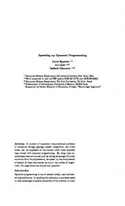
Fig. 4. Comparison of the cumulative running time of steps II and IV of our algorithm (marked x) with the running time of VA (marked o), for different values of k. Time is shown in arbitrary units on a logarithmic scale. Runs on the 1.5Mbp chromosome 4 of S. cerevisiae are in solid lines. Runs on the 22Mbp human Y-chromosome are in dotted lines. The roughly uniform difference between corresponding pairs of curves reflects a speedup factor of more than five.

We implemented both our improved LZ78-compressed algorithm from subsection 4.4 and classical VA in C++ and compared their execution times on a sequence of approximately 22,000,000 nucleotides from the human Y chromosome and on a sequence of approximately 1,500,000 nucleotides from chromosome 4 of S. Cerevisiae obtained from the UCSC genome database. The benchmarks were performed on a single processor of a SunFire V880 server with 8 UltraSPARC-IV processors and 16GB main memory. The implementation is just for calculating the probability of the most likely sequence of states, and does not trace back the optimal sequence itself. As we have seen, this is the time consuming part of the algorithm. We measured the running times for different values of k. In practice we found that the simple implementation of our algorithm (choosing all LZ78-words as good substrings) is a little slower than the regular VA implementation. However, an implementation of the refined algorithm (choosing just LZ78-words that appear as a prefix of more than k LZ78-words) performs roughly five times faster than VA. The fastest variant of our algorithm uses as good substrings all LZ78-words that appear as a prefix of more than a threshold of the LZ78-words. The optimal threshold is dynamically computed in the parsing step (III) of our algorithm. 14

Unlike the procedure described in section 4.3, this variant parses X into good substrings by applying the greedy procedure from section 4.3 to the entire sequence X, rather than to each LZ78word individually. As we explained in the previous sections we are only interested in the running time of the encoding and propagation steps (II and IV) since the combined parsing/dictionary-selections steps (I and III) may be performed in advance and are not repeated by the training and decoding algorithms. A comparison of the running time of steps II and IV of this variant to the running time of the corresponding calculation by VA is shown in Fig. 4. As k becomes larger, the optimal threshold and the number of good substrings decreases. Our algorithm performs faster than VA even for surprisingly large values of k. For example, for k = 60 our algorithm is roughly three times faster than VA. It is very likely that by using better heuristics for identifying good substrings one can get even faster implementations.

9

Conclusions and Future Work

In this paper we described a method for speeding up dynamic program algorithms used for solving HMM decoding and training. By utilizing repeated substrings in the observed input sequence, we presented the first provable speedups of the well known Viterbi algorithm. We based the identification of repeated substrings alternatively on the Four Russians method, and compression schemes such as RLE, LZ78, SLP and BPE. Our algorithms are faster than Viterbi in practice, and highly parallelizable. Naturally, it would be interesting to apply our results to other compression schemes. Other promising directions for future work include extending our results to higher order HMMs, HMMs with numerical observables [23], hierarchical HMMs, infinite alphabet size, and sparse transition matrices.

References 1. G. Benson A. Amir and M. Farach. Let sleeping files lie: Pattern matching in Z-compressed files. Journal of Comp. and Sys. Sciences, 52(2):299–307, 1996. 2. O. Agazzi and S. Kuo. HMM based optical character recognition in the presence of deterministic transformations. Pattern recognition, 26:1813–1826, 1993. 3. A. Apostolico, G.M. Landau, and S. Skiena. Matching for run length encoded strings. Journal of Complexity, 15:1:4–16, 1999. 4. O. Arbell, G. M. Landau, and J. Mitchell. Edit distance of run-length encoded strings. Information Processing Letters, 2001. 5. V.L. Arlazarov, E.A. Dinic, M.A. Kronrod, and I.A. Faradzev. On economic construction of the transitive closure of a directed graph. Soviet Math. Dokl., 11:1209–1210, 1975. 6. L.E. Baum. An inequality and associated maximization technique in statistical estimation for probabilistic functions of a Markov process. Inequalities, 3:1–8, 1972. 7. A.P. Bird. CpG-rich islands as gene markers in the vertebrate nucleus. Trends in Genetics, 3:342–347, 1987. 8. B. Brejova, D. G. Brown, and T. Vinar. Advances in hidden markov models for sequence annotation. In Bioinformatics Algorithms: Techniques and Applications. J. Wiley and Sons, 2007. To appear. 9. A. L. Buchsbaum and R. Giancarlo. Algorithmic aspects in speech recognition: An introduction. ACM Journal of Experimental Algorithms, 2:1, 1997. 10. H. Bunke and J. Csirik. An improved algorithm for computing the edit distance of run length coded strings. Information Processing Letters, 54:93–96, 1995. 11. P. C´egielski, I. Guessarian, Y. Lifshits, and Y. Matiyasevich. Window subsequence problems for compressed texts. In Proceedings of the 1st International Symposium Computer Science in Russia (CSR), pages 127–136, 2006. 12. T.M. Chan. All-pairs shortest paths with real weights in O(n3 /logn) time. In Proceedings of the 9th Workshop on Algorithms and Data Structures (WADS), pages 318–324, 2005. 13. T.M. Chan. More algorithms for all-pairs shortest paths in weighted graphs. In Proceedings of the 39th ACM Symposium on Theory of Computing (STOC), pages 590–598, 2007. 14. G.A. Churchill. Hidden Markov chains and the analysis of genome structure. Computers Chem., 16:107–115, 1992. 15. D. Coppersmith and S. Winograd. Matrix multiplication via arithmetical progressions. Journal of Symbolic Computation, 9:251–280, 1990.

15

16. M. Crochemore, G. Landau, and M. Ziv-Ukelson. A sub-quadratic sequence alignment algorithm for unrestricted cost matrices. In Proceedings of the 13th Annual ACM-SIAM Symposium on Discrete Algorithms (SODA), pages 679–688, 2002. 17. R. Durbin, S. Eddy, A. Krigh, and G. Mitcheson. Biological Sequence Analysis. Cambridge University Press, 1998. 18. G. Fettweis and H. Meyr. High-rate viterbi processor: A systolic array solution. IEEE Journal on Selected Areas in Communications, 8(8):1520–1534, 1990. 19. P. Gage. A new algorithm for data compression. The C Users Journal, 12(2), 1994. 20. J. Henderson, S. Salzberg, and K.H. Fasman. Finding genes in DNA with a hidden markov model. Journal of Computational Biology, 4(2):127–142, 1997. 21. J. Karkkainen, G. Navarro, and E. Ukkonen. Approximate string matching over Ziv-Lempel compressed text. Proceedings of the 11th Annual Symposium On Combinatorial Pattern Matching (CPM), pages 195–209, 2000. 22. J. Karkkainen and E. Ukkonen. Lempel-Ziv parsing and sublinear-size index structures for string matching. Proceedings of the 3rd South American Workshop on String Processing (WSP), pages 141–155, 1996. 23. J. Kleinberg. Bursty and hierarchical structure in streams. In Proceedings of the 8th ACM SIGKDD International Conference on Knowledge Discovery and Data Mining (KDD), pages 91–101, 2002. 24. A. Krogh, I.S. Mian, and D. Haussler. A hidden markov model that finds genes in E. Coli DNA. Technical report, University of California Santa Cruz, 1994. 25. Y. Lifshits. Processing compressed texts: A tractability border. In Proceedings of the 18th Annual Symposium On Combinatorial Pattern Matching (CPM), pages 228–240, 2007. 26. H.D. Lin and D.G. Messerschmitt. Algorithms and architectures for concurrent viterbi decoding. IEEE International Conference on Communications, 2:836–840, 1989. 27. V. Makinen, G. Navarro, and E. Ukkonen. Approximate matching of run-length compressed strings. Proceedings of the 12th Annual Symposium On Combinatorial Pattern Matching (CPM), pages 1–13, 1999. 28. U. Manber. A text compression scheme that allows fast searching directly in the compressed file. Proceedings of the 5th Annual Symposium On Combinatorial Pattern Matching (CPM), pages 31–49, 2001. 29. C. Manning and H. Schutze. Statistical Natural Language Processing. The MIT Press, 1999. 30. J. Mitchell. A geometric shortest path problem, with application to computing a longest common subsequence in run-length encoded strings. Technical Report, Dept. of Applied Mathematics, SUNY Stony Brook, 1997. 31. S. Mozes, O. Weimann, and M. Ziv-Ukelson. Speeding up HMM decoding and training by exploiting sequence repetitions. In Proc. 18th Annual Symposium On Combinatorial Pattern Matching (CPM), pages 4–15, 2007. 32. G. Navarro, T. Kida, M. Takeda, A. Shinohara, and S. Arikawa. Faster approximate string matching over compressed text. Proceedings of the Data Compression Conference (DCC), pages 459–468, 2001. 33. L. Pachter, M. Alexandersson, and S. Cawley. Applications of generalized pair hidden markov models to alignment and gene finding problems. In Proceedings of the 5th annual international conference on Computational biology (RECOMB), pages 241–248, 2001. 34. J.S. Pedersen and J. Hein. Gene finding with a hidden markov model of genome structure and evolution. Bioinformatics, 19(2):219–27, 2003. 35. W. Rytter. Application of Lempel-Ziv factorization to the approximation of grammar-based compression. Theoretical Computer Science, 302(1–3):211–222, 2003. 36. Y. Shibata, T. Kida, S. Fukamachi, M. Takeda, A. Shinohara, T. Shinohara, and S. Arikawa. Byte Pair encoding: A text compression scheme that accelerates pattern matching. Technical Report DOI-TR-161, Department of Informatics, Kyushu University, 1999. 37. Y. Shibata, T. Kida, S. Fukamachi, M. Takeda, A. Shinohara, T. Shinohara, and S. Arikawa. Speeding up pattern matching by text compression. Lecture Notes in Computer Science, 1767:306–315, 2000. 38. A. Siepel and D. Haussler. Computational identification of evolutionarily conserved exons. In Proceedings of the 8th annual international conference on Resaerch in computational molecular biology (RECOMB), pages 177–186, 2004. 39. V. Strassen. Gaussian elimination is not optimal. Numerische Mathematik, 13:354–356, 1969. 40. A. Viterbi. Error bounds for convolutional codes and an asymptotically optimal decoding algorithm. IEEE Transactions on Information Theory, IT-13:260–269, 1967. 41. J. Ziv and A. Lempel. On the complexity of finite sequences. IEEE Transactions on Information Theory, 22(1):75– 81, 1976. 42. J. Ziv and A. Lempel. A universal algorithm for sequential data compression. IEEE Transactions on Information Theory, 23(3):337–343, 1977.

16