SpiderBat: Augmenting Wireless Sensor Networks with Distance and ...

SpiderBat: Augmenting Wireless Sensor Networks with Distance and Angle Information∗ Georg Oberholzer, Philipp Sommer, and Roger Wattenhofer Computer Engineering and Networks Laboratory ETH Zurich, Switzerland

{ogeorg,sommer,wattenhofer}@tik.ee.ethz.ch ABSTRACT

1.

Having access to accurate position information is a key requirement for many wireless sensor network applications. We present the design, implementation and evaluation of SpiderBat, an ultrasound-based ranging platform designed to augment existing sensor nodes with distance and angle information. SpiderBat features independently controllable ultrasound transmitters and receivers, in all directions of the compass. Using a digital compass, nodes can learn about their orientation, and combine this information with distance and angle measurements using ultrasound. To the best of our knowledge, SpiderBat is the first ultrasound-based sensor node platform that can measure absolute angles between sensor nodes accurately. The availability of angle information enables us to estimate node positions with a precision in the order of a few centimeters. Moreover, our system allows to position nodes in multi-hop networks where pure distance-based algorithms must fail, in particular in sparse networks, with only a single anchor node. Furthermore, information on absolute node orientations makes it possible to detect whether two nodes are in line-of-sight. Consequently, we can detect the presence of obstacles and walls by looking at patterns in the received ultrasound signal.

In the last decade, the growing availability of positioning systems has spawned a market worth hundreds of billions of dollars. Today, almost every personal device features some positioning functionality, usually in the form of a receiver for the global positioning system (GPS). Inexpensive GPS receivers are used in hundreds of different applications, despite some limitations. Some of these GPS limitations may be fixed rather easily. Accuracy may for instance be improved by deploying additional groundbased reference stations. Unfortunately, other limitations remain, and hence positioning continues to be an exciting research topic. One of the main limitations of GPS is its lack of indoor localization support. This is particularly annoying in the sensor network context, first because many sensor networks will ultimately be deployed indoors, second because sensor data without position data is often meaningless. In particular, if sensors are mobile, or if the environment is changing, it will be important to know where sensor readings took place. Furthermore, location information may be beneficial in protocol design. Location information may for instance be used in the network layer, to facilitate routing decisions by means of a geographic routing algorithm [10, 11]. Or it may be used in the link layer, controlling interference by means of geographic information.

Categories and Subject Descriptors C.2.1 [Computer-Communication Networks]: Network Architecture and Design; B.m [Hardware]: Miscellaneous

General Terms Algorithms, Design, Experimentation

Keywords Wireless Sensor Networks, Localization, Ultrasound, Time Synchronization, Compass, Multipath ∗The authors of this paper are alphabetically ordered.

Permission to make digital or hard copies of all or part of this work for personal or classroom use is granted without fee provided that copies are not made or distributed for profit or commercial advantage and that copies bear this notice and the full citation on the first page. To copy otherwise, to republish, to post on servers or to redistribute to lists, requires prior specific permission and/or a fee. IPSN’11, April 12–14, 2011, Chicago, Illinois. Copyright 2011 ACM 978-1-4503-0512-9/11/04 ...$10.00.

INTRODUCTION

Ultrasound Positioning. One common technique in positioning is ultrasound, which is sound pressure at frequencies above the human hearing range. A main advantage of ultrasound (over GPS, and other alternative techniques) is its accuracy, providing distance precision in the order of a few millimeters. The location of a node can then be estimated using distances measured to a few neighbors. If nodes live in a plane, having accurate distance information to two neighbors is still not enough to position a node. Potentially, nodes can even iteratively figure out their location, starting with only a few anchor nodes that know their position. However, in order to achieve iterative positioning, the density of the network must be high, e.g., to allow for rigidity arguments [16]. Unfortunately, ultrasound technology is limited in range, and hence high node density is expensive. Furthermore, ultrasound sensors exhibit a limited beam angle and, therefore, the ranging capability suffers substantially at an increasing angle offset between transmitter and receiver. Another issue is that ultrasound distance measurements only work reliably if nodes are in line-of-sight.

Contributions. In this paper, we present SpiderBat, a novel ultrasound platform featuring four transmitters and four receivers (Section 2). As we will argue in the paper, having ultrasound hardware in all directions of the compass will solve the limited beam angle problem that previous ultrasound platforms (e.g. the Cricket nodes [22]) experience. In addition, thanks to multiple senders and receivers, we will have an increased accuracy. More importantly, the SpiderBat platform makes it possible to realize an old dream in sensor networks: Thanks to the eight ultrasound devices, we are able to estimate the distance and the direction of nodes up to a few degrees (Sections 3 and 4). Using both angle and distance information allows us to position a node accurately, even if the node only overhears a single anchor. Localization can also be done iteratively, i.e., we can estimate the position of several nodes in a network with only a single anchor, at minimal density. In order to achieve high accuracy, we must adapt positioning optimization techniques such that they can deal with angle information (Section 5). In addition, SpiderBat is equipped with a digital compass. As such, two nodes cannot only derive their relative angles, but also their absolute angles. Hence, it is possible that two nodes can detect that they are not communicating in line-of-sight, but that their signals are reflected by walls or obstacles. By looking at the second or third peak of an ultrasound signal, nodes can potentially learn about walls and obstacles in their environment (Section 7). Clearly, such advanced measurements need more elaborate signal processing capabilities compared to existing mote-class node architectures. However, one can easily imagine prospective applications for such a system. For example, one may just throw a few SpiderBat nodes into a dark building, and they will measure and report the interior architecture of the building to rescue teams. At this time, however, our platform is merely a proof of concept for such advanced application scenarios.

SpiderBat Ultrasound Platform Compass US TX (4x)

SYSTEM ARCHITECTURE

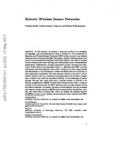
In this section, we present the hardware design of the SpiderBat platform. We designed SpiderBat as an ultrasound ranging board for existing sensor node platforms, e.g., the Crossbow TelosB or IRIS motes. The basic architecture of SpiderBat and its integration with the host node is depicted in Figure 1. The core of SpiderBat is a dedicated microcontroller that is used to control the transmit operation and to process the received signals. The ultrasound ranging board features four independently controllable ultrasound transmitters and four ultrasound receivers, which are placed alternately at the edges of the board, as shown in Figure 2. Using multiple transmitters and receivers has several advantages. On one hand we have an omnidirectional beam pattern, and on the other hand we are able to calculate the angle of arrival. Furthermore, a digital compass provides information about the absolute rotation of the node. The SpiderBat board has to be supplied with power by the sensor node, which allows to switch it off completely when not needed. The microcontroller is connected to the host node through the serial peripheral interface (SPI) and by two interrupt lines. In the remainder of this section, the individual building blocks of the SpiderBat prototype hardware are covered in more detail.

US RX (4x)

SPI IRQ IRQ

POWER

Wireless Sensor Node Sensors

Microcontroller Battery

Storage

Radio

Figure 1: The architecture of the SpiderBat system. The ultrasound ranging board is connected to the host node using standard interfaces (SPI, GPIO and Power).

2.1

Ultrasound Circuits

The ultrasound transceiver and receiver circuits have been designed with a focus on low complexity and cost. We used off-the-shelf ultrasound transducers with a center frequency of 40 kHz and a bandwidth of 1 kHz. To keep the complexity of transmitter and receiver circuits low, our system relies on the detection of the first peak of an ultrasound signal, rather than performing more sophisticated signal processing (e.g. pulse shaping using a chirp sequence). Furthermore, we decided in favor of separate ultrasound transmitters and receivers, rather than increasing the complexity by switching the circuits between receive and transmit mode. In the following, we highlight some key design aspects of the ultrasound transmitter and receiver circuits.

2.1.1

2.

Microcontroller

Ultrasound Transmit Circuit

To maximize the detection range, high output power is needed during the short time interval when the ultrasound transmitters are active (typically 250 µs). Therefore, a switched DC/DC converter is used to convert the supply voltage of the extension board (typically 3 V) to the operating voltage of the transmitters (12 V). It takes approximately 2 ms until the DC/DC converter reaches its nominal output voltage after startup. Since the transmitters require a stable output voltage, large capacitors are deployed upstream of each transmitter for power decoupling. The power supply of the transmitter circuits can be switched off completely to reduce the power consumption when operating the ultrasound board at low duty-cycles, e.g., when ultrasound pulses are transmitted every few seconds only. The microcontroller generating the output signal is operated at a much lower voltage than the ultrasound transmitters. Thus, an operation amplifier with a high supply voltage range is connected upstream of each transmitter. The ceramic ultrasound transmitter is driven at its resonance frequency (40 kHz) by a pulse-width modulation (PWM) output of the microcontroller.

2.1.2

Ultrasound Receive Circuit

Since the received signal is typically in the range of a few millivolts only, it needs to be amplified for reliable detection

RX INT RX RX ADC

Figure 3: Schematic view of the receiver circuit. The received ultrasound signal is amplified and fed to an analog-digital-converter input of the microcontroller (RX ADC). The comparator output triggers an interrupt when the received ultrasound signal exceeds the specified threshold (RX INT).

Figure 2: Top view of the SpiderBat ultrasound board with a digital compass attached. The board has a diameter of 6.5 centimeters (2.56 inches).

of ultrasound pulses. Therefore, each receiver is connected to three amplification stages, as shown in Figure 3. It is necessary to cascade the amplification due to the limited gain-bandwidth product (GBP) of the operation amplifiers. The ultrasound frequency of 40 kHz and the amplifiers having a GBP of 5 MHz result in a maximum gain of 42 dB per amplification stage. The first two amplification stages provide each an amplification of 21 dB. The third amplification stage is equipped with a digital potentiometer to adjust the detection threshold and to prevent saturation of the sampled signal. Thus, the overall amplification gain is dynamically adjustable in the range between 58 dB and 75 dB. Finally, the amplified signal is rectified and low-pass filtered. The parameters of the low-pass filter are chosen such that false detections are prevented and the signal raise is not delayed significantly. The amplified receiver signal is connected to an analogdigital-converter (ADC) input pin of the microcontroller, which allows to sample the received ultrasound signal. To unburden the microcontroller from sampling the input signal continuously, a comparator circuit is used to indicate the presence of ultrasound signals. This detection signal is connected to a capture input of the microcontroller, which provides a hardware interrupt with an accurate timestamp for the first received ultrasound peak. Thus, our architecture offers the flexibility to choose between low-power operation (peak detection in hardware) and continuous sampling of the input signal for more advanced application scenarios.

2.2

Data Processing

The SpiderBat board features a MSP430F2274 low-power microcontroller from TI with 1 kByte RAM and 32 kByte ROM. We decided to include a dedicated microcontroller since most existing sensor node platforms do not provide enough free timers or I/O pins to operate the ultrasound hardware. Furthermore, performing an ultrasound transmit or receive operation is highly time critical. Having this functionality implemented on the sensor node itself would possibly interfere with other time critical operations, e.g.,

controlling the radio transceiver. The MSP430F2274 provides two hardware timers, each having two independent inputs for time capture and two outputs to generate a PWM signal to control the transmitters. The comparator output of each receiver is connected to a timer input, while the amplified signals of the receivers are connected to the 10-bit ADC input pins. Moreover, we use a Honeywell HMC6352 2-axis digital compass to determine the absolute node orientation. It is connected using a 4-pin socket on the top side of the SpiderBat board. The current heading value from the compass can be read using the I2 C bus.

2.3

Sensor Node Interface

The SpiderBat ultrasound board can be connected to different sensor node platforms using a 16-pin connector. Power has to be provided by the host node. Table 1 reports the measured power consumption for different operation modes of the extension board. The host node (master) controls the ultrasound board (slave) using the SPI bus. Each data transfer is started by a command byte that determines the operation type. The microcontroller on the ultrasound board exposes a register address space for read and write access by the host node. This allows the host node to configure several parameters of the ultrasound ranging operation and to read back the measurement results. Furthermore, two interrupt lines, one for each direction, are used for mutual notifications between the host node and the ultrasound board. This unburdens both sides from having to poll for status changes. While the extension board is busy with a receive operation, the host node can remain in low-power state. Once the receive operation is completed, the host will be notified by an interrupt. Similarly, the microcontroller on the SpiderBat board can remain in low-power state when no ultrasound ranging operation is active, otherwise it can be woken up. Operation mode Idle Ultrasound receive (min/max gain) Ultrasound transmission (peak current)

Current 320 µA 4.68 / 4.76 mA up to 100 mA

Table 1: Current consumption of the ultrasound board for different operation modes. The ultrasound receive and transmit circuits can be switched off completely from the supply, which allows to dutycycle the extension board when battery-powered.

Tstart Sender

Treceive

Tultrasound

Tdetection

Radio

Receiver

Radio t

∆tradio ∆toffset ∆tdelay

∆tflight

Figure 4: Timeline of events during a single ultrasound measurement between a sender and receiver node. The measurement is initiated by a radio packet, which is followed by an ultrasound pulse.

3.

ULTRASOUND RANGING

An ultrasound ranging operation is always unidirectional. The sender node initiates a single measurement by broadcasting a radio packet followed by an ultrasound pulse, while nearby nodes listen for incoming ultrasound waves. To measure the time difference of arrival between the radio packet and the ultrasound pulse accurately, both the radio and ultrasound transmissions have to be started concurrently, e.g., as with Cricket [22]. However, in our implementation the ultrasound transmission is started a fixed time interval after the ranging procedure has been initiated by the sender node. Shifting the start of a radio transmission has several advantages in practice. First, it is not necessary to modify the radio driver to start the ultrasound transmission at the same time as the radio transmission. Depending on the radio chip this might even not be possible since we do not have control over the precise timing. Second, the received radio packet can be processed in the application layer before the ultrasound pulse reaches the receiver. This enables the receiver node to start the ultrasound receivers only when necessary, providing a low duty-cycle operation of the extension board. A similar approach is also used on the Medusa platform [24], where the ultrasound transmission is started when the radio transmission ends. Figure 4 shows the timeline of events during a typical ranging procedure. First, the sender node configures the ultrasound board for a transmit operation. After a certain delay, which is required to ramp up the power supply for the transmission section, the node triggers an interrupt and stores Tstart , the corresponding local time of this event. It then broadcasts a radio packet containing a measurement request for all other nodes in the sender’s radio communication range. This packet is timestamped at the MAC layer [14] on both the sender and receiver, and contains the interval elapsed since Tstart . Next, the SpiderBat board starts the ultrasound transmission after ∆tdelay . This delay has to be larger than the total radio communication delay ∆tradio , which highly depends on the delay introduced by the MAC layer protocol. We use ∆tdelay = 20 ms in our implementation. Nodes that have received the radio packet power up the ultrasound receivers on the extension board. At the same time, an interrupt is triggered to initiate a time of arrival measurement on the extension board and Treceive , the local time of this event, is stored. With the help of sender-receiver time synchronization [12], the receiver can determine Tstart , the start of the transmission in the receiver’s local time.

Furthermore, the receiver calculates the time difference ∆toffset = Treceive − Tstart

(1)

that has passed between the start of the ranging procedure on the sender side (Tstart ) and the start of the ultrasound measurement on the receiver side (Treceive ). When the two nodes are rather close, e.g., less than one meter apart, this delay can exceed the actual time of flight of the ultrasound message. The receiver node is interrupted by the extension board when at least one receiver has detected the ultrasound signal or the receive timeout has expired. Finally, the receiver node is able to calculate the time of flight of the ultrasound pulse as follows: ∆tflight = Tdetection − Treceive − (∆tdelay − ∆toffset )

(2)

The corresponding distance d between the sender and receiver node follows directly by multiplication with the propagation speed c of ultrasound: d = c · ∆tflight

3.1

(3)

Clock Synchronization

Since the radio communication delay is measured using the local clock of the host node, and the time of arrival is calculated at the ultrasound board, it is important that the clock drift between the two microcontrollers is kept minimal. If possible, they should both be sourced by the same clock to eliminate errors due to clock drift. Furthermore, the accuracy of a time of arrival measurement depends on the clock granularity. The local hardware clock of the TelosB motes, for example, is sourced by a 32 kHz crystal, which corresponds to a quantization error of roughly 1 cm. Other mote platforms, e.g, the IRIS nodes, have a hardware clock sourced by a crystal quartz, which provides a stable 1 MHz clock. Since we are only interested in the time difference of arrival and not the absolute arrival time, synchronization of clock offsets between neighboring nodes is not required with our approach. However, clock drift between different nodes affects the accuracy of ultrasound ranging since the delay before transmitting the ultrasound pulse (∆tdelay ) is measured using the local hardware clock as a reference. Quartz crystals used as clock sources on mote-class hardware exhibit clock drifts up to 50 ppm. Thus, when having a worst-case clock drift of 100 ppm between two neighbors, the estimation of ∆tdelay at the receiver is off by two clock ticks, which corresponds to a distance of approximately 0.7 mm at 1 MHz

0.006 North

100

0.005

East

0.004

0 100

0.003 South

Measurement error [m]

0 100

0.002

0 100

0.000

West

0.001

1

2

3

4

5

6

7 9 8 Distance [m]

10

11

12

13

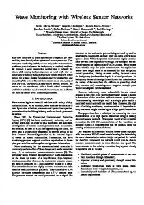
Figure 5: Standard deviation of the ultrasound ranging error at different distances.

clock speed. However, the estimation of the time of flight depends solely on the clock drift of the receiving node. In the worst-case of 50 ppm drift, this contributes two clock ticks to the measurement error at the maximum ranging distance of 15 m. Therefore, not synchronizing local clocks by running a dedicated time synchronization protocol introduces a ranging error of only 1.4 mm in the worst-case.

3.2

0 2.6

14

Accuracy of Distance Measurements

In order to evaluate the accuracy of distance measurements with SpiderBat, we placed two sensor nodes equipped with an ultrasound board a certain distance apart. The receiver node records the timestamp when the peak detection signal is triggered for each ultrasound receiver. Since we were not able to measure ground truth distances within submillimeter accuracy, we are mainly interested in the variance of the distance estimation. The standard deviation of the ranging error is 0.31 mm at a distance of 1 m and 5.39 mm at the distance of 14 m, as shown in Figure 5. The absolute error when compared to the distances measured with a measuring tape, is in the order of a few millimeters. The received signal strength of ultrasound pulses decreases with increasing distance from the transmitter. Thus, it becomes more likely that the exact start of the ultrasound pulse is missed since the amplitude of the first few wavelengths is below the threshold value of the comparator. Figure 6 shows the distribution of the time of flight measurements for all four ultrasound receivers at a distance of 1 m. Since the northbound receiver points directly towards the transmitter, it detects incoming pulses first, followed by the eastbound and westbound receivers. Eventually, also the southbound receiver detects the pulse. However, we observe that receivers North and South frequently fail to detect the first peak, since the ultrasound signal strength remains slightly below the comparator threshold for the first peak. Instead, they catch a subsequent peak in the signal arriving at a multiple of the wavelength (25 µs) later. However, when sampling the ultrasound signal strength immediately after detecting a peak, a strong correlation between the signal strength and the real arrival time of the first peak is observed.

2.7

2.8 Time of flight [ms]

2.9

3.0

Figure 6: Histogram of time of flight measurements for each ultrasound receiver at a distance of 1 m from the sender node.

4.

ANGLE OF ARRIVAL ESTIMATION

The spatial displacement of the different ultrasound receivers on the SpiderBat platform can be leveraged to estimate the angle of arrival of the corresponding ultrasound wave. The relatively slow propagation speed of ultrasound and the board dimensions result in a difference in the time of arrival at the different receivers, which can be measured using the hardware-based peak detection mechanism described in Section 2. In this section, we show how SpiderBat can combine information from multiple ultrasound receivers to estimate the angle of arrival. Furthermore, we evaluate the accuracy of this approach in practice. The ultrasound receivers on the SpiderBat board have a main beam width of roughly 30◦ and two side lobes at −45◦ and +45◦ . Thus, assuming a certain ultrasound receiver is pointing towards 0◦ , it can cover an area between -45◦ and +45◦ . However, even a signal arriving from the opposite direction than the receivers orientation can be detected, but the signal strength is much lower. If a signal origins from outside this sector, it is received at another receiver first. Consequently, knowing which receiver has detected the pulse first limits the uncertainty in the angle of arrival to a sector of 90 degrees only. Furthermore, due to the symmetric shape of the extension board, the arrival time of an ultrasound pulse at different ultrasound receivers can be used to calculate the angle of arrival. Depending on the angle of the incident wave and the signal strength of the ultrasound signal, we can detect a pulse at multiple receivers. Figure 7 shows a measurement of the received signal at all four receivers. We can clearly distinguish the detection of the first peak of the ultrasound signal at different receivers. If at least three receivers have detected the incoming pulse, as shown in Figure 8, this results in two mutual differences (∆t1 and ∆t2 ) between the time of arrival at the three receivers. By multiplication with the speed of sound c, we get two corresponding distances l1 and l2 as follows: l1 l2

= c · ∆t1 = c · ∆t2

(4) (5)

North

3 2 1 0

East

3 2 1 0

South

3 2 1 0

West

3 2 1 0

0.0

0.5

1.0

1.5

2.0

3.0

2.5

Time [ms]

Figure 7: Measurement of the amplified ultrasound signal (RX ADC) at all four ultrasound receivers. The direct ultrasound path reaches the receiving node from the north direction, but additional signal paths are visible too. Furthermore, the plot shows the status of the peak detection signal (RX INT) for each receiver.

α

0 rtx

N r π 4

N

d 0 rrx

αtx

−α

r αrx

l2 d

d l1

π 4

−α

Figure 8: Calculation of the angle of arrival based on three timestamps provides an unambiguous solution for the estimated angle α of the incoming wave.

Applying basic trigonometry, we get Equations 6 and 7, which can be combined into Equation 8. Since the spacing d between the ultrasound receivers is equal, the angle of arrival α depends on the differences in the time of arrival only. π −α = 4   π cos −α = 4 sin





α

=

l1 c · ∆t1 = d d l2 c · ∆t2 = d d   π ∆t1 − arctan 4 ∆t2

(6) (7) (8)

Even if a pulse is detected by only two neighboring receivers, the extension board can still calculate the angle of arrival according to Equations 6 or 7. Unfortunately, having only a single time difference ∆t1 results in two possible candidates α and α0 for the angle of arrival. However, if only two sensors have detected the signal, we can assume that the signal originates in the sector covered by these two sensors. This leads to an unambiguous solution for the angle of arrival α, because otherwise, it is very likely that at least another sensor would have detected the signal too.

Figure 9: Distance measurement between a sender node (left) and a receiver node (right). The distance measurement is performed between the closest transmitter-receiver pair.

4.1

Distance Correction

The time of flight of ultrasound pulses is always measured between the ultrasound transmitter and receiver pair of minimum distance, as depicted in Figure 9. However, this distance has to be corrected with the board radius r in order to position the center of the board correctly. Since the ultrasound hardware is located at the edges of the board, the real distance depends also on the angle between the nodes, on both the transmitter and receiver side. To get an accurate distance between the two nodes, additional angle information is required. Otherwise, an uncertainty in the order of the board radius remains. If the angles αrx and αtx are known, Equations 9 and 10 can be used to calculate the dis0 tance correction term for the transmitter rtx and receiver 0 rrx , respectively.

( 0 rrx

r · |sin (αrx )|

, αrx ∈ [ 3π 4

5π [ 4

∪ [ 7π , 2π[ ∪ [0, π4 [ 4

= r · |cos (αrx )| αrx ∈ [ π4 ,

3π [ 4

∪ [ 5π , 4

7π [ 4

(9)

0 rtx


 r · sin αtx − π4 αtx ∈ [ π2 , π[ ∪ [ 3π , 2π[ 2 =  r · cos α − π
α ∈ [0, π [ ∪ [π, 3π [ tx tx 4 2 2

(10)

3 d3 90

Measurement [deg]

d1 60

d1

2

α1

d2

α2 2 d2

45

30

Figure 11: Relying on distance information only (left) requires more anchor nodes to position an unknown node (indicated by the cross) than combining distance with angle measurements (right).

15

0 0

15

30 60 45 Angle of arrival [deg]

75

90

5. Figure 10: Estimation of the angle of arrival using information from multiple receivers. Error bars indicate the standard deviation of the measurement.

The distance correction term is in the range between 2.8 and 4 cm for the SpiderBat hardware. If we assume uniform distribution of the angle of arrival, the expected value of the = 3.6 cm, which is the correction correction term is r· cos(π/4) π/4 term being applied in the absence of angle information, e.g., when a pulse is only detected by a single receiver.

4.2

1

1

75

Accuracy of Angle Measurements

We performed a series of measurements to evaluate the accuracy of angle estimation using multiple receivers. Two SpiderBat boards were placed at a fixed distance of one meter such that one ultrasound transmitter points directly towards the receiver node on the other board. During the experiments, the receiving board was rotated step-by-step to measure the time of arrival at different incident angles (0◦ , 15◦ , 30◦ , 45◦ , 60◦ , 75◦ and 90◦ ). Based on the time of arrival information, we calculated an estimation for the current angle of arrival. Figure 10 shows the mean and the standard deviation of the calculated angle of the incident ultrasound wave at different angles. As we can see from the measurement results, the estimation error depends on the particular angle of the incident wave. We observe a measurement error of less than 2◦ when the incident wave hits the receiver at the main lobe (0◦ or 90◦ ) or at the peak of its side lobes (45◦ ). In all other cases (15◦ , 30◦ , 60◦ and 75◦ ), the signal strength of the received ultrasound pulse will be significantly lower. Thus, it can happen that the first peak will not trigger the detection signal, but only the second or even third peak will do so. This results in a measurement error in the time of arrival, and thus, also in the estimation of the incident angle. Clearly, the performance of angle measurements could be improved by adding more ultrasound receivers. However, we observe that by using only four receivers, the mean error in our measurements is below 5◦ for short distances. Furthermore, the measurements indicate that by applying a non-linear correction function, we can further improve the accuracy of angle measurements with the SpiderBat platform.

MULTI-HOP POSITIONING

Localization algorithms have been studied extensively in the context of wireless sensor networks, both in theory [17, 5, 3, 21] and practice [23, 15]. Many existing approaches assume the presence of one or multiple nodes, so called beacons or anchors, which have known positions [9, 2, 25, 32]. By using iterative or optimization techniques, a positioning algorithm will assign positions to non-anchor nodes. Anchorfree ranging algorithms do not rely on anchors nodes, but obtain position information relative to their neighbors. Rangebased localization algorithms utilize distance or angle information acquired by specialized hardware [22, 24, 18, 29, 7], while range-free localization algorithms [26, 19] do utilize connectivity information between nodes only, at the cost of reduced accuracy. In the remainder of this section, we discuss the adaptation of positioning techniques for leveraging distance, angle and compass information provided by the SpiderBat architecture. Assuming nodes are positioned in a two-dimensional plane, the position of each node contributes two unknown variables x and y to the localization problem. Hence, to solve the localization problem unambiguously, two linearly independent equations are required for each node. In range-based localization, the set of equations usually consists of the distances between the nodes and several anchor nodes. Relying on distances between nodes only, a simple setup with three anchor nodes, as shown in Figure 11, requires three distance measurements to determine the position of a non-anchor node. However, additional information about the angle towards a not positioned node, as provided by the SpiderBat platform, satisfies to solve the problem unambiguously with only two receivers. Basically, even a single measurement for both distance and angle to an anchor node is enough to determine the position of a not positioned node. However, measurements to additional anchor nodes improve the quality of the positioning. Since the angle of arrival αij is measured relative to node i’s absolute rotation, we need to convert it into a common coordinate system. This can be accomplished by comparing αij to the angle αji of an anchor node j, which is equal up to 180◦ for line-of-sight ultrasound paths. Thus, we learn the absolute orientation of node i. Alternatively, we can also use the absolute node orientation φi , provided by the node’s compass, to convert relative angles into absolute angles. By comparing the results of these two approaches, we can check the solution for plausibility, e.g., to detect a non line-of-sight path, as discussed later in Section 7.

5.1

Positioning Algorithm

In the following, we describe a centralized positioning algorithm that employs information about distance and angles. We assume that the algorithm has access to all measurement data (distances and/or angles) gathered at the nodes in the network. This can be achieved by letting nodes forward distance and angle measurements along a collection tree to the base station. The positioning algorithm itself consists of two separate phases. In the first phase, each node is assigned an initial placement within the coordinate system. Then, the node positions are iteratively optimized using the method of least squares.

5.1.1

Initial Node Placement

In the first phase, we assign each not positioned node the anchor node with the smallest hop distance. This is motivated by the fact that each ultrasound measurement introduces a certain error in the position estimation. Thus, the positioning accuracy decreases with increasing hop count from the anchor node. If two anchor nodes have equal hop count, we further take into account the accumulated distance to the anchor node, since the error in the ultrasound distance estimation increases by distance too. By doing so, we construct several trees, each rooted at the corresponding anchor node. By processing these trees in a top-down manner, we obtain an initial position estimate for each child node j based on the distance dij and the angle αij to its parent i in the tree, which is calculated according to Equation 11.



xj yj



 =

xi yi



 + dij ·

cos(αij + φi ) sin(αij + φi )

 (11)

The initial node placement requires the availability of angle and distance information to at least one neighbor. As discussed before, angle measurements have higher requirements than distance measurements since at least two ultrasound receivers need to detect the signal. Otherwise, we only know the distance to the node and in which sector of 90 degrees the signal has originated. In such a case, we need to have another distance measurement to a neighbor to perform the initial placement of the node.

5.1.2

Least Mean Square Method

In the first phase of the positioning algorithm, we have not yet taken into account all available measurements between the nodes. In general, distance estimations are usually more accurate than angle estimations and the location error introduced by an inaccurate angle estimation is larger than by an inaccurate distance estimation. Thus, we employ the method of least mean squares (LMS) to improve the location accuracy further by taking into account all available distance information. The squared distance error of node i is given by Equation 13, where dij is the measured distance between node i and j, and dˆij is the distance according to the current node placement (xi , yi ) and (xj , yj ). dˆij ei

=

p

=

X

(xi − xj )2 + (yi − yj )2 (dij − dˆij )2

(12) (13)

j

The least mean squares (LMS) method is a steepest gra-

dient descent method, which iteratively reduces the sum of the squared distance errors ei . Equations 14 and 15 show the derivation of the distance error with respect to the x and y coordinate. ∂ei ∂xi ∂ei ∂yi

= −

X  dij − dˆij  2

dˆij

j

= −

(xi − xj )

X  dij − dˆij  2

dˆij

j

(yi − yj )

(14)

(15)

The LMS algorithm iteratively updates the current position of the nodes in every step according to Equations 16 and 17, where µ < 1 denotes the learning rate.



xi,k+1

= xi,k − µ

∂ei (x, yi,k ) ∂x x=x

(16) i,k



yi,k+1

∂ei (xi,k , y) = yi,k − µ ∂y y=y

(17)

i,k

The algorithm terminates after a fixed number of iterations or as soon as the sum of the square errors does not decrease significantly any further, which indicates that the optimal positioning for the given distance measurements has been found.

6.

EVALUATION

In order to evaluate the performance of the SpiderBat platform for positioning in wireless sensor networks, we implemented a localization application in TinyOS. In our prototype implementation, the SpiderBat extension board is connected to a custom node platform with the Atmel ZigBit900 module at its core. The ZigBit900 module combines an Atmega1281 microcontroller (128 kByte of flash memory, 8 kByte of RAM) and a RF212 radio transceiver for the 900 MHz ISM band in a single enclosure. The external quartz of the radio transceiver provides an accurate 1 MHz clock output, which is used as the clock source for the host sensor node and the ultrasound board. The host node and the ultrasound board are powered by two standard AA size rechargeable batteries. We produced four SpiderBat boards for evaluation purposes, limiting the size of our testbed to four nodes.

6.1

Experimental Setup

The indoor experiments were set up in a gym in order to have all four nodes contained within a large area without any obstacles. We placed four nodes in an area of 10x6 m, approximately 1.5 m above ground. The outdoor testbed is located on a sports ground, where we placed four nodes in an area of 10x5 m, approximately 20 cm above ground. An ultrasound ranging operation, as described in Section 3, is initiated by each node once within each measurement round. The receiving nodes report their estimated distance, angle of arrival and compass information to the base station, where the data was collected with a PC. Since all nodes are within the radio communication range of the base station, the use of a collection protocol was not necessary in this setup. After each round, we use the measurement data from all four nodes as input for the localization algorithm.

3

3 Node 2

Node 2 2

1

Node 1

Y−Position [m]

Y−Position [m]

2

Node 3

0 −1

1

Node 1

Node 3

0 −1

Node 4

Node 4

−2 −3 0

−2

1

2

3

4 5 6 X−Position [m]

7

8

9

−3 0

10

(a) indoor setup: initial positioning

3

4 5 6 X−Position [m]

7

8

9

10

2 Node 1

Node 2

1

0

0

−1

−1 Y−Position [m]

Y−Position [m]

2

(b) indoor setup: with LMS

2 1

1

−2 −3 −4

Node 3

−5

−3 −4

−6

−7

−7 4

5

6

Node 3

−5

Node 4

3

Node 1

−2

−6

−8 −8 −7 −6 −5 −4 −3 −2 −1 0 1 2 X−Position [m]

Node 2

7

8

Node 4

−8 −8 −7 −6 −5 −4 −3 −2 −1 0 1 2 X−Position [m]

(c) outdoor setup: initial positioning

3

4

5

6

7

8

(d) outdoor setup: with LMS

Figure 12: Experimental results for the indoor and outdoor settings: Initial position estimates are based on the distance and angle to the closest neighbor (plots (a) and (c)). Post-processing of position estimates is done using the method of least mean squares (LMS) (plots (b) and (d)). The average position over all ultrasound measurements for each node is indicated with a circle, the cross marker indicates the node position measured using a reference tape.

6.2

Experimental Results

During all measurements, Node 1 is an anchor node with a known orientation and position at the origin of the coordinate system. The positions of all other nodes are not known a priori, they are determined using mutual distance and angle information to neighboring nodes. In a first step, we locate the nodes using angle and distance estimates to their closest neighbor only. Next, we apply the LMS algorithm, which takes into account distance estimates between all neighboring nodes. The estimated positions of the nodes are shown in Figure 12 and the measurement results are summarized in Table 2. The node positions gathered with a measuring tape are depicted in Figure 12 for reference.

6.2.1

Indoor Experiments

We observed that nodes have both distance and angular measurement only to nodes in close proximity, e.g., Node 2 can measure both angle and distance to Node 1 and 3, but not to Node 4. However, distance information may still be available to nodes that are further away. In the indoor setup, the standard deviation of the localization error is 15.5 cm in the worst-case, which is reduced to 5.7 cm by applying

the method of least squares for all known distances between nodes. Furthermore, the measurement results show that the positioning error increases with every hop, as each localization is based on noisy position estimates of the previous node. Although our setup consists of a single anchor node only, we conclude that the SpiderBat platform allows us to localize all three nodes within a few centimeters in an indoor environment. Clearly, adding additional anchor nodes, e.g. setting Node 4 as an anchor too, could further reduce the localization error for non-anchor nodes.

6.2.2

Outdoor Experiments

Although SpiderBat is mainly targeted at indoor applications, we performed an outdoor experiment on a sports ground. The measurement results indicate that the positioning is less accurate compared to the indoor setting. Since distances between nodes are larger than in the indoor experiments, nodes frequently fail to measure an angle of arrival due to the effects described in Section 4. Furthermore, ultrasound waves are susceptible to small air disturbances and changes in the ambient temperature, which can impair the measurement accuracy outdoors.

Node 1 Positioning Error (std. dev) initial positioning LMS method

– –

Indoor Setup Node 2 Node 3

Node 4

Node 1

2.0 cm 2.2 cm

15.5 cm 5.7 cm

– –

8.3 cm 4.2 cm

Outdoor Setup Node 2 Node 3

Node 4

58.2 cm 37.7 cm

61.2 cm 51.6 cm

51.5 cm 36.2 cm

Table 2: Summary of measurement results for the indoor and outdoor experiments.

Receiver North [V]

3

φB

B’

2

αBA 1

B

Receiver North [V]

0 3

2

φA αAB

1

0

C

0

1

2

3

4

5

6 Time [ms]

7

8

9

10

11

12

Figure 13: Multipath effects measured at a single ultrasound receiver: The line-of-sight signal reaches the receiver after about 1.8 ms. The second peak is a reflection at a near-by wall and is detected at around 9.7 ms (top). Since the line-of-sight path is obstructed in the second measurement, only the reflected path is above the detection threshold (bottom).

7.

NON LINE-OF-SIGHT PROPAGATION

Ultrasound signals cannot penetrate solid objects, they rather get reflected by them. If the line-of-sight path between two nodes is obstructed, the signal may take a different path including reflections at walls or objects. More generally, a receiver will usually receive the same ultrasound transmission several times. In wireless communication this is a notorious phenomenon, known as multipath propagation. These multipath effects are present in Figure 7 already. Figure 13 presents a different example, with only one receiver, using a different horizontal scale. In the current implementation of the SpiderBat hardware, an interrupt is triggered when the received ultrasound signal exceeds a certain threshold. As shown in Figure 13, sampling the incoming signal during the reception of a pulse reveals valuable information. Due to the limited memory of the microcontroller, only a small amount of samples can be recorded for further processing, e.g., 12 ms of a signal of one particular receiver at a sampling frequency of 80 kHz. As seen in the example of Figure 13, indirect paths can be considerably longer than line-of-sight paths. Also, the signal of indirect paths will usually be weaker, and at some point hard to detect. In obstructed environments it is important to detect that two nodes are not in line-of-sight. If not, a positioning algorithm may severely misplace some of the nodes. Having a dense enough network, with distance measurements between many pairs of nodes, a smart positioning algorithm may detect that indeed some distance measurements will be too large to be possible in Euclidean geometry, for instance because the triangle inequality is violated.

A

Figure 14: Since there is no line-of-sight path between A and B, only the ultrasound signal reflected by a near-by wall can be received. Thus, a generic trilateration positioning algorithm will erroneously confer that B is located at position B’. It may then ignore these wrong distances and just run the algorithm on the reliable (short) distance measurements. Thanks to the digital compass and the availability of angle information, SpiderBat has the advantage of absolute angle information, which can be used to detect indirect paths more easily. If two nodes are in line-of-sight, they will receive their respective signals at opposite angles, i.e., with an offset of about 180◦ . Consequently, we know that two nodes i and j are in lineof-sight if the following equation holds: 0 0 φi + αij = φj + αji −π±

(18) 0 αij

is the where φi is the absolute orientation of node i, angle of the signal from node j relative to node i, and  is the total measurement error. On most non-trivial indirect paths, such as the one in Figure 14, this is not the case. However, not all indirect paths can be identified using this approach. For instance, if a signal gets reflected at two parallel walls, Equation 18 will still be fulfilled. On the other hand, at the price of a higher node density, we may not need a digital compass. For instance, when having three nodes, each node measures the angle between its two neighbors (of the two possible angles we choose the smaller one). Then, if all pairs of nodes are in line-of-sight, the three measured angles should sum up to 180◦ . If they deviate drastically, we can conclude that at least two nodes are not in line-of-sight. Furthermore, SpiderBat may also be used to learn about the environment of a node by sending out an ultrasound pulse and analyzing the echo from nearby walls or obstacles. Apart from the technical challenges to implement an echo, some other difficulties have to be mastered before one can correctly position walls and obstacles. For instance, objects need to have a certain dimension in order to be visible from

multiple vantage points. At this stage, detecting many small obstacles seems beyond the possibilities of the SpiderBat approach. However, in the future, one may hope of throwing a few SpiderBat-like nodes into a dark building, learning its architecture using a wireless sensor network.

8.

RELATED WORK

Node positioning in wireless sensor networks has been studied extensively during the last decade. In this section, we compare our approach to other localization techniques. Fixed Positioning. For some sensor network deployments, learning the position of a node is trivial: we just make a note where we put the sensor node during the initial deployment phase. This is a common practice in environmental or heritage monitoring, where each node has to be carefully placed to gain meaningful measurement data, e.g., [4, 6]. However, this approach might fail in many other scenarios. The sensor node might move over time because of external influences, e.g., since the object where the sensor is attached may be in continuous movement. Also, it might simply be too time consuming to place the nodes manually, or nodes are deployed in an environment that is too dangerous for human interaction. For many applications a single positioning phase is required just once after the nodes are deployed. Adding dedicated hardware for the positioning may increase the total cost and energy consumption of the node. Passive localization systems, e.g., [28], exhibit spatio-temporal properties of external events to localize nodes in the network. While being energy efficient and low-cost, such systems are generally outperformed in terms of accuracy by systems with dedicated ranging hardware. Acoustic Positioning. Various different platforms for acoustic source localization applications have been proposed. The ENSBox [8] is a distributed localization and processing platform used for example in habitat monitoring [1]. It features a microphone array for acoustic source localization and is built around an powerful ARM/Linux core, which allows for sophisticated signal processing. Furthermore, the platform can be self-calibrated using wide-band chirp signals and digital signal processing. The countersniper system proposed in [27] is able to detect the location of a sniper in urban terrain. A gunshot produces a short, easily distinguishable pulse, which is detected by an array of microphones. The hardware is optimized for high-frequency signal processing. Nodes need highly synchronized clocks to estimate the position of the sniper accurately. Ultrasound Positioning. Ultrasound is a common technique to measure distances and to locate objects or people. A major advantage compared to acoustic positioning is the operation outside the range of human hearing, which allows to use ultrasound for “stealth” applications. The Bat indoor location system [9] uses active ultrasound tags, the so-called bats, which are attached to an object of interest or a person. Ultrasound receivers are mounted on the ceiling, measuring the time of flight of an ultrasound pulse emitted by a bat. Trilateration is used to determine the position of the corresponding tag. The Cricket platform [22] has introduced ultrasound ranging into the field of wireless sensor networks. It combines a low-power sensor node with an ultrasound transmitter and

receiver. Cricket exploits the substantial difference in propagation speeds between radio and ultrasound signals to measure the distance between two nodes. Having only a single transmitter/receiver pair, ranging capabilities of the Cricket platform are limited to one sector. Commonly, and similarly to the Bat system, beacon nodes are mounted on the ceiling to track listeners deployed on the floor. This setup allows to track mobile nodes in an indoor environment with an accuracy of a few centimeters. The Calamari platform [30] features a reflective cone on top of the ultrasound transceiver, yielding an omnidirectional beam pattern at the cost of a reduced range. Similar to our approach, Medusa [24] uses an extension board containing an array of four ultrasound receiver and transmitter pairs, which cover the hemisphere above the node. Upon detection of an ultrasound signal on a receiver, an external interrupt pin of the microcontroller is triggered. However, the Atmega128L microcontroller does not provide hardware capture for multiple interrupt signals, while this is possible with the SpiderBat platform. RF-based positioning. While acoustic localization provides precise distance measurements within a few centimeters, its range is limited to a few meters. A rich body of prior work was done on mere RF-based ranging, e.g., [2, 32, 31, 33]. The propagation speed of radio signals is orders of magnitude higher than for ultrasound. Therefore, specialized hardware is required to measure time difference of arrival for electromagnetic waves. Also, it has been shown that RSSI is a bad indicator for the distance in multi-path environments, e.g., [20]. Radio interferometric location is based on the superposition of two radio waves, transmitted at slightly different frequencies by two nodes [15]. The relative phase offset of the radio signal at two receivers can be used to calculate the distance between the nodes. However, the application of radio interferometry requires high node density in the network. RF Doppler shifts measured on the Mica2 platform have been used to track mobile nodes [13].

9.

CONCLUSIONS

This paper presents the design and implementation of SpiderBat, a novel hardware platform for ultrasound ranging applications. SpiderBat is designed as an extension board for wireless sensor nodes, with a focus on the low computation complexity of sensor nodes and with energy efficiency operation in mind. Multiple ultrasound receivers and transmitters allow SpiderBat to measure distances and angles between nodes accurately. Our experiments have shown that the distance between two nodes can be determined in the range of a few millimeters to a few centimeters, whereas the accuracy of the angle of arrival lies within a few degrees, depending on the actual angle of arrival and distance between the two nodes. The combination of angle of arrival and orientation provided by an on-board digital compass provides several advantages over existing platforms. With such a system, we can accurately position nodes, even in sparse networks, where existing techniques will fail. Moreover, we can reduce the number of anchor nodes. In the most simple case, only one anchor node is required to position another node. Furthermore, the absolute node orientation provided by a digital compass enables us to recognize obstacles in the line-of-sight path between nodes. Besides its application in the classical node positioning problem, SpiderBat

may also be used to learn about the environment of a node by sending out an ultrasound pulse and analyzing the signal reflected at nearby walls or obstacles. We believe that future platforms which build upon SpiderBat have the potential to tackle problems currently considered as science fiction, e.g., mapping a sensor node’s environment using ultrasound.

10.

ACKNOWLEDGMENTS

The work presented in this paper was supported (in part) by the National Competence Center in Research on Mobile Information and Communication Systems (NCCR-MICS), a center supported by the Swiss National Science Foundation. We would like to thank our shepherd Mani B. Srivastava and the anonymous reviewers for their valuable comments.

11.

REFERENCES

[1] M. Allen, L. Girod, R. Newton, S. Madden, D. T. Blumstein, and D. Estrin. VoxNet: An Interactive, Rapidly-Deployable Acoustic Monitoring Platform. In IPSN, 2008. [2] P. Bahl and V. Padmanabhan. RADAR: An In-Building RF-based User Location and Tracking System. In INFOCOM, 2000. [3] A. Basu, J. Gao, J. S. B. Mitchell, and G. Sabhnani. Distributed Localization Using Noisy Distance and Angle Information. In MobiHoc, 2006. [4] J. Beutel, S. Gruber, A. Hasler, R. Lim, A. Meier, C. Plessl, I. Talzi, L. Thiele, C. Tschudin, M. Woehrle, and M. Yuecel. PermaDAQ: A Scientific Instrument for Precision Sensing and Data Recovery in Environmental Extremes. In IPSN, 2009. [5] J. Bruck, J. Gao, and A. A. Jiang. Localization and Routing in Sensor Networks by Local Angle Information. In MobiHoc, 2005. [6] M. Ceriotti, L. Mottola, G. P. Picco, A. L. Murphy, S. Guna, M. Corra, M. Pozzi, D. Zonta, and P. Zanon. Monitoring Heritage Buildings with Wireless Sensor Networks: The Torre Aquila Deployment. In IPSN, 2009. [7] H.-l. Chang, J.-b. Tian, T.-T. Lai, H.-H. Chu, and P. Huang. Spinning Beacons for Precise Indoor Localization. In SenSys, 2008. [8] L. Girod, M. Lukac, V. Trifa, and D. Estrin. The Design and Implementation of a Self-Calibrating Distributed Acoustic Sensing Platform. In SenSys, 2006. [9] A. Harter, A. Hopper, P. Steggles, A. Ward, and P. Webster. The Anatomy of a Context-Aware Application. In MobiCom, 1999. [10] E. Kranakis, H. Singh, and J. Urrutia. Compass Routing on Geometric Networks. In CCCG, 1999. [11] F. Kuhn, R. Wattenhofer, Y. Zhang, and A. Zollinger. Geometric Ad-Hoc Routing: Of Theory and Practice. In PODC, 2003. [12] B. Kusy, P. Dutta, P. Levis, M. Maróti, A. Lédeczi, and D. Culler. Elapsed Time on Arrival: A simple and versatile primitive for canonical time synchronization services. Int. J. Ad Hoc Ubiquitous Comput., 1(4):239–251, 2006. [13] B. Kusy, A. Ledeczi, and X. Koutsoukos. Tracking Mobile Nodes Using RF Doppler Shifts. In SenSys, 2007.

[14] M. Maróti, B. Kusy, G. Simon, and A. Lédeczi. The Flooding Time Synchronization Protocol. In SenSys, 2004. [15] M. Maróti, P. Völgyesi, S. Dóra, B. Kusý, A. Nádas, A. Lédeczi, G. Balogh, and K. Molnár. Radio Interferometric Geolocation. In SenSys, 2005. [16] D. Moore, J. Leonard, D. Rus, and S. Teller. Robust Distributed Network Localization with Noisy Range Measurements. In SenSys, 2004. [17] T. Moscibroda, R. O’Dell, M. Wattenhofer, and R. Wattenhofer. Virtual Coordinates for Ad hoc and Sensor Networks. In DIALM-POMC, 2004. [18] D. Niculescu and B. Nath. Ad Hoc Positioning System (APS) Using AOA. In INFOCOM, 2003. [19] D. Niculescu and B. Nath. DV Based Positioning in Ad Hoc Networks. Telecommunication Systems, 22:267–280, 2003. [20] M. O’Dell, R. O’Dell, M. Wattenhofer, and R. Wattenhofer. Lost in Space Or Positioning in Sensor Networks. In REALWSN, 2005. [21] S. V. Pemmaraju and I. A. Pirwani. Good Quality Virtual Realization of Unit Ball Graphs. In ESA, 2007. [22] N. B. Priyantha, A. Chakraborty, and H. Balakrishnan. The Cricket Location-Support System. In MobiCom, 2000. [23] C. Savarese, J. M. Rabaey, and K. Langendoen. Robust Positioning Algorithms for Distributed Ad-Hoc Wireless Sensor Networks. In ATEC, 2002. [24] A. Savvides, C.-C. Han, and M. B. Strivastava. Dynamic Fine Grained Localization in AdHoc Networks of Sensors. In MobiCom, 2001. [25] A. Savvides, H. Park, and M. B. Srivastava. The Bits and Flops of the N-hop Multilateration Primitive For Node Localization Problems. In WSNA, 2002. [26] Y. Shang, W. Ruml, Y. Zhang, and M. P. J. Fromherz. Localization from Mere Connectivity. In MobiHoc, 2003. [27] G. Simon, M. Maróti, Á. Lédeczi, G. Balogh, B. Kusy, A. Nádas, G. Pap, J. Sallai, and K. Frampton. Sensor Network-Based Countersniper System. In SenSys, 2004. [28] R. Stoleru, T. He, J. A. Stankovic, and D. Luebke. A High-Accuracy, Low-Cost Localization System for Wireless Sensor Networks. In SenSys, 2005. [29] K. Whitehouse and D. Culler. A Robustness Analysis of Multi-hop Ranging-based Localization Approximations. In IPSN, 2006. [30] K. Whitehouse, F. Jiang, A. Woo, C. Karlof, and D. Culler. Sensor Field Localization: A Deployment and Empirical Analysis. UC Berkeley Technical Report UCB//CSD-04-1349, 2004. [31] K. Whitehouse, C. Karlof, and D. Culler. A Practical Evaluation of Radio Signal Strength for Ranging-based Localization. SIGMOBILE Mob. Comput. Commun. Rev., 11(1):41–52, 2007. [32] K. Yedavalli, B. Krishnamachari, S. Ravula, and B. Srinivasan. Ecolocation: A Sequence Based Technique for RF Localization in Wireless Sensor Networks. In IPSN, 2005. [33] Z. Zhong and T. He. Achieving Range-Free Localization Beyond Connectivity. In SenSys, 2009.