Spike Sorting Using Time-Varying Dirichlet Process Mixture Models

Spike Sorting Using Time-Varying Dirichlet Process Mixture Models Jan A. Gasthaus

Project Report in partial fulfillment of the requirements for the degree

MSc in Intelligent Systems at

University College London submitted

September 5th, 2008 supervised by

Frank Wood

and

Yee Whye Teh

This report is submitted as part requirement for the MSc degree in Intelligent Systems at University College London. It is substantially the result of my own work except where explicitly indicated in the text. The report may be freely copied and distributed provided the source is explicitly acknowledged.

Abstract Spike sorting is the task of grouping action potentials observed in extracellular electrophysiological recordings by source neuron. In this thesis a new incremental spike sorting model is proposed that accounts for action potential waveform drift over time, automatically eliminates refractory period violations, and can handle “appearance” and “disappearance” of neurons during the course of the recording. The approach is to augment a known time-varying Dirichlet process that ties together a sequence of infinite Gaussian mixture models, one per action potential waveform observation, with an interspike-interval-dependent term that prohibits refractory period violations. The relevant literature on spike sorting as well as (time-varying) Dirchlet process mixture models is reviewed and the new spike sorting model is described in detail, including Monte Carlo methods for performing inference in the model. The performance of the model is compared to two recent spike sorting methods on synthetic data sets as well as on neural data recordings for which a partial ground truth labeling is known. It is shown that the model performs no worse on stationary data and compares favorably if the data contains waveform change over time. Additionally, the behaviour of the model under different parameter settings and under difficult conditions is assessed and possible extensions of the model are discussed.

i

Contents Abstract

i

Contents

ii

1 Introduction 1.1 Problem Statement . . . . . . . . . . . . . . . . . . . . . . . . 1.2 Scope and Contributions . . . . . . . . . . . . . . . . . . . . . 1.3 Outline . . . . . . . . . . . . . . . . . . . . . . . . . . . . . . .

1 1 2 3

2 Spike Sorting 2.1 The Spike Sorting Task . . . . . . . . . . . . . . . . . . . . . . 2.2 Previous Approaches . . . . . . . . . . . . . . . . . . . . . . . 2.3 Preprocessing, Spike Detection and Feature Extraction . . . . .

4 4 9 12

3 Time-Varying Dirichlet Process Mixtures 3.1 The Dirichlet Process . . . . . . . . . 3.2 Dirichlet Process Mixture Models . . 3.3 Dependent DPMs . . . . . . . . . . . 3.4 Generalized Pólya Urn for TVDPMs .

. . . .

15 15 19 21 23

. . . .

29 29 38 39 47

5 Experiments 5.1 Data Sets . . . . . . . . . . . . . . . . . . . . . . . . . . . . . 5.2 Comparison with Previous Approaches . . . . . . . . . . . . . . 5.3 Exploration of Model Characteristics . . . . . . . . . . . . . . .

50 51 55 59

6 Discussion 6.1 Shortcomings and Further Directions . . . . . . . . . . . . . . . 6.2 Summary . . . . . . . . . . . . . . . . . . . . . . . . . . . . .

70 70 71

. . . .

4 Spike Sorting Using Time-Varying DPMMs 4.1 Model . . . . . . . . . . . . . . . . . . 4.2 Refractory Period Violations . . . . . . 4.3 Inference . . . . . . . . . . . . . . . . . 4.4 Practical Considerations . . . . . . . . .

ii

. . . .

. . . .

. . . .

. . . .

. . . .

. . . .

. . . .

. . . .

. . . .

. . . .

. . . .

. . . .

. . . .

. . . .

. . . .

. . . .

. . . .

. . . .

. . . .

. . . .

. . . .

. . . .

. . . .

. . . .

Contents

iii

Appendices

72

A Synthetic Data Sets

73

B MCMC and SMC Primer B.1 Monte Carlo Approximations . . . . . . . . . . . . . . . . . . . B.2 Makov Chain Monte Carlo Methods . . . . . . . . . . . . . . . B.3 Sequential Monte Carlo Methods . . . . . . . . . . . . . . . . .

75 75 76 78

C Probability Distributions / Formulae Reference C.1 Geometric Distribution . . . . . . . . . . . . . . . . . . . . . . C.2 Univariate Normal Model . . . . . . . . . . . . . . . . . . . . .

82 82 82

D Implementation D.1 Overview . . . . . . . . . . . . . . . . . . . . . . . . . . . . . D.2 Source Code . . . . . . . . . . . . . . . . . . . . . . . . . . . .

85 85 85

References

107

C HAPTER 1

Introduction 1.1

Problem Statement Many current investigations in neuroscience are based on analyzing the firing patterns of groups of neurons under different conditions. To this end, electrophysiological recordings are made by inserting electrodes into the vicinity of the neurons one wishes to record from. If only a single neuron is to be recorded from, the electrode can be placed inside the cell so that only signals from that cell are picked up. However, for most interesting experiments, recordings from larger numbers of neurons are required. With current recording techniques one cannot record intracellularly from more than a few neurons simultaneously. Instead, one has to resort to extracellular recordings, i.e. recordings where the recording electrode(s) is/are placed outside the cell bodies in some area near the cells one wishes to record from. This has the advantage that a single electrode can now pick up the signals from multiple neurons in its vicinity. This advantage, however, brings with it the problem of spike sorting: To facilitate further analysis, the action potentials (APs) in the recording must be grouped according to which neuron they came from. This decoding problem is not hopeless, as the observed action potential waveforms – the spikes – differ depending on which neuron they came from, due to different distances to the electrode and other properties of the tissue at the recording site. However, certain characteristics that will be detailed in the next chapter make spike sorting a very difficult problem, so that 45 years after the first attempts at this problem have been made [Gerstein and Clark, 1964], it is still all but completely solved. One of the issues that remain is the problem of changing waveforms: While most previous approaches have assumed that the mean waveform shape belonging to each neuron stays roughly constant over time, it is known that this is not generally the case [Lewicki, 1998], especially when the recordings are made with free moving experimental subjects [Santhanam et al., 2007]. Changes in the waveform shape can occur because of electrode movement or because of changes within the neuron or the background noise process. In any case, a fully automatic spike sorting method must be able to correctly track changing waveforms without the intervention of a human operator. A need for such automatic spike sorting 1

CHAPTER 1. INTRODUCTION

2

systems for long recording sessions can not only be seen with new experimental techniques and paradigms [Santhanam et al., 2007], but also in practical applications: Several current research endeavors targeted at developing neural prostheses, i.e. prostheses directly controlled by electrodes implanted in the brain, depend on the availability of automatic, robust, online spike sorting algorithms that work without human intervention [Linderman et al., 2008].

1.2

Scope and Contributions In this report a method for neural spike sorting is described that extends the infinite mixture modeling approach of Wood and Black [2008] by introducing time-dependence using the model of Caron et al. [2007]. The resulting model is able to track changes in waveform shape over time, and additionally allows to eliminate refractory period violations in a principled way. A self-contained description of the spike sorting algorithm will be given, including the necessary background in spike sorting and (dependent) Dirichlet process mixture models. The proposed algorithm will be empirically evaluated on several synthetic and real data sets, and the influence of certain modeling choices and parameters will be assessed. This report expands on [Gasthaus et al., 2008], providing more background material, a more in-depth description of the model and algorithm, as well as further experiments and results. In short, the main contributions of this work are the following: Firstly, the application of time-varying Dirichlet process mixture models to spike sorting is proposed, yielding a framework in which some long-standing problems for current spike sorting algorithms can be addressed in a principled way. Secondly, within this framework, a method is proposed for eliminating refractory period violations. It is shown that the resulting model performs well on synthetic and real data sets, outperforming previous approaches on data sets where the waveform changes over time.

CHAPTER 1. INTRODUCTION

1.3

3

Outline The remainder of this report is structured as follows: • Chapter 2 gives a general introduction to spike sorting, describes the properties and challenges of the task and reviews previous approaches to the problem. Furthermore, the issues of data pre-processing and feature extraction are discussed. • Chapter 3 contains background material on Dirichlet process mixture models and reviews several approaches to constructing time-varying extensions of such models. One particular approach – the generalized Pólya urn Dirichlet process mixture model (GPUDPM) – will be discussed in detail as it forms the basis for the spike sorting approach described in the remainder of the report. • Chapter 4 describes how the GPUDPM model presented in chapter 3 can be applied to the spike sorting task. The modeling choices are detailed and the extensions to the basic model are discussed. A complete description of the inference procedures for the spike sorting model is given. • Chapter 5 contains the details of the empirical evaluation of the model: evaluation criteria are discussed, data sets and experiments are described and results are given and discussed. • Chapter 6 considers possible shortcomings and extensions of the model and outlines directions for further work before concluding with a short summary. • The appendices provide further background material, implementation details and results: Appendix A contains a description of the parameters used for creating the synthetic data sets and supplements section 5.1.1. Appendix B gives a short introduction to sampling methods (with additional references), thus making the description of the model and inference algorithms in chapters 3 and 4 self-contained. Appendix C gives definitions and properties of some of the used probability distributions, and Appendix D provides details of the implementation. Part of the source code is printed in section D.2.

C HAPTER 2

Spike Sorting 2.1

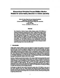
The Spike Sorting Task As outlined in the introduction, the term spike sorting is generally used to refer to the process of going from a raw, extracellularly recorded voltage trace to a representation of the signal in terms of spike times (i.e. the times when action potentials are observed) of individual neurons, the so called spike trains (as illustrated in figure 2.1).1 In this broad definition of term, spike sorting usually comprises several sub-tasks, such as preprocessing the raw data (e.g. high- or bandpass filtering), spike detection, i.e. the extraction of potential time points at which an action potential might have occurred, feature extraction, and the actual sorting stage. Sometimes a narrower definition of spike sorting is also used, which encompass only the actual sorting stage, excluding everything else. While the spike sorting algorithm introduced here will only deal with the actual sorting and will rely on previously developed methods for the preprocessing steps, it should be kept in mind that the performance of a spike sorting method (in the broad sense) crucially depends on the entire cascade of steps, not only on the sorting phase alone. In the following, the attention will mostly be restricted to the case where recordings are made using a single electrode, but the extension to the multi-electrode case is mostly straightforward (modulo some pre-processing). Almost all currently used spike sorting methods – including (to some extent) the GPUDPM spike sorting approach described in this report – operate according to the following scheme, which might be referred to as spike sorting by clustering and is illustrated in figure 2.2: First, potential action potential occurrence times are detected using some method for spike detection.2 In the simplest (but also 1

For a recent, general introduction to spike sorting see [Quiroga, 2007]; for background information on neural recording in the context of spike sorting see e.g. [Lewicki, 1998] or [Sahani, 1999]. 2 In the following, a distinction will be made between the terms action potential (AP) and spike: AP will refer to the true action potentials emitted by the neurons, whereas spike will be used to refer to the observed events in the recording that might correspond to true APs. The term occurrence time of an AP (or spike) will be used here to refer to the time at which the peak of the depolarizing phase occurs, and the term spike waveform refers to the recorded signal in some fixed interval surrounding a spike.

4

CHAPTER 2. SPIKE SORTING

5

2800

Neuron 1 1

2600

0.5

2400 0 5

votage

2200

→

2000 1800 1600

15

10 Neuron 3

15

10

15

0.5 0 5 1

1400 1200 0

10 Neuron 2

1

0.5

1

2

time

3

4

5

0 5

4

x 10

Figure 2.1: Schematic of the spike sorting task: The voltage trace from an extracellular recording is to be decomposed into the individual spike trains (occurance times of action potentials) of all neurons present in the recording.

most commonly used) form this is a simple threshold detector that marks all positions where the amplitude crosses a pre-determined threshold (which is usually set manually to some value relative to a multiple of the standard deviation of the signal). Several advancements over this simple method that operate more reliably under high noise conditions have also recently been proposed [Nenadic and Burdick, 2005; Choi et al., 2006; Rutishauser et al., 2006]. After spike detection, the segments surrounding spike occurrences are extracted using a fixed-size window of approximately the length of an AP (1–3ms, 20–60 samples at 20kHz). Each spike waveform can then be described by a vector containing the amplitudes of the signal at each of the sample points. Some form of dimensionality reduction or feature extraction is usually applied to the data set formed by these vectors, most prominently through principal components analysis (PCA) [Jolliffe, 2002] or noise-whitened PCA [Sahani, 1999]. Finally, some form of clustering is performed in this lower-dimensional or feature representation of the spikes.

2.1.1

Spike Sorting Challenges Numerous aspects make spike sorting a hard problem, the most important of which will be described here. Some of these difficulties have been dealt with by previous approaches to spike sorting; however the problem is far from being completely solved. Lewicki [1994] named three major problems for spike sorting: determining the AP shapes, determining the number of distinct shapes, and decomposing overlapping spikes into their component parts. Some progress on these issues has been made, but there are still problems that which have not been solved to satisfaction. Waveform non-stationarity, refractory period violations and an unknown number of neurons are problems that are addressed by the GPUDPM approach, and their significance will be explained below. The problem


6

100

Spike waveforms on EC Channel 1 300

200

50 100

0

0

−100

−50

−200

−300

−100 0

1

2

3

4

5

1

2

3

4

5

6

7

8

9

10

4

x 10

(a) Spike detection

(b) Spike extraction Projected Waveforms 5

4

4

3

3

2

2

1

1 PC 2

PC 2

Projected Waveforms 5

0

0

−1

−1

−2

−2

−3

−3

−4 −5 −10

−4 −5

0 PC 1

5

(c) Feature Extraction / PCA

10

−5 −10

−5

0 PC 1

5

10

(d) Clustering

Figure 2.2: Illustration of the stages employed by most current approaches to spike sorting. In order, these are: (a) spike detection, e.g. using some form of threshold detector as illustrated by the red line; (b) spike extraction by cutting a fixed-length window from the recording around the detected spike; (c) feature extraction, commonly done using principal components analysis (PCA); (d) spike clustering using some clustering technique.

of overlapping APs is also discussed, as this presents a major challenge that cannot be addressed within the current methodological framework. Waveform Non-Stationarity The fundamental assumption of spike sorting is that the action potentials generated by different neurons give rise to spike waveforms that have a characteristic shape, thus allowing them to be distinguished. While this assumption may generally be warranted, there is no reason to assume that the characteristic waveform stays fixed over time. As the characteristic waveform arises from several intrinsic and extrinsic parameters which can change over time, the waveforms will change


7

as well [Lewicki, 1998; Penev et al., 2001]. This phenomenon is referred to as waveform non-stationarity and constitutes a problem for most approaches to spike sorting. The changes in waveform shape can happen on several time scales: On a short time scale, waveform shape modulation can for example be due to repeated firing of the cell (bursting), leading to diminished signal strength in subsequent APs. While this process may be quite regular and thus amenable to direct modeling (as done e.g. by Sahani [1999]), there is also waveform change on a larger time scale due to extrinsic factors (e.g. electrode movement) and intrinsic factors (e.g. slow cell death or changes in the noise properties). As discussed below, many previous approaches have ignored waveform nonstationarity and have treated the characteristic waveform as fixed over time. While this may produce acceptable results when sorting short recordings, it breaks down when applied to long recordings lasting several days, such as those produced by implanted electrode arrays [Santhanam et al., 2007]. The GPUDPM approach allows the characteristic waveform of each neuron to change between spike observations and thus can account for waveform non-stationarity. Refractory Period Violations Right after a neuron fires an action potential it enters a state known as the (absolute) refractory period (RP), lasting for 2–3 ms, during which no further AP can occur. Thus, if a spike sorting algorithms assigns two spikes that occur within the RP of each other to the same source neuron, one knows that the assignment must be incorrect; such mistakes are known as refractory period violations (RPVs). While the number of refractory period violations occurring in a given assignment can be and is used as a diagnostic tool for assessing the quality of a given sorting [Harris et al., 2000], spike sorting algorithms should ultimately strive to make use of the information contained in the occurrence times of the spikes in order to obtain solutions that do not contain such violations. The timing information may even allow us to identify neurons that are otherwise indistinguishable, i.e. if the observed waveform shapes are almost identical. When combined with a probabilistic model that can provide an estimate of the uncertainty in each of the labels, inferences about the spiking behavior of these neurons can then still be made even if the spikes cannot be attributed to one neuron with certainty. The proposed spike sorting method explicitly models the absolute refractory period and provides a posterior distribution over labelings, thus automatically prohibiting solutions that contain RPVs and allowing inferences to be made even if the observed spike waveforms of two (or more) neurons are indistinguishable. The absolute refractory period is not the only characteristic of the intervals between successive APs from a single neuron (known as inter-spike intervals


8

or ISIs). The ISIs usually also follow a characteristic, heavy-tailed distribution (usually modelled as Exponential or log-Normal) whose parameter depends on the firing rate of the neuron. If the firing rate of the neurons remains relatively constant, the information contained in the ISIs can be exploited for spike sorting [Pouzat et al., 2004; Fee et al., 1996]. Unknown Number of Neurons In the settings where spike sorting is normally applied, the number of neurons whose spikes are present in a given recording is unknown a priori and thus has to be determined from the data. This is a common model selection problem, and standard model selection procedures (e.g. using the Bayesian information criterion (BIC), see [Burnham and Anderson, 2002]) can be applied. However, depending on the application, model selection may not be a feasible approach: As mentioned in the introduction, spike sorting can be a necessary preprocessing step for decoding in neural prosthetics. However, in order to make an algorithm suitable for this task it has to operate on-line.3 In an on-line setting where recordings are made over long periods of time, the number of neurons may vary over time, i.e. neurons can “appear” and “disappear” from the recording. As model selection is usually applied after a model has been fitted to the entire data set, they are unsuitable for the on-line applications. One could circumvent the problem by repeatedly refitting several models with different numbers of neurons as new data comes in and then applying model selection, but this may prove to be computationally too expensive or unreliable. Depending on the application for which spike sorting is used, it might also be desirable to obtain not only a single best assignment of spikes to some fixed number of neurons, but a whole distribution over assignments where the number of neurons stipulated is allowed to vary. The proposed spike sorting method sidesteps the model selection problem and provides a posterior distribution over clustering by employing a nonparametric Bayesian model. Such models have previously been successfully applied to the spike sorting problem [Wood et al., 2006; Görür, 2007; Wood and Black, 2008]. Overlapping Action Potentials Another problem is the possibility that more than one AP can be in progress at a given point in time. In this situation, the AP signals will mix in the recording and cause great difficulties for all approaches based on separate detection and clustering phases: When the APs occur at almost the same time, the resulting 3 Here on-line means that the algorithm operates on the data as it becomes available, i.e. the entire data set is not needed before the sorting process can begin.


9

signal will only contain one (larger) spike, and thus at least one AP will go unnoticed.4 If the APs occur not at the same time, but such that the resulting spikes lie within the spike waveform length of one another, it is possible to detect both spikes, but care must still be taken not to include the waveform of one spike within the other, as otherwise assigning it to the right source neuron will be very hard. Several practical approaches to the problem have been developed (see e.g. [Sahani, 1999] which introduces an additional spike detection phase after the model has been fitted). However, it seems a complete solution to this problem might only be possible by not separating the detection and clustering phases. The proposed method, as all methods which cluster spikes in some feature space rather than operating directly on the waveforms, cannot directly address the problem of overlapping APs. This aspect is a possible direction for further investigations, possibly based on an approach similar to that of Görür et al. [2004].

2.2

Previous Approaches The idea of recording extracellularly from multiple neurons and then grouping the actions potentials by source neuron is not new – it was first proposed in the 1960s [Gerstein and Clark, 1964] –, and since then numerous approaches to the problem have been developed. In the following a short outline of the development of spike sorting will be given, followed by a longer discussion of the approach of Wood and Black [2008] (of which the presented method is a direct extension) and the approaches of Bar-Hillel et al. [2006] and Wolf [2008] (which are direct competitors also addressing the problem of waveform non-stationarity).

2.2.1

Spike Sorting Through Clustering One of the simplest ways to group a given set of spike waveforms into clusters is by comparing them to a fixed set of template waveforms and then assigning them to the clusters whose template waveform they are most similar to (according to some measure of similarity). This is the approach taken by most early approaches to spike sorting (see [Schmidt, 1984] for a review), which mainly differ in the way the templates are constructed and how much intervention by a human operator is necessary. As distance measure, usually some form of squared error summed over all sample points was employed. However, it was soon realized that not all points in the sampled waveform are equally important for correct classification, which lead to the development of matching methods based on either 4

In practice, it is quite likely that both spikes will be lost or incorrectly assigned, as the signal resulting from the addition of the APs of two different neurons will be significantly different from each of the single signals.


10

hand-selected features such as peak or peak-to-peak amplitude, or automatically extracted features such as projections on the leading principal components. In the further development various clustering techniques were applied to such lowerdimensional representations of the spikes, which infer the templates automatically from the data in an unsupervised manner. Given a lower-dimensional representation of the spikes and disregarding the times at which the spikes occurred, the spike sorting problem reduces to a clustering problem, for which the statistics and machine learning communities have developed numerous algorithms (see e.g. [Duda et al., 2000]). It is thus not surprising that most of the better known clustering algorithms have been applied to spike sorting: k-means clustering [Salganicoff et al., 1988], hierarchical clustering [Fee et al., 1996], superparamagnetic clustering [Quiroga et al., 2004], as well as mixtures of Gaussians (MoG) [Sahani, 1999] and mixtures of t-distributions [Shoham et al., 2003]. Spike sorting algorithms based on Gaussian mixture models such as the one described in [Lewicki, 1998] and [Sahani, 1999] can be seen as the current defacto standard approach to the problem (apart from the still widely used manual “cluster cutting”), and many such algorithms are currently actively used on a daily basis in neuroscience labs. In the most basic version, these algorithms model the data as a mixture of K Gaussians, each of which has a mean µk and a covariance Σk , so that the probability of an observed (lower-dimensional representation of a) waveform x is given by P(x|θ1:K ) =

K X

N (x|µk , Σk )P(ck )

(2.1)

k=1

where θ1:K = {θ1 , . . . , θK } with θk = (µk , Σk ) are the parameters of all mixture components (in the following also referred to as component parameters) and P(ck ) are the mixture weights (corresponding to firing rates of the neurons).5 The means, covariances, and mixture weights in such a model can be efficiently learned using the expectation maximization (EM) algorithm [Dempster et al., 1977] or variants thereof [Sahani, 1999]. The algorithm of Sahani [1999] builds on such a simple model, but is greatly enhanced to allow the modeling of bursting behavior and overlapping spikes. One problem with this finite mixture Boldface symbols (µ, x, . . .) are used throughout this report to emphasize the fact that a variable is a vector. The individual components of such vectors are then referred to using non-bold symbols with subscript, e.g. x = (x1 , . . . , xD )T where the length should be clear from the context. However, in the later chapters this convention is sometimes dropped to keep the notation uncluttered, e.g. a (possibly multivariate) observation arriving at time t is simply denoted xt . The meaning should be clear from the context. MATLAB-style sequence notation is used to refer to sequences of variables, e.g. x1:T = x1 , x2 , . . . , xT . 5


11

model approach is that the number of clusters K is normally not known a priori (as discussed above). This problem can be addressed in numerous ways, e.g. by using model standard model selection techniques such as the Bayesian information criterion (BIC), through reversible jump Markov chain Monte Carlo methods [Nguyen et al., 2003], or by using a nonparametric Bayesian model as done in the approach of Wood and Black [2008] discussed next.

2.2.2

Nonparametric Bayesian Spike Sorting Building on previous spike sorting approaches based on Gaussian mixture models and the work of Rasmussen [2000], Wood and Black [2008] propose to use a Dirichlet process mixture of Gaussians model for spike clustering.6 The main advantages of using a such a model are (a) that the model selection problem can be sidestepped, and (b) that a full posterior distribution over possible labelings can be obtained, which can be used in further analyses and provides information about the confidence in a particular sorting. More specifically, Wood and Black [2008] use a Dirichlet process mixture of Gaussians model with a conjugate NormalInverse-Wishart prior, and employ a particle filter similar to that described by Fearnhead [2004], as well as an Markov chain Monte Carlo (MCMC) algorithm based on [Neal, 1998, Algorithm 3] for inference. The algorithm is shown to compare favorably to a finite mixture model on real neural data in terms of the log-likelihood of held-out data [Wood et al., 2006], but no comparison to previous approaches on data with known ground truth labeling was performed.

2.2.3

Sequences of Mixture Models The problem of waveform change over time, which is the main focus of the method developed in this report, has previously been addressed by other researchers. Bar-Hillel et al. [2005, 2006] propose a method for dealing with long-term non-stationarity by combining several Gaussian mixture models fitted to fixedlength time slices in a global model. According to the authors, the process used for combining the models across time is modelled after that used by human experts. Specifically, their approach operates as follows: First, the data is split into intervals of a pre-determined length, with enough data in each interval to fit a Gaussian mixture model. Several mixture models with different numbers of cluster and different initializations are then fitted within each time window. Afterwards, further mixture models are fitted by using the maximum likelihood (ML) solutions found in adjacent time windows as starting point, thus spreading 6

Dirichlet process mixture models will be discussed in more detail in section 3.2.


12

the local solutions to adjacent time frames. Finally, the optimal path through a global model of transition probabilities between MoG proposals – similar to a hidden Markov model (HMM) [Rabiner, 1989] and based on the Jensen-Shannon divergence – is found. The spreading process and the global optimization can be repeated to refine the solution. While this “dynamic Mixture of Gaussians” (dMoG) approach is shown to outperform other spike-sorting approaches (Learning Vector Quantization (LVQ), EM-based MoG, and superparamagnetic clustering) on synthetic non-stationary data sets, there are several drawbacks of this approach: First, because of the required global optimization, the algorithm cannot be used in on-line settings. Furthermore, the algorithm breaks down when waveform shape change occurs within one of the fixed-length windows, which have to be chosen large enough to ensure that sparse clusters are detected correctly. Finally, the algorithm only yields a single best solution rather than a posterior distribution over possible labelings. Wolf and Burdick [2007] propose a similar – but simpler – method for tracking neurons of changing waveform shape across fixed-length intervals.7 Their approach is also based on dividing the data into fixed-length time frames and then employing the EM algorithm to fit a mixture of Gaussians in each time frame. However, the models are not fitted independently but sequentially by using the means of the clusters found in the previous time steps as a prior for the cluster means in the current time step (the prior for each mean is a mixture of all means in the previous time step). Moreover, the results obtained in one time step are used to seed the EM algorithm in the next time step, while seeds for models with more or less clusters are created by a heuristic method. The number of neurons present in each time step is chosen by the Bayes information criterion (BIC), and neurons are associated across time steps by greedy matching. While this approach does not include a global optimization step and can thus be used in a (lagged) on-line setting, it suffers from the same problem of fixed-size time windows.

2.3

Preprocessing, Spike Detection and Feature Extraction As briefly mentioned before, preprocessing, spike detection and feature extraction are crucial ingredients for a robust and reliable clustering-based spike sorting algorithm. As the GPUDPM spike sorting algorithm described in this report requires as input lower-dimensional representations of extracted spike shapes, i.e. data to which this kind of preprocessing has already been applied, the 7

See also [Wolf, 2008] for a more comprehensive description of the procedure, including derivations.


13

most commonly used techniques will shortly be summarized here.8 Common preprocessing steps are reviewed in [Quiroga, 2007], on which the following summary is based. The first step after recording the data is usually to apply a high-pass (or band-pass) filter in order to remove components with frequencies that are not of interest; a passband of 300-3000Hz seems to be commonly used. Quiroga [2007] points out that non-causal filters should be preferred, as causal filters (such as IIR filters) might introduce problematic phase distortions. After filtering, the next step is spike detection, i.e. identifying potential occurrences of action potentials. As mentioned above, a rudimentary way of detecting spikes is to look for events that cross a fixed global threshold amplitude (either in the negative or positive direction, or both). The threshold can either be set manually (e.g. by inspection of plots such as the one shown in 2.2a where the threshold is indicated by the red line) or by using some fixed value relative to the standard deviation of the signal (values between 2σ to 5σ seem to be common). Choosing a good threshold is a difficult task and an incorrectly chosen threshold may have drastic effects: If chosen too low, the resulting data set will be noisy, and if chosen too high identifiable spikes could be missed. As reliable spike detection is a crucial link in the neural data analysis chain, more advanced methods that operate locally (e.g. using a sliding window threshold detector) instead of globally have been developed [Nenadic and Burdick, 2005; Choi et al., 2006; Rutishauser et al., 2006]. However, these will not be discussed in this thesis and the reader is referred to the mentioned papers. After detecting possible AP occurrences, the corresponding spike waveforms have to be extracted from the recording. This is usually done by cutting a fixedsize window of the length of an AP (between 1–3 ms) from the recording around the detected peak. The resulting slices, which (depending on the sample rate) are between 10 and 100 samples long, are the spikes that we want to sort. One step that is commonly applied between the extraction of the spikes and dimensionality reduction is re-aligning the spike waveforms at their minimum or maximum by first interpolating the spikes to a higher resolution, aligning them, and then downsampling them again. This reduces the variation in observed amplitude values merely due to the sampling points falling at slightly offset locations on the spike shape. This step becomes more important when low sample rates are used. If the recording electrode has more than one channel (so called tetrodes with four channels are commonly used), one way of combining the information from all channels is by concatenating the amplitude vectors before applying dimensionality reduction. To optimally leverage the information available through multiple 8

The procedures applied to the experimental data will be described in section 5.1.2.


14

electrodes more advanced methods are necessary. However, their discussion is again beyond the scope of this introduction. The final step before clustering is the extraction of discriminative features from the raw amplitude values. While the raw amplitude values could be used directly as input to the clustering algorithm, experiments have shown that spikes can be distinguished using only a relatively small number of features and that clustering in a lower-dimensional feature space is more robust to noise and also computationally attractive. In a comparison of different features for spike sorting Wheeler and Heetderks [1982] found that the features extracted through principal components analysis (PCA) [Jolliffe, 2002] can effectively be used to distinguish spikes in noisy recordings. Since then PCA has become the de-facto standard dimensionality reduction / feature extraction technique for spike sorting. An extension of PCA, which makes better use of the available information about the noise to determine discriminative features similar to linear discriminant analysis (LDA), called noise-whitened PCA (NwPCA) has also been proposed [Sahani, 1999] and is widely used. Figure 2.2 shows spikes extracted from the H ARRIS data set (see section 5.1.2) and their projection onto the first two principal components.

C HAPTER 3

Time-Varying Dirichlet Process Mixture Models This chapter will describe the time-varying Dirichlet process mixture model by first reviewing the Dirichlet process and its properties, then describing its applicability to mixture modeling, and finally reviewing several different approaches of introducing time dependence in such models. One such model, based on a generalized Pólya urn scheme, will be discussed in detail as it forms the basis for the spike sorting model described in chapter 4. Two sampling-based inference procedures – sequential Monte Carlo (SMC) and Markov chain Monte Carlo (MCMC) – for this model will be described in section 4.3 of the following chapter, including the spike sorting-specific modeling choices.1

3.1

The Dirichlet Process The Dirichlet process (DP) is a probability distribution over probability distributions, i.e. draws from the DP are themselves (discrete) probability distributions, allowing the DP to be used as a prior in nonparametric Bayesian models. More formally, the DP is a stochastic process whose sample paths are probability measures with probability one, and whose finite dimensional marginal distributions are Dirichlet distributed. The following overview is closely based on [Teh, 2007] which should be consulted for further details. Definition 1 (Dirichlet Process). Let G0 be a distribution over Θ and let α ∈ R+ . Further let A1 , . . . , Ar be a finite measurable partition of Θ. Then the vector (G(A1 ), . . . , G(Ar )) is random and distributed according to a Dirichlet process with base distribution G0 and concentration parameter α, written G ∼ DP(α, G0 ), if (G(A1 ), . . . , G(Ar )) ∼ Dir(αG0 (A1 ), . . . , αG0 (Ar )) for any finite measurable partition A1 , . . . , Ar of Θ. 1

See appendix B for a short introduction to sampling methods.

15

(3.1)

CHAPTER 3. TIME-VARYING DIRICHLET PROCESS MIXTURES

16

The existence of the Dirichlet process has been shown by Blackwell and MacQueen [1973] and in a more direct way, using a stick-breaking construction (see section 3.1.2), by Sethuraman [1994].

3.1.1

Properties of the DP The DP is an interesting mathematical object, but only its mathematical properties that are necessary for understanding the following discussion of DP mixture models will be considered here, namely the interpretation of its parameters G0 and α, as well as the posterior distribution of draws from a DP given some data. Parameters G0 and α The parameters G0 and α of a Dirichlet process DP(α, G0 ) can intuitively be understood as the mean and the precision of the DP respectively, because for G ∼ DP(α, G0 ) we have E [G(A)] = G0 (A) and V [G(A)] = G0 (A)(1 − G0 (A))/(α + 1). As α → ∞ we have G(A) → G0 (A) for any measurable A, i.e. G converges to G0 pointwise. Posterior Distribution As G ∼ DP(α, G0 ) we can draw samples θ1 , . . . , θN ∼ G and then consider the posterior distribution G|θ1 , . . . , θN . Let A1 , . . . , Ar be a finite measurable partition of Θ, and let nk be the number of observed values θi in Ak , i.e. nk = #{θi |θi ∈ Ak }. Then by the Dirichlet-Multinomial conjugacy we have (G(A1 ), . . . , G(Ar ))|θ1 , . . . , θN ∼ Dir(αG0 (A1 ) + n1 , . . . , αG0 (Ar ) + nr ) (3.2) which by definition 1 implies that the posterior distribution is a DP as well, with parameters given by ! PN δ α N i=1 θi G|θ1 , . . . , θN ∼ DP α + N, G0 + . (3.3) α+N α+N N In other words, the posterior is distributed according to a DP whose base distribution is a weighted average of P the prior base distribution G0 and the empirical distribution of the observations N i=1 δθi /N . The DP is thus a conjugate family that is closed under posterior updates.

3.1.2

Constructions of the DP The DP can be represented in different ways, and the representation to a large extent influences the inference procedures that can be developed. While many


17

inference schemes for DP mixture models are based on the stick-breaking construction, the time-varying Dirichlet process mixture model (DPM) that will be employed for spike sorting here is based on the Blackwell-MacQueen urn scheme / Chinese restaurant process (CRP) representation, thus both will be discussed in the following. Blackwell-MacQueen Urn Scheme The Blackwell-MacQueen urn scheme [Blackwell and MacQueen, 1973], also commonly referred to as the Pólya urn scheme, provides a way of constructing a sequence of draws θ1 , θ2 , . . . ∼ G with G ∼ DP(α, G0 ), without explicitly having to represent G. If we consider the posterior distribution of θn+1 |θ1 , . . . , θn with G marginalized out, it can be shown that ! n X 1 θn+1 |θ1 , . . . , θn ∼ αG0 + δθi (3.4) α+N i=1 and that marginally θ 1 ∼ G0 .

(3.5)

Together, (3.5) and (3.4) describe a sequential process of drawing θ1 , θ2 , . . . from G, which can be described by the following urn metaphor: First, draw θ1 ∼ G0 , paint a ball with that color and put it in the urn. Then, at each subsequent step n, either draw θn ∼ G0 with probability α/(α + n) and put a ball of that color in the urn, or, with probability n/(α + n), randomly draw a ball from the urn, set θn to its color, then paint a new ball in that color and return both balls to the urn. Clearly, under this process, some of the θi will be the same even if the underlying G0 is smooth. This is sometimes referred to as the clustering property of the DP, as the equivalence classes of θ1 , . . . , θn define a (random) partition of the set {1, . . . , n}. Thus, if φ1 , . . . , φm are the unique values among θ1 , . . . , θn , and ni is the number of times φi occurs among θ1 , . . . , θn , then we can rewrite (3.4) as ! m X 1 θn+1 |θ1 , . . . , θn ∼ αG0 + n i δφ i . (3.6) α+N i=1 Chinese Restaurant Process and Ewens Sampling Formula We can further tease apart the clustering property from the remaining structure of the DP by noting that the unique atoms are drawn independently from the base distribution φi ∼ G0 , and that one can generate a sample θ1 , . . . , θn by first generating the clustering structure in the form of a random partition A1 , . . . , Am of {1, . . . , n} (i.e. the Ai are disjoint non-empty subsets of 2{1,...,n} such that


18

Sm

Ai = {1, . . . , n}), then drawing φi ∼ G0 and finally setting θj = φi for i = 1, . . . , m and j ∈ Ai . The random, exchangeable partition of [n] = {1, . . . , n} generated by the clustering property of the DP is distributed according to what it known as the Chinese restaurant process (CRP) [Pitman, 2002, chapter 3] and has been studied independently of the DP under the name Ewens sampling formula [Tavaré and Ewens, 1997]. As this will form the basis of the model described in the next chapter, its properties will be discussed in more detail here. The Chinese restaurant process takes its name from a metaphor describing its construction: Imagine a Chinese restaurant which has an infinite number of tables, each of which can accommodate and infinite number of customers. As the first customer enters the restaurant, she chooses to sit at any table, which we will number 1. Now suppose n customers have already entered the restaurant and occupy tables 1, . . . , Kn . Denote by ci = k the fact that customer i sits at table k. Customer n + 1 chooses a table k to sit at according to the following probabilities:   PmKkn if k ∈ {1, . . . , Kn } P(cn+1 = k|c1 , . . . , cn ) = α+ αi=1 mi (3.7)  PKn if k = Kn + 1 α+ m i=1

i=1

i

where mk , (k = 1, . . . , Kn ) denotes the number of customers sitting at table k. In other words, given the seating arrangement of the previous customers, a new customer chooses to sit at an already occupied table with probability proportional to the number of customers already sitting at the table, and at a new table with probability proportional to the DP concentration parameter α. This process induces an exchangeable partition of [n] that is distributed according to the clustering property of the DP, i.e. the Blackwell-MacQueen urn scheme is recovered by independently drawing φk for k = 1, . . . , Kn . The Ewens Sampling Formula An alternative way of describing an exchangeable partition {A1 , . . . , Am } of [n] is by a vector of counts Cn = (C1 , . . . , Cn ), where Ci denotes the number of sets in {A1 , . . . , Am } that have size i, i.e. Ci = #{j|#Aj = i, j = 1, . . . , m}. Or, using the Chinese restaurant metaphor, Ci is the number of tables occupied by exactly i customers. The distribution of such a vector of counts that arises from the clustering property of a Dirichlet process with concentration parameter α is given by the Ewens sampling formula (ESF, also known as the Ewens multivariate distribution)


19

[Antoniak, 1974; Tavaré and Ewens, 1997]: n n! Y αaj P(Cn = an ) = α(n) j=1 j aj aj !

(3.8)

where α(n) = α(α + 1) · · · (α + n − 1), and an = (a1 , . . . , an ) are non-negative integers such that a1 + 2a2 + . . . + nan = n. The ESF has two interesting properties that will be exploited in the construction of a time-varying DPM in section 3.4: Firstly, the ESF defines a so called partition structure which means that if n customers induce a partition whose counts are distributed according to (3.8), then m < n customers that are randomly sampled (without replacement) will also have counts distributed according to (3.8) [Kingman, 1978, pp. 2–3]. In other words, randomly deleting customers (not considering at which table they are sitting) will result in a seating arrangement that is distributed according to the ESF. Secondly, if one customer (among n customers) is chosen at random and then all r customers sitting at the same table are deleted, then the partition induced by the remaining n − r customers is also distributed according to the ESF [Kingman, 1978, pp. 5–6]. This property is known as the species deletion property and is characteristic of the ESF [Tavaré and Ewens, 1997].2 Stick-Breaking Construction The stick-breaking construction of Sethuraman [1994] represents draws G ∼ DP(α, G0 ) as weighted sums of point masses. It is given by βk ∼ Beta(1, α) πk = β k

k−1 Y

(1 − βi )

i=1

φk ∼ G0 G=

∞ X

π k δφ k

(3.9)

k=1

The φk are referred to as locations and the πk as masses.3 The name “stickbreaking” comes from the fact that one can interpret the πi as the lengths broken off a unit length stick that is repeatedly broken in the ratio βi : (1 − βi ) as illustrated in figure 3.1.

3.2

Dirichlet Process Mixture Models One of the uses of the Dirichlet process is as mixing distribution in a mixture model, which in turn can be used for density estimation or clustering. 2

For other properties of the ESF, an overview of its development and applications as well as pointers to further references see the review by Tavaré and Ewens [1997]. 3 Some authors (e.g. Griffin and Steel [2006]) refer to βk as the masses.


20

π1

1 − β1 π2

(1 − β1 )(1 − β2 ) π3

(1 − β1 )(1 − β2 )(1 − β3 ) π4 π5 π6

Figure 3.1: Illustration of the stick-breaking construction for the Dirichlet process: πk are the lengthsQ of the pieces broken off from the length one stick by repeatedly breaking the remainder k−1 j=1 (1 − βj ) in the ratio (1 − βk ) : βk , where βk ∼ Beta(1, α).

Definition 2 (Dirichlet Process Mixture (DPM)). A Dirichlet process mixture (DPM) is a model of the following form xi |φi ∼ F (φi ) φi |G ∼ G G ∼ DP(α, G0 )

(3.10)

where the xi , (i = 1, . . . , N ) are observations that are modeled as exchangeable draws from a mixture of distributions F (φi ) and the mixing distribution G is drawn from a DP with base distribution G0 and concentration parameter α. Such a model is equivalent to the limit of the following finite mixture model with K components as K → ∞ [Neal, 1998; Rasmussen, 2000]: xi |ci , θci ci |p1 , . . . , pK θci p1 , . . . , p K

∼ F (θci ) ∼ Discrete(p1 , . . . , pk ) ∼ G0 ∼ Dir(α/K, . . . , α/K)

(3.11)

where ci ∈ 1, . . . , K is the class label of data point xi , θk , (k = 1, . . . , K) are the parameters associated with component k and pk are the mixing proportions on which a symmetric Dirichlet prior is placed. Various inference methods for such models exist: MCMC methods such as the ones reviewed in [Neal, 1998] have been shown to work quite well in practice, and have since then developed further [Jain and Neal, 2007]. SMC methods have also been explored [Quintana, 1998; MacEachern et al., 1999; Chen and Liu, 2000] and refined [Fearnhead, 2004].4 Recently a deterministic approximate 4

For a short introduction to sampling-based inference methods refer to appendix B.


21

inference scheme based on variational methods has also been proposed [Blei and Jordan, 2006]. Mixture models in general are a widely used tool for density estimation and clustering. However, finite mixture models (i.e. mixture models with a fixed, finite number of components K) can only be applied when the number of components is known a priori, or model selection procedures [Burnham and Anderson, 2002] have to be used to choose K. Infinite mixture models sidestep the model selection problem by in principle allowing an infinite number of components, only a finite number of which will have data associated with them. Thus, effectively the number of components K is inferred from the data, with a prior placed the expected clustering structure. Infinite mixture models thus have even wider applicability, as they can be used when the number of mixture components is not known a priori and model selection is not feasible (e.g. when on-line inference is required).

3.3

Dependent DPMs While DPMs are very flexible and powerful tools for modeling independent and identically-distributed (i.i.d.) data, they cannot directly be applied when data is not i.i.d., e.g. when there is some temporal or spatial structure associated with the data. In order to be able to model dependent data, it would be desirable to be able to construct a series of DPMs that are tied together by some covariate (e.g. time). Such models have recently been developed [Xing, 1995; MacEachern, 2000; Walker and Muliere, 2003; De Iorio et al., 2004; Gelfand et al., 2005; Srebro and Roweis, 2005; Zhu et al., 2005; Griffin and Steel, 2006; Caron, 2006; Caron et al., 2007; Ahmed and Xing, 2008; Ren et al., 2008] and can collectively be referred to as dependent Dirichlet process (DDP) models. Griffin and Steel [2006] give the following definition: Definition 3 (Dependent Dirichlet Process [Griffin and Steel, 2006, p. 3]). A dependent Dirichlet process is a stochastic process defined on the space of probability measures over a domain, indexed by time, space or a selection of other covariates in such a way that the marginal distribution at any point in the domain follows a Dirichlet process. Though not all of the above mentioned approaches explicitly construct such a stochastic process, this definition captures the idea behind all of them. Here we are mainly interested in the use of such processes to define what can be referred to as time-varying Dirichlet process mixture models (TVDPM). Such models can, among other things, be used for “evolutionary clustering” [Chakrabarti et al., 2006], i.e. clustering of data that has a temporal structure – such as spike data.


22

In the following paragraphs the approaches of MacEachern [2000], Griffin and Steel [2006], and Ahmed and Xing [2008] will briefly be discussed before turning to an in-depth description of the approach of Caron et al. [2007]. The first two are based on the stick-breaking representation of the DP while the remaining two are based on the CRP (cf. section 3.1.2). MacEachern [2000] introduced and rigorously defined the notion of the dependent Dirichlet process. His constructive definition is based on allowing the distribution of the stick lengths βk as well as the distribution of the atom locations φk (k = 1, 2, . . .) in the stick breaking construction (3.9) to change with a covariate x ∈ X. For a given index set X his construction introduces two stochastic processes ZX and UX which describe the influence of the covariate x ∈ X on the locations and stick lengths respectively. At a given level of the covariate, draws from these processes are then transformed such that their distribution is the base distribution G0 (which can also depend on the covariate) and the Beta(1, α) distribution respectively. MacEachern [2000] showed that such DDPs exist and that marginally for all x ∈ X draws from the DDP follow a Dirichlet process. Griffin and Steel [2006] use a similar approach, but instead of inducing dependence on a covariate x ∈ X by introducing stochastic processes from which βk and φk are obtained, they keep βk and φk fixed, but change the ordering in which the βk are combined into πk . More precisely, Y πk = βσi (x) (1 − βσj (x) ) (3.12) j≤i

where {σ(x)}x∈X is a stochastic process, draws from which are orderings of {1, 2, . . .}.5 Griffin and Steel [2006] describe how such ordering processes can be derived from point processes and derive results about the resulting correlation structure for the case of Poisson processes. They also give a Gibbs sampler inference scheme and describe applications in regression and volatility modeling. Ahmed and Xing [2008] describe a TVDPM specifically designed for the application of clustering data with temporal structure (and possibly known temporal dynamics). Their approach builds on [Xing, 1995] and operates by on the one hand tying together the CRP probabilities of consecutive time steps, and on the other hand allowing the cluster parameters to develop according to some Markovian dynamics from one time step to the next. In their time-dependent variant of the Chinese restaurant process – which they dub the recurrent Chinese restaurant process (RCRP) – customers are assumed arrive in fixed time epochs (e.g. days) t = 1, . . . , T . In the first epoch, the customers are seated according The definition of Griffin and Steel [2006] is more general with permutations of {1, 2, . . .} as a special case. 5


23

to the standard CRP (3.7). In all remaining epochs, however, the table sizes at the previous epoch are used to determine the “popularity” of a table. Specifically, the conditional probability of ct,i (the label of the i-th data point in epoch t) is defined to be ( (i) nk,t−1 + nk,t if k is an old cluster P(ct,i = k|ct−1,1:Kt−1 , ct,1:i−1 ) ∝ (3.13) α for a new cluster where nk,t−1 is the number of customers seated at table k in epoch t − 1, and (i) nk,t is the number of customers seated at table k in epoch t after observing the first i data points. The component parameters θk,t are carried over from t − 1 to t for all clusters that had data associated with them in epoch t − 1 by means of a Markovian transition kernel P(θk,t |θk,t−1 ), and parameters for new clusters are drawn from G0 . The authors derive this model in three different ways and give a Gibbs sampling procedure for performing inference; additionally, an extension for handling higher-order dependencies is presented. However, it is not directly obvious whether this model has an underlying DDP structure as defined above. The approach of [Caron et al., 2007] is in many respects very similar to this approach and will be described next.

3.4

Generalized Pólya Urn for TVDPMs Caron et al. [2007] describe a DDP mixture model where the covariates are discrete time steps t = 1, 2, . . . and which thus is also primarily aimed at the “evolutionary clustering” scenario. Intuitively, their approach is based on (a) extending the Chinese restaurant process to a time-varying process which they refer to as the generalized Pólya urn (GPU), and (b) tying together the component parameters θk at consecutive time steps through a transition kernel P(θk,t |θk,t−1 ).6 In order to achieve (a), the CRP prior distributions (3.7) are coupled together at consecutive time steps through a deletion procedure based on the partition structure and species deletion properties discussed in section 3.1.2. A general definition of the GPU mixture model, corresponding to the graphical model shown in figure 3.2 can be given as follows.7 For each time step 6

In the following, the mixture model based on the GPU scheme will thus simply be referred to as the GPU mixture model, GPU model, or GPUDPM for short. 7 For ease of presentation, the description is restricted to the case where exactly one observation xt occurs at each time step t. While the model described in [Caron et al., 2007] allows for multiple data points per time step, this added flexibility is not needed for spike sorting and would clutter the presentation with additional indices.


k = 1, . . . , Kt−1

k = 1, . . . , Kt

θk,t−1

θk,t

m ˜ k,t−2

m ˜ k,t−1

ct−1

ct

xt−1

xt

24

t = 1, . . . , T

Figure 3.2: Graphical model of the GPU time-varying Dirichlet process mixture model [Caron et al., 2007]. θk,t denotes the parameters of mixture component k at time step t, m ˜ k,t−1 denotes the number of customers sitting at table k after the deletion step at t − 1, and ct denotes the class label of data point xt . Furthermore, Kt refers to the number of mixture components that have had data associated with them within the first t time steps. While there in principle are an infinite number of mixture components, only a finite number will have data associated with them at any given t.

t = 1, . . . , T the generative process is: xt |ct , θct ,t ∼ F (θct ,t ) ct | m ˜ t−1 , α ∼ CRP(m ˜ t−1 , α) m ˜ t−1 |m ˜ t−2 , ct−1 ∼ DEL(m ˜ t−2 , ct−1 , ρ, γ) ( P(θk,t |θk,t−1 ) if k ∈ {1, . . . , Kt−1 } θk,t |θk,t−1 ∼ G0 if k = Kt−1 + 1

(3.14)

where xt is the observation at time t, ct is the associated label assigning the observation to a mixture component, and θk,t are the parameters of component k at time t. For notational convenience we can assume that the classes that have been created up to time t are labeled 1, 2, . . . , Kt−1 and that a new class created at time step t will always be labeled Kt−1 + 1. CRP(m ˜ t−1 , α) refers to the conditional probability of a class label ct given the seating arrangement after time

CHAPTER 3. TIME-VARYING DIRICHLET PROCESS MIXTURES step t − 1 denoted m ˜ t−1 = (m ˜ 1,t−1 , . . . , m ˜ Kt−1 ,t−1 ):  ˜k  Pm Kt−1 α+ i=1 m ˜i CRP(ct = k|m ˜ 1,t−1 , . . . , m ˜ Kt−1 ,t−1 , α) = α  PKt−1 α+

i=1

mi

25

if k ∈ {1, . . . , Kt−1 } if k = Kt−1 + 1

(3.15) This definition of the conditional label probabilities is similar to the CRP governing the conditional probabilities of the class labels in a DPM (3.7), with the difference being that here the table sizes m ˜ t−1 are not deterministically obtained from the remaining class labels, but rather evolve according to a specific deletion process, denoted DEL(m ˜ t−2 , ct−1 , ρ, γ), which will be described in the next section. Together, CRP and DEL constitute the GPU scheme: The Pólya urn scheme of Blackwell and MacQueen (cf. section 3.1.2) is extended to a time-varying process by re-using the same urn at consecutive time steps, while stochastically removing some balls between time steps. Caron et al. [2007] point out several features that distinguish the GPUDPM from other methods of constructing dependent Dirichlet process mixtures: Firstly, it operates in the representation of equivalence classes of cluster labels, i.e. the actual cluster labels do not matter but only their relative sizes, whereas in the stickbreaking representation employed by most other approaches the prior probability of a class label decreases with the label (e.g. class 1 has higher prior probability then class 2). The space of equivalence classes is to be preferred in clustering applications where the actual cluster labels are irrelevant and only the grouping of the data matters, or one has to ensure that the sampling procedure used for inference correctly mixes over the used labels [Jain and Neal, 2007]. Secondly, the proposed model marginally preserves the DPM model, i.e. marginally, at each time step, the data is modelled using a DPM. This is not clear for the other CRP-based models mentioned above.

3.4.1

Generalized Pólya Urn As outlined above, the generalized Pólya urn scheme augments the standard CRP with a deletion process DEL(·), thus making the CRP time-dependent. The deletion process DEL(m ˜ t |m ˜ t−1 , ct , ρ, γ) defines a scheme by which the number of customers sitting at each table in the Chinese restaurant develops over time and is defined as follows: Let mk,t denote the number of customers sitting at table k after seating all customers at time step t.8 In addition, let m ˜ k,t denote the same quantity after the deletion step at time t has taken place, and denote 8

Here, still, it will for ease of presentation be assumed that only one customer arrives per time step.


26

by mt and m ˜ t the vectors of both quantities for all components k = 1, . . . , Kt that have been created up to and including time t. The vector mt is obtained ˜ t−1 by adding in the customer arriving at time t, i.e. deterministically from m setting mct ,t = m ˜ ct ,t + 1. The generative process to obtain m ˜ t from mt can succinctly be described as: ( mt − ξ t with probability γ m ˜ t |mt , ρ, γ ∼ (3.16) mt − ζ t with probability 1 − γ where ξ t = (ξt,1 , . . . , ξt,Kt ), ξt,k ∼ Binomial(mk,t , ρ) and ζ t = (ζt,1 , . . . , ζt,Kt ), P t ζt,j = mt,j for j 6= ` and ζt,j = 0 for j = ` where ` ∼ Discrete(mt / K k=1 mk,t ). The entire GPU scheme can also be described in terms of an extended Chinese restaurant process metaphor: At time step t = 1 the first customer enters and sits at a table of her choice. At time step t > 1, t customers have entered the restaurant, nt of which are still in the restaurant (i.e. have not left yet) and occupy tables 1, . . . , Kt with mk,t , (k = 1, . . . , Kt ) customers sitting at table k. Before a new customer enters the restaurant at time step t + 1, customers randomly leave the restaurant according to one of the following two deletion procedures of which the first is chosen with probability γ and the second with probability 1 − γ, yielding updated table sizes m ˜ k,t : (1) Each customer currently sitting in the restaurant is independently considered for deletion with probability ρ, i.e. for each customer i = 1, . . . , t we draw ui ∼ Uniform(0, 1) and delete the customer if ui ≤ ρ. This is equivalent to sampling ∆mk,t ∼ Binomial(mk,t , ρ) and then setting m ˜ k,t = mk,t − ∆mk,t . (2) A customer is chosen at random and then all customers sitting at the same table are deleted. This is equivalent to sampling ! (m1,t , . . . , mKt ,t ) (3.17) ` ∼ Discrete PKt m k,t k=1 and then setting m ˜ `,t = 0 and m ˜ i,t = mi,t for all i 6= `. The first deletion procedure will be referred to as uniform deletion whereas the second will be called size-biased deletion. As noted in [Caron et al., 2007], both procedures ensure that the count vector corresponding to (m ˜ 1,t , . . . , m ˜ Kt ,t ) is distributed according to the ESF by the properties discussed in section 3.1.2. The new customer at t + 1 is then seated according to   Pm˜Kk,t if k ∈ {1, . . . , Kt } t m ˜ k,t P(ct+1 = k|m ˜ 1,t , . . . , m ˜ Kt ,t ) = α+ k=1 (3.18)  PKαt if k = Kt + 1 α+

k=1

m ˜ k,t

CHAPTER 3. TIME-VARYING DIRICHLET PROCESS MIXTURES and the table sizes m1,t+1 , . . . , mKt+1 ,t+1 are set to   ˜ k,t if k 6= ct+1 m mk,t+1 = m ˜ k,t + 1 if k = ct+1 ∧ ct+1 ≤ Kt   1 if k = ct+1 ∧ ct+1 = Kt + 1

27

(3.19)

where Kt+1 denotes the total number of tables that have been occupied up to and including time t + 1, i.e. either Kt+1 = Kt if the new customer has joined an already occupied table, or Kt+1 = Kt + 1 if the new customer sat at a new table. Note that the number of tables for which mk,t > 0 can be less than Kt ; such tables/clusters will be referred to as active or alive. Conversely, tables/clusters for which mk,t = 0 will be referred to as dead. Also note that new customers can only sit at active tables, as the probability of joining a table k with mk,t = 0 is zero. Thus, for practical purposes when doing inference only the active tables need to be kept track of. The GPU scheme can also be represented in an alternative way by introducing variables d1 , . . . , dt that denote the deletion times of customers 1, . . . , t.9 The cluster sizes (m ˜ 1,t , . . . , m ˜ Kt ,t ) can then be constructed from c1 , . . . , ct and d1 , . . . , dt as t X m ˜ k,t = I[ct0 = k ∧ dt0 > t] (3.20) t0 =1

where I[φ] is the indicator function that is 1 if φ is true and 0 otherwise and ∧ denotes the logical AND operator. If only uniform deletion is used, the “life span” of a customer arriving at time t, defined as lt = dt − t, has a geometric distribution (see section C.1) P(lt |ρ) = ρ(1 − ρ)lt

(3.21)

corresponding to the fact that the customer survived lt deletions and did not survive once. This alternate representation will be employed in the MCMC sampler that is described in section 4.3.2. A graphical model for this representation is shown in figure 4.4.

3.4.2

Transition Kernel P(θk,t |θk,t−1 ) The transition kernel P(θk,t |θk,t−1 ) ties together the cluster parameters across time steps, thus allowing them to vary from one time step to next. Thus, when applying the GPU model, the transition kernel P(θk,t |θk,t−1 ) should reflect one’s prior belief about how one expects the component parameters θk,t to change over 9

In the following the deletion times will also be referred to as the death times.


28

time. However, one is not completely free in choosing P(θk,t |θk,t−1 ): In order for the model to be marginally a DPM, the transition kernel P(θk,t |θk,t−1 ) must be chosen such that marginally ∀t θk,t ∼ G0 . In other words, G0 must be the invariant distribution of the Markov chain P(θk,t |θk,t−1 ), i.e. P(θk,t |θk,t−1 ) and G0 must satisfy Z G0 (θk,t−1 )P(θk,t |θk,t−1 )dθk,t−1 = G0 (θk,t ). (3.22) Given a base distribution G0 there are several methods for constructing P(θk,t |θk,t−1 ) such that (3.22) holds, two of which will be discussed in section 4.1.3.

C HAPTER 4

Spike Sorting Using Time-Varying DPMMs This chapter will describe in detail how the GPU model reviewed in section 3.4 can be instantiated and extended in order to be applicable to the spike sorting task. The specific modeling choices and options will be discussed and inference algorithms for the extended model will be given. Section 4.1 covers modeling choices, section 4.2 explains the modifications necessary in order to avoid refractory period violations, and section 4.3 gives SMC and MCMC inference algorithms.

4.1

Model As described in section 2.1, after preprocessing, spike detection and dimensionality reduction, we are left with D-dimensional representations of spike waveforms xi ∈ RD (i = 1, . . . , N ) that we wish to cluster. Additionally, each spike is associated with an occurrence time τi , and we assume that the spikes are ordered, so that ∀i < j : τi ≤ τj . The approach taken here is to model the xi as observations from a Generalized Pólya urn Dirichlet process mixture model (GPUDPM) such as the one described by (3.14). Each spike observation is thought to occur in its own time step t = 1, . . . , T , so that we can refer to the observations as xt (t = 1, . . . , T ).1 Each mixture component will correspond to one neuron, whose waveform shape is allowed to change over time. In order to fully specify the model in (3.14), the mixed distribution F (·), the base distribution G0 and the transition kernel P(θk,t |θk,t−1 ) have to be defined. To arrive at a convenient and computationally Note that the model utilizes two concepts of time: the discrete time steps t = 1, . . . , T , and the spike occurrence times τt . In the current version of the model the occurrence times τt are only used to order the spikes (i.e. to enforce ∀i < j : τi ≤ τj ) and to eliminate refractory period violations (see section 4.2), but are not otherwise included in the model. One consequence of this is that the amount by which the mean spike is expected to change between two successive observed spikes does not depend on the respective τt , but solely on the number of time steps elapsed between the occurrences (i.e. implicitly also on the firing rates of other neurons). This may not be desirable and is a possibility for further extensions (see section 6.1). 1

29

CHAPTER 4. SPIKE SORTING USING TIME-VARYING DPMMS

30

feasible model these components cannot be chosen independently, but the choice of the likelihood dictates suitable choices for G0 , which in turn restricts the possibilities for P(θk,t |θk,t−1 ). In the following, the likelihood model will be presented first, followed by a discussion of suitable choices for the corresponding G0 and P(θk,t |θk,t−1 ).

4.1.1

Likelihood / Waveform Shape Model The mixed distribution F (·) or – equivalently – the probability P(xt |ct = k, θk,t ) of a spike waveform xt given that we know it came from neuron k with parameters θk,t (in the following also referred to as the likelihood), defines how we expect observations from that neuron to “look” at that particular time. It is sensible to assume that the spikes generated by a neuron k at time t have some characteristic mean waveform µk,t , and that observed spikes from that neuron are corrupted by noise, i.e. xt = µk,t, + k,t where k,t is a zero-mean random variable.2 The term noise here covers all phenomena that are not explicitly modeled: true variation in the amplitudes of the action potentials emitted by the neuron (e.g. due to bursting), changes in the conductance properties of the tissue, overlap with APs from other, possibly distant neurons, as well as recording noise. We are thus interested in modeling the mean waveform as well as the characteristic variability around that mean waveform in the likelihood. Unfortunately, we are not completely free in choosing the likelihood, as it, together with the choices for G0 and P(θk,t |θk,t−1 ), largely determines the computational feasibility of the model. Here, the likelihood will be restricted to be Gaussian, though more flexible models (e.g. t-distributions, as suggested by Shoham et al. [2003]) could in principle be used if necessary.3 Thus in general we set P(xt |ct = k, θk,t ) = N (xt |µk,t , Λk,t ) (4.1) where θk,t = (µk,t , Λk,t ). If no restrictions are placed on the D × D matrices Λk,t this model can account for variability with arbitrary first-order correlations. As such a model can be (a) too flexible and (b) computationally inconvenient, restrictions can be placed on Λk,t , such as requiring it to be a multiple of the identity matrix Λk,t = λk,t I or a diagonal matrix Λk,t = diag(λ1,k,t , . . . , λD,k,t ) (this will be referred to as the diagonal model). Additionally, one could require 2

Here the term waveform is stretched to also refer to the representation of the waveform in feature space. 3 In the following the Gaussian/Normal distribution will be denoted by N , and will be parameterized by precision parameters λ (or Λ in the multivariate case) instead of the also often used parameterization in terms of variances σ 2 or covariance matrices Σ. The relation between the two is simply λ = σ −2 and Λ = Σ−1 . Generally, the parameterization of the distributions used follows [Bernardo and Smith, 2000, Appendix A].


31

the precision matrix to be the same for all components ∀k : Λk,t = Λt or fixed across time steps ∀t : Λk,t = Λk , or both. In the following, attention will mainly be restricted to the diagonal model but the full model will also be briefly discussed. While the diagonal model is mainly chosen for computational convenience, it is not necessarily true that the more flexible full model is the better choice in the context of the GPUDPM model. By allowing the mean waveform and covariance of each neuron to change from one time step to the next the model already is very flexible and can account for cluster shapes that are much more complex than the axis-aligned clusters of a simple MoG model with diagonal covariance matrix. As some of the observed correlations between features may be due to temporal effects (e.g. drifts of the recording electrode which may result in a decrease in amplitude and spike width) the diagonal model may be flexible enough to account for all the variation typically observed in neural data. To explore this is beyond the scope of this thesis, but could be a direction for further work. Diagonal Covariance Model The diagonal covariance model treats the noise in all dimensions as independent, i.e. the multivariate D-dimensional Gaussian with diagonal precision matrix is equivalent to the product of D univariate Gaussians: P(x|θ) =

D Y

N (xd |µd , λd )

(4.2)

d=1

where x = (x1 , . . . , xD ), θ = (µ1 , . . . , µD , λ1 , . . . , λD ) and the subscripts k and t have been dropped for notational convenience. In terms of waveforms, such a model entails the belief that the noise affects each dimension of the lower-dimensional waveform representation independently such that the resulting clusters are axis-aligned. While this assumption is not generally warranted for PCA projections of spike waveforms, it can serve as an adequate approximation in practice (for the reasons discussed above). For stationary mixture models this assumption is not normally made as estimation of the full covariance matrices can efficiently be performed using the EM algorithm. In the case of the GPUDPM model however, the diagonal model brings with it computational advantages that may outweigh the possibly small benefits of using a full covariance matrix.

4.1.2

Base Distribution G0 In DP mixture models, as well as in the GPUDPM model, the base distribution G0 acts as a prior over the parameters θ. It should thus reflect our prior belief of


32

how we expect the means and precisions of the individual clusters to vary. One computationally attractive and from a modeling perspective not unreasonable choice for G0 is the conjugate prior to the likelihood P(x|θ), i.e. in the case of the full model the Normal-Wishart Distribution given by G0 (µ, Λ) = N (µ|µ0 , κ0 Λ)Wish(Λ|ν0 , Λ0 )

(4.3)

and in the case of the diagonal model a product of independent Normal-Gamma distributions4 : G0 (µ1 , . . . , µD , λ1 , . . . , λD ) =

D Y

[N (µd |µ0 , n0 λd )Ga(λd |a, b)]

(4.4)

d=1

The R main advantage of this choice is that the predictive distribution P(x) = P(x|θ)G0 (θ)dθ and the posterior P(θ|x) are analytically tractable (see section C.2), which simplifies the inference procedures (see section 4.3). An obvious disadvantage of using the conjugate prior is coupling of the mean and the covariance in the prior, which may not directly reflect our prior beliefs about the variability of waveform shape. One could decouple the mean from the covariance at the cost of conjugacy by placing a Normal distribution on the mean and an Gamma/Wishart distribution on the covariance. For the diagonal model, another possibility would be choose a log-Normal instead of a Gamma prior on the variances. However, these extensions are not explored here as the conjugate prior has been shown to work well in practice [Wood and Black, 2008] and the expected benefits from using a non-conjugate prior are small.

4.1.3

Transition Kernels The transition kernel P(θk,t |θk,t−1 ) models the evolution of component parameters through time, i.e. in the spike sorting application it is used to model the prior belief about how the mean waveforms µk,t and noise precisions Λk,t are expected to change as time progresses form t − 1 to t. As discussed in section 3.4.2, the major restriction on the choice of P(θk,t |θk,t−1 ) is that it has to fulfill Z G0 (θk,t−1 )P(θk,t |θk,t−1 )dθk,t−1 = G0 (θk,t ). (4.5) However, there are some further properties that are desirable in terms of modeling and for computational reasons: Firstly, to simplify modeling it would be helpful to be able to control the amount of dependence between consecutive time steps We have chosen equal hyperparameters µ0 , n0 , a and b for all dimensions – this assumption could be relaxed if necessary. 4


33

though some parameter whose interpretation can easily be characterized. Secondly, for the sampling-based inference procedures described in section 4.3 to be applicable, one must be able to obtain samples from P(θk,t |θk,t−1 ). Furthermore, computational simplifications are possible if the posterior of the parameters given the parameters at the previous time step and the current data point xt P(θk,t |θk,t−1 , xt ) = R

P(θk,t |θk,t−1 )P(xt |θk,t ) P(θk,t |θk,t−1 )P(xt |θk,t )dθk,t

(4.6)

has a simple form and/or can easily be sampled from. In the following, two choices for P(θk,t |θk,t−1 ) will be discussed: one based on the update rule of the Metropolis algorithm, and another based on an auxiliary variable scheme. Both have advantages and disadvantages: The advantages of the Metropolis kernel are that it can be combined with any base distribution and likelihood and does not require additional auxiliary variables. The main drawback is that the dependence structure it introduces is not easily characterizable, and that one cannot sample from (4.6) directly. The auxiliary variable kernel removes both of these restrictions but requires a (possibly large) number of auxiliary variables and has to be re-derived for each choice of G0 . Metropolis Update Rule Kernel One possible choice for the transition kernel P(θk,t |θk,t−1 ) is the update rule used by the Metropolis algorithm [Metropolis et al., 1953]: P(θk,t |θk,t−1 ) = S(θk,t−1 , θk,t )A(θk,t−1 , θk,t ) Z 0 0 0 + 1 − S(θk,t−1 , θ )A(θk,t−1 , θ )dθ δθk,t−1 (θk,t ) where S(θk,t−1 , θk,t ) is a (symmetric) proposal distribution and G0 (θk,t ) A(θk,t−1 , θk,t ) = min 1, G0 (θk,t−1 )

(4.7)

(4.8)

is the probability of move.5 It can easily be shown that this transition kernel fulfills (4.5) (see e.g. [Neal, 1993, p. 55]). The general form of this transition kernel allows it to be used with arbitrary base distributions G0 as long as they can be evaluated. While sampling from this transition kernel is straightforward – a sample θ? from the proposal distribution is obtained and accepted with probability A(θk,t−1 , θ? ), or else is rejected in which case θk,t−1 is the new sample – evaluating the probability under this kernel can be difficult, as the integral may be analytically intractable. It may also be difficult to characterize the dependence structure induced by this update rule. 5

See section B.2.1 for a discussion of the Metropolis(-Hastings) algorithm.


ACF of µ

ACF

1.0

0.8

0.6

0.6

0.4

0.4

0.2

0.2

0.0

20

40

∆t

60

ACF of λ

1.0

0.8

80

100

0.0

34

0.01 0.1 0.2 0.5 1 5 10

20

40

∆t

60

80

100

Figure 4.1: Plot of the autocorrelation function for the mean (left) and precision (right) under the Metropolis transition kernel with Normal proposal distribution (determined empirically). The different lines show different values of the standard deviation of the proposal distribution. There parameters of G0 were a = 4, b = 1, n0 = 0.1, µ0 = 0. It can be seen that choosing the standard deviation too large (σ = 10) increases the autocorrelation again (due to rejections).

One possible (and popular) choice for the proposal distribution is an isotropic Gaussian centered at the old value S(θ0 , θk,t ) = N (θ0 |θk,t , σI).

(4.9)

The parameter σ controls the spread of the proposed jumps, and thus the dependence among consecutive time steps induced by the kernel: Small values for σ will lead to mostly small changes which will have a high probability of being accepted, thus leading to high correlations between consecutive time steps, while larger values will on the one hand lead to larger jumps thus decreasing correlations but on the other hand also lead to more rejections, thus increasing correlations. The effect of the parameter σ on the autocorrelation is shown in figure 4.1. Auxiliary Variable Transition Kernels Another possibility to construct a transition kernel P(θk,t |θk,t−1 ) with a given invariant distribution G0 is through the introduction of auxiliary variables zk,t,1:M = (zk,t,1 , . . . , zk,t,M ) (where each zk,t,m can be multivariate) that fulfill Z P(θk,t |θk,t−1 ) = P(θk,t |zk,t,1:M )P(zk,t,1:M |θk,t−1 )dzk,t,1:M (4.10)


35

zk;t;m k;t 1

m

= 1; : : : ; M

xt 1

k;t

xt

Figure 4.2: Schematic graphical model of the auxiliary variable transition kernel. The parameters θk,t for cluster k at time step t do not depend directly on the parameters from the previous time step, but through a set of M auxiliary variables zk,t,1 , . . . , zk,t,M . Also shown are the observations xt which depend on θk,t through the likelihood.

where P(zk,t,1:M |θk,t−1 ) and P(θk,t |zk,t,1:M ) are the conditionals of a joint distribution P(θ, z) (where θ denotes the parameters of any given cluster at any given time step, and z denotes the corresponding set of auxiliary variables) for which G0 (θ) is the marginal distribution of θ: P(θ, z) = P(z|θ)G0 (θ).

(4.11)

This is the approach of Pitt et al. [2002] and Pitt and Walker [2005] which is employed in the context of the GPU model by Caron [2006] (and possibly also in [Caron et al., 2007], where it is not explicitly mentioned). For a given G0 one has to specify P(z|θ) and then derive P(θ|z) = R

P(z|θ)G0 (θ) P(z|θ)G0 (θ)dθ

(4.12)

as well as (4.10). While this approach is valid (i.e. leads to the required invariant distribution) for any choice of P(z|θ), some choices will make computing (4.10) more tractable and/or simplify sampling from P(θ|z). One particularly convenient choice for P(z|θ) is the likelihood for which G0 (θ) is the conjugate prior, as in this case P(θ|z) will be of the same form as G0 (θ) and (4.6) can easily be sampled from. Pitt and Walker [2005] consider the case where the stationary distribution is a univariate Gaussian (in which case, if P(z|θ) is chosen to be Gaussian, the posterior and the transition kernel are also Gaussian) and the case where


ACF of µ

ACF

1.0

0.8

0.6

0.6

0.4

0.4

0.2

0.2

0.0

20

40

∆t

60

ACF of λ

1.0

0.8

80

100

0.0

36

M =1,ξ =1.00 M =10,ξ =1.00 M =100,ξ =1.00 M =1,ξ =0.10 M =100,ξ =0.10 M =1,ξ =10.00 M =100,ξ =10.00

20

40

∆t

60

80

100

Figure 4.3: Plot of the autocorrelation function for the mean (left) and precision (right) under the auxiliary variable transition kernel for the diagonal model with M auxiliary variables and a precision factor of ξ (with a = 4, b = 1, n0 = 0.1, µ0 = 0).

the stationary distribution is an Inverse-Gamma distribution. Building on this Caron [2006] derived auxiliary variable schemes for the case where the base distribution is a multivariate Normal distribution or a Normal-Inverse-Wishart distribution. In the following, an auxiliary variable scheme for the diagonal model with independent Normal-Gamma priors will be given, and the model derived by Caron [2006] for the Normal-Inverse-Wishart base distribution will be reviewed. Auxiliary Variable Transition Kernel for the Diagonal Model For the diagonal model, when we use the conjugate Normal-Gamma base distribution G0 (µ1 , . . . , µD , λ1 , . . . , λD ) =

D Y

[N (µd |µ0 , n0 λd )Ga(λd |a, b)]

(4.13)

d=1

we can easily derive an auxiliary variable kernel as described above by introducing M × D auxiliary variables zk,t,1,1 . . . . , zk,t,D,M (M for each of the D dimensions) with Normal conditional distributions zk,t,d,m |µk,t−1,d , λk,t−1,d ∼ N (µk,t−1,d , ξλk,t−1,d )

(4.14)

where ξ is an additional parameter that – together with the number of auxiliary variables M – controls the autocorrelation and variance of the transition kernel. Given the auxiliary variables, the conditional distribution of the parameters is


37

given by: µk,t,d , λk,t,d |zk,t,d,1 , . . . , zk,t,d,M ∼ N (µk,t,d |µM , nM λ)Ga(λk,t,d |aM , bM ) (4.15) where µM , nM , aM , bM are the updated parameters given by n0 µ0 + ξM z¯k,t,d nM ξM =a+ 2

µM =

nM = n0 + ξM

ξM s2k,t,d ξM n0 (¯ zz,k,d − µ0 )2 + 2 2nM P (4.16) M and z¯k,t,d is the mean of the auxiliary variables z¯k,t,d = m=1 zk,t,d,m /M and P s2k,t,d is the sample variance M s2kt,d, = M zk,t,d ). These formulas are m=1 (zk,t,d,m −¯ simply the posterior update formulas for the standard univariate Normal model for M observations with M replaced by ξM (see section C.2). The autocorrelation function (ACF) for this transition kernel for different choices of ξ and M is shown in figure 4.3. aM

bM = b +

Auxiliary Variable Transition Kernel for the Full Model The auxiliary variable transition kernel for the Normal-Inverse-Wishart (NiW) base distribution was derived by Caron [2006, pp. 125-125, 186-190] whose results will be summarized here. For a NiW base distribution G0 (µ, Σ|ψ) = NiW(µ, Σ|µ0 , κ0 , ν0 , Λ0 )

(4.17)

where ψ = (µ0 , κ0 , ν0 , Λ0 ) we can again define M (D-dimensional) auxiliary variables zk,t,1 , . . . , zk,t,M whose conditional distributions are Gaussian: zk,t,m |µk,t−1 , Σk,t−1 ∼ N (µk,t−1 , Σk,t−1 /ξ)

(m = 1, . . . , M )

(4.18)

where ξ ∈ ]0, ∞[ is a parameter controlling the amount of dependence.6 The posterior P(θk,t |z1,k,t , . . . , zn,k,t ) is then also a NiW-distribution with parameters given by the standard updating formula of the conjugate multivariate Normal model (see e.g. [Gelman et al., 2004, p. 87]): µk,t , Σk,t |zk,t,1 , . . . , zk,t,M ∼ NiW(µ00 , κ00 , ν00 , Λ00 ) 6

(4.19)

Note that here the parameterization of the Gaussian in terms of a covariance matrix rather than a precision matrix is used for convenience.


38

with κ0 ξM µ z¯k,t + κ0 + ξM κ0 + ξM 0 κ0 ξM Λ00 = Λ0 + (¯zk,t − µ0 )(¯zk,t − µ0 )T κ0 + ξM M X +ξ (zk,t,m − z¯k,t )(zk,t,m − z¯k,t )T

µ00 =

κ00 = κ0 + ξM ν00 = ν0 + M

(4.20)

m=1

4.2

Refractory Period Violations In addition to modeling waveform non-stationarity, the GPUDPM model can also be extended to avoid refractory period violations. Two main routes are possible to achieve this: The first is to explicitly model the ISI distribution with some parametric distribution (e.g. a shifted Exponential or a log-Normal distribution) and to include it in the likelihood part of the model. While this approach seems sensible and direct modeling of ISI density has been shown to improve spike sorting performance [Pouzat et al., 2004], how to do this in the framework of the GPUDPM model is not directly obvious and remains to be explored in future work. The route taken here is to make the whole model conditional on the spike occurrence times by modifying the conditional probability of assigning a spike to a cluster given the other cluster labels and the spike occurrence times τ1 , . . . , τt . For this, (3.7) is extended as follows:   if τt − τˆk,t ≤ rabs 0 P(ct = k|m ˜ 1:Kt−1 ,t−1 , c1:t−1 , τ1:t , α) ∝ m ˜ k if k ∈ {1, . . . , Kt−1 } (4.21)   α if k = Kt−1 + 1 where τˆk,t is the spike time of the last spike assigned to cluster k before time step t, i.e. τˆk,t = τt0 , t0 = max{t00 |t00 < t ∧ ct00 = k}. Essentially, what this means is that the conditional probability of assigning the spike at time t to cluster k is zero if the difference of the occurrence time of this spike and then occurrence time of the last spike associated with cluster k is smaller than the refractory period. In terms of the Chinese restaurant metaphor, this setup corresponds to a restaurant in which seating a customer at a table removes that table as an option for new customers for some period of time. This effectively incorporates the information contained in possible refractory period violations into the model while circumventing the explicit modeling of the ISI distribution. Note, however, that this introduces additional dependencies into the model: The occurrence time


39

of the last spike associated with cluster k before time step t, denoted τˆk,t , depends on the class labels of all data points since the birth of cluster k, thus, in the worst case it depends on all c1:t−1 . This, however, does not cause any difficulties with the inference algorithms presented next.7

4.3

Inference In this section the details of two inference procedures for the GPU spike sorting model will be given: a sequential Monte Carlo (SMC) algorithm – also commonly referred to as particle filter –, and a Metropolis-Hastings (M-H) sampler. The SMC algorithm in its general form was given by Caron et al. [2007] and some more details are specified in [Caron, 2006]. Here it is presented with the necessary details for the spike sorting application filled in. The Metropolis-Hastings sampler presented in section 4.3.2 is only loosely based on the Gibbs sampler outlined in [Caron et al., 2007].

4.3.1

Sequential Monte Carlo Algorithm 1 outlines a sequential Monte Carlo inference procedure for the sequence of target distributions πt (c1:t , Θ1:t , m ˜ 0:t−1 ) = πt−1 (c1:t−1 , Θ1:t−1 , m ˜ 0:t−2 ) × DEL(m ˜ t−1 |m ˜ t−2 , ct−1 ) × P(ct |m ˜ t−1 , Θt , c1:t−1 , xt , τ1:t ) ( Kt Y P(θk,t |θk,t−1 ) if k ≤ Kt−1 × G0 (θk,t ) if k > Kt−1 k=1

(4.22)

where Θt = (θ1,t , . . . , θKt ,t ) is the vector of parameters for all clusters at time t, and m ˜ t is the vector of cluster sizes after deletion at time t, i.e. the cluster sizes that will be used to determine P(ct+1 |m ˜ t , τ1:t+1 ) by (4.21), as t increases from 8 from 1 to T . This corresponds to the graphical model shown in figure 3.2 with the added dependence on τ1:t through (4.21). The presented algorithm follows the general sequential Monte Carlo scheme: At each time step t, the SMC algorithm first moves each particle forward in time 7

A further question of theoretical interest is whether this change results in a model that is still marginally a DPM, i.e. a DDP model according to definition 3. While I conjecture that this is not the case (certainly not when more than one data point is allowed to occur at each time step), this question is left as an open question for further research here, as it is not directly relevant for the application at hand. 8 See section B.3 for a short, general introduction to sequential Monte Carlo.


40

Algorithm 1 Sequential Monte Carlo for the GPU model [Caron et al., 2007] 1: for i = 1, . . . , N do (i) 2: w0 ← N1 3: end for 4: for t = 1, . . . , T do 5: for i = 1, . . . , N do 6: if t > 1 then (i) (i) (i) (i) 7: Sample m ˜ t−1 ∼ DEL(m ˜ t−1 |m ˜ t−2 , ct−1 ) . deletion step, eq. (3.16) 8: end if (i) (i) (i) (i) 9: Sample ct ∼ P(ct |m ˜ t−1 , Θt−1 , c1:t−1 , τ1:t , xt ) . sample label for xt , eq. (4.23) (i) 10: if ct = Kt−1 + 1 then (i) . xt assigned to new cluster, eq. (4.24) 11: Sample θ (i) ∼ q1 (θ|xt ) ,t ct (i) (i) 12: rnew ← G0 θ (i) /q1 θ (i) |xt . importance ratio for weight computation ct ,t

13:

else

14:

Sample θ

15:

rnew ←

16: 17: 18: 19: 20: 21: 22:

(i)

ct ,t

(i) ∼ q2 θ|xt , θ (i)

. xt assigned ct ,t−1 (i) (i) (i) P(θ (i) |θ (i) )/q2 (θ (i) |θ (i) , xt ) ct ,t ct ,t−1 ct ,t ct ,t−1 (i)

ct ,t (i)

to old cluster, eq. (4.26)

end if (i) for k = 1, . . . , Kt−1 such that m ˜ k,t−1 > 0 and k 6= ct do (i) (i) Sample θk,t ∼ P(θk,t |θk,t−1 ) . sample parameters from transition kernel end for (i) (i) (i) P(xt |θ (i) )P(ct |m ˜ t−1 ) ct ,t (i) (i) × rnew w ˜t ←wt−1 × (i) (i) (i) P(ct |m ˜ t−1 , Θt−1 , xt ) end for (i) (i) w ˜ w ˆt ← PN t (i) (i = 1, . . . , N ) . normalize weights

w ˜t (1) (N ) i1 , . . . , iN ; wt , . . . , wt i=i

(1)

(N )

23: ← R ESAMPLE[w ˆt , . . . , w ˆt ] 24: Create the new particle set by choosing the particles with indices i1 , . . . , iN 25: end for

by sampling a label for the data point xt (ll. 6–9) and new parameters for active all clusters (ll. 10–19) from suitable importance distributions, then computes the weight of each particle (l. 20) and finally selects a new particle set by resampling the current particles (ll. 22–24). Suitable choices for the resampling function R ESAMPLE[w1 , . . . , wN ] are discussed in section B.3.3. Algorithm 1 requires sampling from several distributions, each of which will be considered in detail in the following subsections. The distributions q1 (·) and q2 (·) denote generic importance distributions which, as discussed in section B.3.1, should approximate the true distribution as closely as possible.


41

Sampling from P(ct |m ˜ t−1 , Θt−1 , c1:t−1 , τ1:t , xt ) The label ct at time t can either be a currently active class (i.e. a class k for which m ˜ t−1,k > 0), or it can be a new class k ? . If we denote by Kt the number of classes created up to time t we can always choose k ? = Kt−1 + 1, thus conveniently labeling the classes 1, 2, . . . in the order in which they were created. For ct = 1, . . . , Kt the distribution P(ct |m ˜ t−1 , Θt−1 , c1:t−1 , τ1:t , xt ) is given by P(ct = k|m ˜ t−1 , Θt−1 , c1:t−1 , τ1:t , xt ) ∝ ( P(xt |θk,t−1 ) P(ct = k|m ˜ t−1 , c1:t−1 , τ1:t ) × R P(xt |θ)G0 (θ)dθ

if k ≤ Kt−1 if k = Kt−1 + 1 (4.23) where the first factor is given by (4.21). For any old cluster, the second term is simply the likelihood of xt given the cluster parameter θk,t−1 . As we have chosen the base distribution to be conjugate to the likelihood we can also analytically evaluate R the probability of the data point when integrating over the base distribution P(xt |θ)G0 (θ)dθ – this is a Student-t distribution (the required formulas for the diagonal model are given in section C.2). To sample from that distribution we can thus simply evaluate (4.23) for all possible choices of ct , normalize, and then sample from the resulting discrete distribution. Importance Distribution q1 (θk,t |xt , ct = k) The true distribution of the parameters θk,t for a new cluster given a newly associated data point xt is simply the posterior given by P(θk,t |xt , ct = k) = R

P(xt |θk,t )G0 (θk,t ) P(xt |θk,t )G0 (θk,t )dθk,t

(4.24)

which, again due to conjugacy, can be evaluated analytically, so we can set def

q1 (θk,t |xt , ct = k) = P(θk,t |xt , ct = k)

(4.25)

which is the optimal choice. The required formulas for the diagonal model are again given in section C.2. Importance Distribution q2 (θk,t |θk,t−1 , xt , ct = k) When new parameters are drawn for an existing cluster to which new data is associated, the distribution of the new parameters depends on the old parameters


42

(through the transition kernel) and the data point (through the likelihood). We have P(θk,t |θk,t−1 , xt , ct = k) = R

P(θk,t |θk,t−1 )P(xt |θk,t ) P(θk,t |θk,t−1 )P(xt |θk,t )dθk,t

(4.26)

When using the auxiliary variable transition kernel we can obtain a sample from this distribution by first sampling the auxiliary variables given the previous parameter from P(zk,t,m |θk,t−1 ), and then sampling the new parameters from the posterior P(θk,t |zk,t,1:M , xt ), which under our choice of distributions is a simple posterior update in the conjugate Normal model (again, see section C.2 for the required formulas in the diagonal model). For the Metropolis kernel however, it is not obvious how to sample from the distribution above. In this case we have to use an approximate importance distribution, and possible choices for q2 (·) are def

q2 (θk,t |θk,t−1 , xt , ct = k) = P(θk,t |θk,t−1 )

(4.27)

taking only the old parameters into account, or def

q2 (θk,t |θk,t−1 , xt , ct = k) = P(θk,t |xt , ct = k)

(4.28)

ignoring the old parameters but including the new data point; both choices are obviously sub-optimal. In the current implementation of the particle filter (4.27) is used for the Metropolis kernel.

4.3.2

MCMC Inference In the following, a Metropolis-Hastings sampler for the GPUDPM model will be described.9 While Caron et al. [2007] outline a Gibbs sampling procedure for the general GPUDPM model, their description is only schematic and it is not clear how to sample from some of the required posterior distributions in this instantiation of the model. Following Caron et al. [2007], the sampler operates in the alternate “deletion time” representation described in section 3.4.1: the state of the sampler consists of the allocation variables c1 , . . . , cT , their deletion times d1 , . . . , dT , and the cluster parameters for all active clusters, as well as the auxiliary variables for the random walk. Only the auxiliary variable kernel will be considered for use with the M-H sampler here, as the Metropolis kernel leads to further complications. Moreover, only uniform deletion will be considered. A graphical model for this representation of the model is shown in figure 4.4. 9

See section B.2.1 in the appendix for a short introduction to the Metropolis-Hastings algorithm.


43

zk;m;t m k

= 1; : : : ; M

= 1; : : : ; Kt 1

k;t 1 k

= 1; : : : ; Kt 1

k;t k

= 1; : : : ; Kt

dt 1

dt

ct 1

ct

xt 1

xt

t 1

t t = 1; : : : ; T

Figure 4.4: Schematic graphical model of the GPUDPM in the alternate representation ˜ t can using death times of allocation variables dt from which the occupancy counts m be reconstructed. Also shown are the auxiliary variables for the random walk zk,m,t and the occurrence times of the spike τt . Note that the allocation variables ct depend on all death times d1 , . . . , dt−1 and all previous allocation variables c1 , . . . , ct−1 , as well as all previous spike times τ1 , . . . , τt−1 .


44

In short, the sampler operates as follows: in each iteration all time steps t = 1, . . . , T are considered sequentially.10 At each time step, the allocation variable ct as well as the parameters for all active clusters at that time step are sampled from their respective posterior distribution. A M-H move is then employed to sample the deletion time dt , and another one for each active cluster to sample all auxiliary variables connecting t and t + 1 in the transition kernel. Each of these steps will be described in more detail in the following paragraphs. Initialization All variables in the state of the sampler have to be initialized to suitable initial values. The values stored in a particle from a run of the particle filter are a convenient starting point, but some additional values must be sampled: For the M-H sampler, cluster parameters (and corresponding auxiliary variables) must be present from time 1 until the death of the cluster in order to be able to compute the posterior distributions of the class labels which include the likelihood (see below). As the particle filter only starts to sample parameters for a cluster once a data point is assigned to it, the state has to be completed by sampling parameters for each cluster that is “alive” at any point from its “birth” backwards to time 1. The sampler could, of course, also be initialized in some other state, e.g. a state where all data points are assigned to one cluster and all parameters are initialized to the mean and variance of the data. However, the sampler might then need a large number of rounds to converge to the equilibrium distribution. Sampling the Allocation Variables ct A new value for the allocation variable ct at time step t can be sampled from its posterior distribution given the rest of the state, denoted P(ct |rest) where “rest” denotes everything in the state but ct . The possible values that ct can take on are the class labels of any cluster that is alive at time t or will be alive at some point t0 < dt (the set of these labels will be denoted Ktpossible ), or a currently unused label indicating that a new cluster is to be created (which will be denoted k ? ).11 As the posterior P(ct |rest) is proportional to the joint distribution, it can be evaluated by computing the joint for all possible values ct can take on and then normalizing the result. In this computation, only the parts which incorporate ct must be taken into account, so that for k ∈ Ktpossible ∪ {k ? } the posterior P(ct = k|rest) can be 10

The time steps could also be considered in a random order. All classes that are alive at any point are potential values for ct . However, for clusters that die before t or that are born after (or at) dt , the posterior probability for ct taking those values is zero. 11


45

computed as P(ct = k|rest) ∝

dt Y

˜ t0 −1 , τ1:t0 , c1:t0 −1 ) P(ct0 |m

t0 =t

( P(xt |θk,t ) × R P(xt |θ)G0 (θ)dθ

if k ∈ Ktpossible if k = k ?

(4.29)

where the conditional probability of the class label on the right hand side is ˜t defined as in (4.21) and is evaluated under the state in which ct = k (and the m are computed from the rest of the state using (3.20)). A new value for ct can then easily be sampled from the resulting discrete distribution. If ct takes on an entirely new label k ? (i.e. a new cluster is started) the state must further be amended by sampling parameters (and auxiliary variables) for that cluster for t0 = 1, . . . , dt . This can be done by first sampling θk? ,t from its posterior distribution given the data point at time t, and then sampling backward for t0 = t − 1, . . . , 1 as well as forward for t0 = t + 1, . . . , dt from the transition kernel. For computational reasons it is also sensible to store the current cluster birthand death times, as well as the time stamp of the last spike associated with each cluster at each time point. If ct takes on a new value, this additional information also has to be updated. Sampling the Cluster Parameters The cluster parameters θk,t for all clusters that are alive at time t (denoted k ∈ Ktalive ) can also be sampled from their posterior distribution given the rest of the state. The parameters θk,t only depend on the auxiliary variables from the previous times step (if any), the data point xt associated with it in this time step (if any), and the auxiliary variables leading to the next time step. Because of the conjugacy in the chosen distributions, the posterior distribution can be computed analytically. This can most easily be seen by viewing it as the posterior of a Normal likelihood and a Normal-Gamma prior: likelihood

prior

z }| {z }| { P(θk,t |rest) ∝ P(xt |θk,t )P(zk,1:M,t+1 |θk,t ) P(θk,t |zk,1:M,t ) = N (µk,t |µ0 , n0 λ0 )Ga(λk,t |a0 , b0 )

(4.30)

where µ0 , n0 , a0 , and b0 are the updated parameters for the Normal model when the auxiliary variables and (possibly) the data point xt are treated as observations (see section C.2 for the formulas).


46

Sampling the Auxiliary Variables The auxiliary variables zk,m,t that connect the cluster parameters at time step t − 1 to those at time step t are also part of the state of the sampler and have to be updated. As the posterior distribution P(zk,m,t |rest) ∝ P(zk,m,t |θk,t−1 )P(θk,t |zk,1:M,t )

(4.31)

does not allow to directly draw samples from it, a M-H update is performed for each active cluster k. The “forward” distribution P(zk,m,t |θk,t−1 ) is used as the jumping distribution to propose new values for all M auxiliary variables (denoted ? zk,1:M,t ), and the jump is then either accepted or rejected according to the standard M-H acceptance ratio (see (B.7) in section B.2.1) which in this particular case simplifies to p˜? (Ψ? )Jt (Ψt−1 |Ψ? ) p˜? (Ψt−1 )Jt (Ψ? |Ψt−1 ) ? ? P(zk,m,t |θk,t−1 )P(θk,t |zk,1:M,t )P(zk,m,t |θk,t−1 ) = ? P(zk,m,t |θk,t−1 )P(θk,t |zk,1:M,t )P(zk,m,t |θk,t−1 ) ? P(θk,t |zk,1:M,t ) = P(θk,t |zk,1:M,t )

r(Ψ? , Ψt ) =

(4.32)

where Ψ denotes the entire state of the sampler. Sampling the Deletion Times The deletion time dt could also be sampled from its posterior distribution in the same way as the allocation variable ct (i.e. by normalizing the relevant parts of the joint for all possible values that dt can take on). However, as there are usually a large number of possible values of dt to consider, this is computationally unattractive. A more convenient way of sampling a new value for dt is to again use a Metropolis-Hastings update: As jumping distribution to propose a new deletion time d?t the prior distribution of dt can be used, which we can directly sample from: lt? ∼ Geo(ρ) (4.33) d?t = t + 1 + lt? where Geo(ρ) denotes the geometric distribution (see section C.1) with ρ being the probability of deletion at each time step. Then, again, this new value is either accepted or rejected, according to the standard M-H acceptance ratio (see above). Again, the computation of the joint in the acceptance ratio can be restricted to the parts which include dt , i.e. the product of conditional probabilities of the class labels (as in (4.29)) (the prior probability of dt cancels with the proposal).

CHAPTER 4. SPIKE SORTING USING TIME-VARYING DPMMS Component

Parameter

Base distribution G0 E [µd ] = µ0 V [µd ] = b/(n0 (a − 1)) E [λd ] = ab−1 V [λd ] = ab−2

µ0 n0 a b

Transition Kernel Generalized Pólya Urn

M κ ρ α

47

Description The prior mean of the clusters. As the data is usually centered, this is usually set to 0. The scaling factor of the variance of the prior mean. Shape parameter of the gamma prior. Inverse scale parameter of the gamma prior. Number of auxiliary variables. Scaling factor of the variance. Probability of deletion. DP concentration parameter.

Table 4.1: Summary of the model parameters when using the diagonal likelihood model and the conjugate prior, as well as the auxiliary variable kernel.

4.4 4.4.1

Practical Considerations Choosing Parameters The GPUDPM spike sorting model is specified by three classes of parameters: the parameters of the base distribution G0 , the parameters of the transition kernel (i.e. the variances for the proposal distribution in the Metropolis transition kernel and the number of auxiliary variables and the variance scaling factor in the auxiliary variable transition kernel) and the parameters of the GPU scheme (α, the deletion probability ρ, and the mixing weight between uniform and size-biased deletion). The parameters for the diagonal likelihood model with conjugate prior and the auxiliary variable transition kernel are summarized in table 4.1. Both inference procedures also have parameters that need to be chosen: for the particle filter one needs to specify the number of particles and when and how to resample. For the MCMC algorithm one has to choose a number of burn-in iterations and the number of samples to collect. While all parameters have relatively clear interpretations by themselves, choosing “good” parameter values for a given data set is non-trivial. One practical way of choosing parameters for the base distribution is to repeatedly draw samples from it until the sampled values “look like” the observed data; The same approach can be applied to the parameters of the transition kernel as well.


4.4.2

48

Strength and Weaknesses of the Inference Procedures Both presented inference schemes have their strengths and weaknesses: the particle filter has the advantage that it can be used sequentially, i.e. predictions can be made as new data comes in. It also also comparatively efficient in terms of computation.12 However, there are also some drawbacks: firstly, sequential Monte Carlo methods are known to behave poorly in high dimensional settings, possibly leading to an inaccurate representation of the posterior distribution (in fact, the posterior estimate might collapse to a single point). If one is only interested in the MAP solution this is not overly problematic as one can then simply view the particle filter as a greedy method for finding the MAP solution. This, however, neutralizes one of the reasons for using a Bayesian spike sorting model, namely the ability to average further analyses over the posterior distribution. Secondly, as the particle filter only takes into account information from the past, it is likely to fail (i.e. represent the posterior inaccurately) when events in the future drastically influence the probability of events in the past unless very large numbers of particles are used. As an example, consider the case where two neurons produce spikes that are indistinguishable in the feature space (i.e. they would be modelled with Gaussians with the same mean and covariance). In this case, chances are that refractory period violations between those spikes will occur. The posterior distribution should reflect the facts that (a) there must be at least two neurons that produce spikes of this shape, and (b) all spikes of this shape could potentially have come from any of those neurons. However, the posterior estimate obtained using the particle filter might not reflect the true posterior correctly: If the first RPV occurs between first two spikes of this shape, the particle filter will assign the second spike to a new cluster, and all subsequent spikes will be assigned to either cluster (respecting potential further RPVs), thus it behaves as desired. However, if the first RPV occurs somewhere later in the recording (which is more likely), then there is very low probability of the spikes before the RPV being assigned to two distinct clusters, and this possibility will thus not be represented in the particle set. If we then encounter more and more RPVs with the first cluster, the probability of earlier and intermediate points also belonging to the other cluster grows, but the particle filter is unable to reflect this as it only proceeds forward (see the experimental results in section 5.3.2). 12

The current implementation in Python (see appendix D) is not particularly tuned for speed. A single step of the particle filter (including weight computation and resampling) with 1000 particles takes between 1 and 10 seconds (depending on the number of active clusters) on a 3GHz processor. However, it is not entirely unreasonable to assume that this could be sped up to real-time operation (i.e. around 100 spikes per second), especially as large parts of the algorithm can be parallelized.


49

The MCMC procedure does not suffer from this problem and can thus be used to “clean up” the particle filter output in such situations. In fact, as the MCMC algorithm needs to be initialized in some way (and the initialization may have a large impact on the number of iterations required to reach convergence), initializing the state with the output of the particle filter is a sensible approach to combining both methods. However, the major problem with the MCMC approach is its speed: because if the large number of dependencies in the model computing the required conditional and joint distributions is computationally expensive.13 For now, the use of the MCMC algorithm will thus be restricted to showing its advantage on the example described above (see section 5.3.2).

13

With the current implementation, the labels, death times, cluster parameters and auxiliary variables can be sampled with a rate of about 10 time steps per second on a 3GHz CPU.

C HAPTER 5

Experiments Experiments were performed on artificial and real spike data in order to evaluate the performance of the proposed spike sorting method in comparison with other approaches and in order to assess its behavior under various conditions. The main goals of these experiments are (a) to show that the proposed method compares favourably to existing methods on stationary and non-stationary data sets, and (b) to explore the behavior of the method under various conditions and parameter settings. The performed experiments can thus roughly be grouped into these two categories: quantitative comparisons on synthetic and real data are presented in sections 5.2.1 and 5.2.2 and exploratory experiments on synthetic data are described in section 5.3. Assessing the performance of a spike sorting algorithm and comparing it to other methods is – for several reasons – difficult. Firstly, in order to objectively evaluate the correctness of any grouping of the observed spikes by source neuron, one must have access to the true grouping, i.e. one must know which spikes originated from which neuron. For non-synthetic data this information cannot be obtained with current recording techniques. However, it is possible to record intracellularly from one neuron and extracellularly in the vicinity of this neuron, thus producing a partial ground truth labeling in which all spikes belonging to the neuron recorded from intracellularly can be identified [Harris et al., 2000]. Comparisons to labelings obtained by manual sorting are not very significant as these are known to vary strongly between human operators [Wood et al., 2004] and do not necessarily reflect the true labeling [Harris et al., 2000]. Secondly, even if the true clustering is known, a method for comparing the similarity between the true clustering and the inferred clustering (potentially with distinct numbers of clusters) is required. As the actual labels of the clusters are arbitrary, the comparison should solely be based on the partitioning of the data. While several similarity scores for clusterings have been proposed (see e.g. [Meila, 2003] for a recent review), these measures can be hard to interpret and do not always correspond to one’s intuitions. However, they are sufficient for comparisons between spike sorting algorithms, and thus two such scores will be used in the evaluation: the adjusted Rand index [Hubert and Arabie, 1985; Steinley, 2004] which attains its maximum value of 1 when the clusterings are equal and has an expected value of 0 for comparing random clusterings, and the 50

CHAPTER 5. EXPERIMENTS

51

variation of information (VI) proposed by Meila [2003] which ranges from 0 (equality) to 1 (absolute disagreement).1 Thirdly, it is hard to quantify the advantages that having access to a posterior distribution over clusterings provides without considering a specific application. Ultimately, comparisons should be made “end-to-end” for a specific application, i.e. including preprocessing, spike sorting and all further analyses. Such a comparison is beyond the scope of this thesis, however, and thus availability of the full posterior is only hinted at by providing results that are averaged over the posterior. While there is a large number of interesting experiments that could be performed to analyze and compare the presented model, the attention here is restricted to a relatively small subsets in order to keep the presentation clear: only diagonal Gaussian likelihood model is used, and only in conjunction with the auxiliary variable transition kernel. Furthermore, to reduce the computational burden, most experiments were only performed using the SMC algorithm, and the chosen data sets were kept rather short. If not specified otherwise, the parameters used in the experiments were: DP concentration parameter α = 0.1, probability of deletion ρ = 0.01, γ = 1 (i.e. only uniform and no size-biased deletion); Parameters of G0 (see figure 5.8c): µ0 = 0, n0 = 0.05, a = 3.7, b = 0.65. Residual resampling was used in the SMC algorithm, particle set was PN and 2the −1 only resampled if the effective sample size Neff = ( n=1 wn ) dropped below half of the number of particles used.

5.1 5.1.1

Data Sets Synthetic Data Sets Three synthetic data sets were created for the comparison of the different spike sorting methods, similar to those used by Bar-Hillel et al. [2006]. The first one (in the following denoted S YNTH -1 and shown in figure 5.1) contains no waveform shape drift and is intended as a simple baseline, while in the second one (denoted S YNTH -2, shown in figure 5.2) the clusters change their mean and covariance over time. The third one (shown in figure 5.5a) also contains waveform drift, but additionally includes neuron “birth” and “death” within the recording. The simulation procedure used for all synthetic data sets is as follows: Given the desired simulation length T (in ms) and, for each neuron k = 1, . . . , K, a mean firing rate λk (in Hz) as well as a mean and a covariance at the beginning and Here, as suggested in [Meila, 2003], the VI score is normalized by log2 N (where N is the number of data points) so that it ranges from 0 to 1 rather than from 0 to log2 N , as only comparisons on single data sets will be made, and this score is easier to grasp directly. 1


52

5

PC 2

PC 2

5

0

0

−5 5 5

0 −5 −5

0 PC 1

5

PC 1

4

−5 0

x 10 Time (ms)

Figure 5.1: Scatter plots of the S YNTH -1 data set ignoring time (left) and including time (right). The data set has been sub-sampled five-fold to aid visualization.

start end at the end of the simulation (denoted µstart and µend k , Σk k , Σk ), spike occurrence times τk,1 , τk,2 , . . . are first sampled according to

τk,t ∼ τk,t−1 + rabs + Exp(1000/(1000/λk − rabs )

(5.1)

until τk,t > T where rabs is the absolute refractory period set to 2 ms in all experiments, and τk,0 = 0. Then, for each τk,t an observation xk,t is sampled from a Normal distribution whose parameters are linearly interpolated between start and end: τˆk,t = τk,t /T µk,t = (1 − τˆk,t )µstart + τˆk,t µend k k Σk,t = (1 − τˆk,t )Σstart + τˆk,t Σend k k xk,t ∼ N (µk,t , Σk,t )

(5.2)

Finally, the occurrence times and observations from the individual neurons are merged to form a data set with T observations in which τ1 ≤ τ2 ≤ τT . All simulated data sets were two-dimensional; the actual parameters used for generating the synthetic data sets are given in section A. Data sets generated in this way are a (relatively crude) approximation to what one observes in real extracellular recordings. Note that, unlike in [Bar-Hillel et al., 2006], no noise is added to the data sets which makes them somewhat less realistic. However, the DPM and GPUDPM do not explicitly model noise


53

5

PC 2

PC 2

5

0

0

−5 5 5

0 −5 −5

0 PC 1

5

PC 1

4

−5 0

x 10 Time (ms)

Figure 5.2: Plot of the S YNTH -2 data set ignoring the time dimension (left) and including it (right). While the clusters overlap when time is not taken into account (left), they can easily be separated if time is incorporated (right).

events but operate under the assumption that every observed spike corresponds to an AP from some neuron and should be assigned to some cluster. While under ideal conditions this would be the right thing to do, problems during the spike detection stage and with overlapping APs render this assumption incorrect in current practical applications, which is why several other spike sorting algorithms include an additional cluster where noise events are collected. The GPUDPM approach could be extended in a similar way, though ultimately one should strive to solve the problems with spike detection and the decomposition of overlapping spikes. The reaction of the algorithm to noise will be discussed in section 5.3.2.

5.1.2

Real Data Set with Known Partial Ground Truth Labeling As previously mentioned, while it is not possible to obtain a full ground truth labeling for extracellular recordings, one can make simultaneous extracellular and intracellular recordings of a single cell, thus obtaining a partial labeling. This technique has been applied by Henze et al. [2000] and Harris et al. [2000], and the resulting data set has been made publicly available.2 The data set consists of simultaneous intracellular and extracellular recordings of cells in the 2

http://crcns.org/data-sets/hc/hc-1/


54

5

PC 2

PC 2

5

0

0

−5 5 0 −5 −5

0 PC 1

5

PC 1

−5 0

2 5 1 x 10 Time (ms)

Figure 5.3: Subsampled scatter plot of the first two principal components of the H ARRIS data set ignoring time (left) and across time (right). The red circles denote the spikes that were identified on the IC channel. It can be seen that the waveform of this neuron changes over time and in the end becomes indistinguishable from another neuron.

hippocampus of anesthetized rats. Recordings from an extracellular tetrode and an intracellular electrode were made simultaneously, such that the cell recorded on the intracellular electrode was also recorded extracellularly by the tetrode. Spikes detected on the intracellular (IC) channel are an almost certain indicator that the cell being recorded fired an action potential. Spikes detected on the extracellular (EC) channels may include the action potentials generated by the intracellularly recorded cell but almost certainly include spiking activity from other cells as well. The intracellular recording therefore can be used to obtain a ground truth labeling for the spikes originating from one neuron that can be used to evaluate the performance of human sorters and automatic spike sorting algorithms that sort extracellular recordings Harris et al. [2000]. However, by this method ground truth can only be determined for one of the neurons whose spikes are present in the extracellular recording, and this should be kept in mind when evaluating the performance of spike sorting algorithms on such a data set. Neither the correct number of distinct neurons recorded from by the extracellular electrode nor the correct labeling for any spikes not originating from the neuron recorded intracellularly can be determined by this methodology. The available data set consists of the raw waveforms (recorded at 10kHz) from several recordings sessions. A four-minute subset of the data was selected


55

and preprocessed in the following way: The data was bandpass filtered (300Hz – 3kHz), and spikes on the intracellular channel were detected as the local maxima of the first derivative of the signal larger than a manually chosen threshold. Spikes on the extracellular channels were determined as the local minima exceeding 4 standard deviations in magnitude. Spike waveforms of length 1 ms were extracted from around each spike (4 samples before and 5 samples after the peak). The positions of the minima within the spike waveforms were aligned by upsampling, shifting and then downsampling the waveforms. The extracellular spikes corresponding to action potentials from the identified neuron were determined as the spikes occurring within 0.1 ms of the IC spike. For each spike the signals from the four tetrode channels were combined into a vector of length 40. Each dimensions was scaled by the maximal variance among all dimensions and PCA dimensionality reduction was performed on the scaled data sets. The first three principal components were retained. The resulting data set (referred to as H ARRIS) consists of 3187 spikes, 831 originate from the identified neuron. As shown in figure 5.1, there is a clearly visible change in waveform shape of the identified neuron over time in this recording. Presumably this change in waveform shape is due to the slow death of the cell as a result of the damage done to the cell by the intracellular recording procedure.

5.2

Comparison with Previous Approaches The performance of the GPUDPM spike sorting algorithm was compared to two other state-of-the-art spike sorting algorithms: the DPM-based algorithm developed by Wood and Black [2008] (in the following simply referred to as “DPM”) and the algorithm described by Bar-Hillel et al. [2005, 2006] (in the following referred to as “dMoG” for “dynamic mixture of Gaussians”).3 A brief description of both algorithms was given in section 2.2.1. Both algorithms were run using their default parameter settings except where otherwise indicated.4 3

An implementation of the DPM spike sorting approach is available from http://www. gatsby.ucl.ac.uk/~fwood/code.html and an implementation of the dynamic mixture of Gaussians approach is available at http://aharon.barhillel.googlepages.com/ Spike_Sorting.zip. 4 The dMoG implementation, even though it does not include a prior over parameters, seems to have some dependency on the overall position and scale of the data. To circumvent problems that resulted from running the algorithm on the raw data sets, the data was shifted and scaled to match the mean and variance of a test data set provided with the implementation on which the algorithm works well. Furthermore, the provided implementation only operates on two-dimensional data, so that further dimensions had to be removed from the data sets for experiments with this algorithm (this only applies to the H ARRIS data set).


Algorithm GPUDPM DPM dMoG

MAP AVG MAP AVG Nslice = 100 Nslice = 500

S YNTH -1 VI Rand 0.001 0.999 0.001 0.999 0.000 1.000 0.000 1.000 X X X X

56 S YNTH -2 VI Rand 0.008 0.986 0.008 0.986 0.106 0.472 0.109 0.482 0.164 0.417 0.120 0.610

S YNTH -3 VI Rand 0.001 0.999 0.001 0.999 0.087 0.503 0.087 0.503 0.110 0.563 0.164 0.392

Table 5.1: Summary of the results on the two synthetic data sets: shown are the adjusted Rand index (Rand, range: 0=random to 1=correct) and the variation of information (VI, range: 0=correct to 1=maximally different) comparing the ground truth labeling to the clusterings returned by the algorithms. For the GPUDPM and the DPM the scores are shown for the MAP solution as well as averaged over the posterior distribution (AVG). The values marked with X could not be obtained because the available implementation failed on this data set, and boldface marks the best obtained results.

5.2.1

Performance on Synthetic Data The three algorithms were run on the three synthetic data sets using manually chosen parameters values. The base distribution for both DP-based algorithms was chosen to resemble the true distribution of the cluster parameters. As the dMoG algorithm does not include a prior over cluster parameters, the main parameters controlling the behavior of this algorithm are the length of the individual time slices Nslice and the range of considered number of clusters. Two different values for Nslice (100, 500) were compared, while the possible number of clusters was set to range between 2 and 6. The results are shown in table 5.1. As expected, the performance on the simple baseline data set S YNTH -1 is almost perfect for all algorithms. This mainly shows that although the GPUDPM model and inference algorithm are considerably more complex, it has comparable performance when applied to stationary data sets. The results on data set S YNTH -2 are more interesting: Here, as expected, the stationary DPM model fails as the clusters have considerable overlap when time is ignored. The dMoG model performs better, but, as can be seen, critically depends on choosing a good value for the window size Nslice . If the window size is chosen to big the clusters cannot be separated reliably, and if it chosen too small it becomes difficult to estimate the cluster parameters. The GPUDPM approach reliably tracks the clusters over time and only makes few mistakes on data points that lie between clusters. Plots of the resulting labelings are shown in figure 5.4. The fact that MAP and AVG values are (approximately) equal for the GPUDPM hints at the


57

5

PC 2

PC 2

5

0

−5 5

0

−5 5 5

0 PC 1

−5 0

PC 1

(a) Ground truth

4

−5 0

x 10 Time (ms)

(b) GPUDPM

5

PC 2

5

PC 2

5

0

4

x 10 Time (ms)

0

−5 5

0

−5 5 5

0 PC 1

4

−5 0

(c) DPM

x 10 Time (ms)

5

0 PC 1

4

−5 0

x 10 Time (ms)

(d) dMoG (Nslice = 500)

Figure 5.4: Results on the S YNTH -2 data set (subsampled). (a) shows the true labeling while (b) though (d) show the (MAP) labelings returned by the three algorithms. Note that the actual labels (i.e. plot symbols/colors) used are not relevant, but only the way the data is partitioned. For example, though different labels are used (a) and (b) correspond to almost identical clusterings.

fact that most particles in the particle set are very similar to the MAP particle. This can also be seen in some of the other experiments and is a problem with the SMC inference procedure: One possible explanation is that the number of particles is too small so that not many low-weight alternative solutions can be retained in the particle set. Using a (much) larger number of particles and/or a better resampling scheme [Fearnhead, 2004], or resorting to the M-H sampler are possible ways to alleviate this problem.


58

5 PC 2

(a)

PC 1

5 0 −5 0

2 4 Time(ms)

−5 0 4

x 10

0 −5 0

2 4 Time(ms)

4

x 10

PC 1

PC 2 2 4 Time(ms)

4

x 10

PC 2

PC 1

2 4 Time(ms)

x 10

2 4 Time(ms)

x 10

4

4

5

0 −5 0

x 10

0 −5 0

5

(d)

2 4 Time(ms)

4

5

0 −5 0

x 10

0 −5 0

5

(c)

2 4 Time(ms)

5 PC 2

PC 1

5

(b)

0

2 4 Time(ms)

0 −5 0

4

x 10

4

Figure 5.5: Results obtained on the S YNTH -3 data set using the three inference algorithms: (a) true labeling, (b) GPUDPM, (c) DPM, and (d) dMoG (Nslice = 500). The GPUDPM arrives at the correct labeling, while the DPM groups pairs of clusters together that overlap over time. The dMoG also has difficulties with this data set and does not combine all cluster correctly.


FP FN F -Score # RPV

GPUDPM MAP AVG 4.7% 4.7% 1.3% 1.3% 0.91 0.91 0 0

DPM MAP AVG 3.2% 2.6% 17.1% 22.2% 0.85 0.83 3 1.68

59 dMoG Nslice = 100 Nslice = 500 0.3% 7.2% 71.6% 1.6% 0.44 0.87 0 11

Table 5.2: Summary of the performance of the three algorithms on the H ARRIS data. Shown are the proportions of false positives (FP), false negatives (FN), and the F score F = 2×precision×recall precision+recall , as well as the number of refractory period violations (RPV) incurred by the solutions. The best results in each row are highlighted in boldface.

5.2.2

Performance on Real Data with Known Ground Truth Labeling The three algorithms were also compared on the H ARRIS data set in order to assess their comparative performance on real neural data. The results are summarized in table 5.2 and the obtained MAP labelings are shown in figure 5.6. The cluster corresponding to the intracellularly recorded cell was determined by identifying the cluster with the largest intersection with the true IC spikes. The GPUDPM approach outperforms both the DPM as well as the dMoG model on this data set which contains waveform drift. While the DPM achieves a smaller number of false negatives than the GPUDPM, it produces an unreasonably high number of false positives. The dMoG model performs better than the DPM when Nslice = 500 but fails for Nslice = 100; in both cases it is outperformed by the GPUDPM.

5.3

Exploration of Model Characteristics In order to explore the characteristics of the model and the behavior of the inference algorithms under various conditions, several additional experiments were conducted on synthetic data sets. Section 5.3.1 describes experiments were the model parameters were varied, whereas section 5.3.2 analyzes the performance of both inference algorithms on difficult data sets.

5.3.1

Sensitivity Analysis In order to assess the influence of the individual parameters and their interactions on the algorithm’s performance, a set of experiments was performed which varied the four most important parameters independently. The parameters that were varied were the hyperparameters of the base distribution G0 (effectively the prior for the cluster shape and location), the number of auxiliary variables used in


60

5

PC 2

PC 2

5

0

−5 5

0

−5 5 0 PC 1

−5 0

2 5 1 x 10 Time (ms)

0 PC 1

(a) Ground truth

(b) GPUDPM

5

PC 2

5

PC 2

−5 0

2 5 1 x 10 Time (ms)

0

−5 5

0

−5 5 0 PC 1

−5 0

(c) DPM

2 5 1 x 10 Time (ms)

0 PC 1

−5 0

2 5 1 x 10 Time (ms)

(d) dMoG (Nslice = 500)

Figure 5.6: Results on the H ARRIS data set (subsampled). (a) shows the true labeling while (b) though (d) show the (MAP) labelings returned by the three algorithms. The GPUDPM algorithm successfully tracks the waveform change over time, while the DPM model splits the data from the IC channel into two clusters.

the transition kernel (specifying how the waveform shape is expected to change over time), the deletion probability ρ and the DP concentration parameter α. Each parameter was varied in three discrete steps: The parameters used for the base distribution were a broad setting (α = 1.1, β = 0.5, n0 = 1), a narrow setting (α = 80, β = 4, n0 = 0.01), and an approximately correct setting (α = 3.7, β = 0.65, n0 = 0.05). Illustrative draws from the resulting prior distributions are shown in figure 5.8. The number of auxiliary variables (per time step and active cluster) were chosen to be M ∈ {1, 30, 100}, and α was

CHAPTER 5. EXPERIMENTS M

ρ

61

α=1

Narrow Prior α = 0.1

α = 0.01

α=1

Correct Prior α = 0.1

α = 0.01

α=1

Broad Prior α = 0.1

α = 0.01

1

0.1 0.015 0

X 0.14 (24.0) 0.19 (8.0)

0.20 (63.1) 0.14 (12.9) 0.20 (8.0)

0.23 (71.1) 0.22 (11.0) 0.10 (6.0)

X 0.33 (30.1) 0.37 (10.0

0.47 (40.1) 0.36 (9.0) 0.31 (4.0)

0.47 (35.1) 0.36 (4.0) 0.35 (5.0)

X 0.34 (14.5) 0.39 (10.0)

0.41 (18.1) 0.31 (6.0) 0.31 (3.0)

0.32 (7.6) 0.31 (5.0) 0.31 (3.0)

30

0.1 0.015 0

X 0.11 (48.2) 0.10 (19.0)

X 0.11 (30.6) 0.08 (14.0)

0.19 (92.7) X 0.07 (16.0)

0.15 (71.1) 0.01 (6.2) 0.02 (5.0)

0.10 (33.9) 0.01 (6.0) 0.01 (5.0)

0.09 (26.1) 0.01 (5.0) 0.01 (5.0)

0.29 (56.4) 0.17 (15.4) 0.17 (5.6)

0.32 (24.8) 0.19 (5.2) 0.15 (3.0)

0.21 (6.1) 0.20 (3.0) 0.17 (3.0)

100

0.1 0.015 0

X 0.14 (42.9) 0.09 (24.1)

X 0.08 (26.0) 0.09 (15.1)

0.22 (89.9) 0.09 (20.7) 0.08 (15.8)

0.15 (78.2) 0.01 (11.5) 0.04 (9.0)

0.08 (34.1) 0.01 (6.3) 0.02 (7.0)

0.06 (25.1) 0.01 (5.0) 0.01 (5.0)

0.20 (67.7) 0.11 (11.8) 0.17 (3.0)

0.17 (12.8) 0.18 (5.0) 0.17 (3.0)

0.18 (7.0) 0.14 (4.0) 0.16 (3.0)

Table 5.3: VI scores and average number of clusters (in parentheses) for the labelings obtained with the particle filter on the 81 tested parameter combinations. M denotes the number of auxiliary variables in the transition kernel, ρ is the probability of deletion and α is the DP concentration parameter. The Xs mark cases where particles with more than 100 clusters were created and the run was aborted (this is not a limitation of the algorithm but a constraint in place to save memory and processing time). The italiziced values correspond to the results shown figure 5.7, while boldface marks the best obtained results.

varied between α ∈ {0.01, 0.1, 1}. The deletion probability ρ was chosen from ρ ∈ {0.1, 0.015, 0} corresponding to mean survival times of about 9, 66, and an infinite number of time steps, respectively. The experiments were performed on the first 1000 data points of the S YNTH -2 data set, using the SMC algorithm with 1000 particles. All other parameters were kept fixed at the value described at the beginning of the chapter. The results are summarized in table 5.3 which shows the average VI score as well as the average number of clusters for each of the 81 possible parameter combinations. Four selected results are also shown in figure 5.7. Generally, the results reflect one’s expectations of the model’s behavior: if the prior is chosen too broad or too narrow, not enough or too many clusters are created. It is thus advisable to choose a prior that resembles the true distribution as closely as possible.5 If ρ is chosen too big, neurons that fire sparsely might incorrectly be split into several clusters over time, as the clusters may not survive until the arrival of the next observation. Choosing ρ too small is only problematic if the data set contains cluster death: a new neuron birth might be incorrectly assumed to be a continuation of an earlier cluster in this case. The number of auxiliary variables 5

While one obviously does not have access to the true distribution of the parameters underlying a given data set, one can repeatedly draw from the prior for various settings of the hyperparameters until the draws resemble the data set at hand. Whereas this is relatively straightforward for the DPM model (which suffers from the same problem), it is more difficult in the GPUDPM case as the draws should resemble the data at each time point, and not when pooled over time. However, one can still find sensible parameters by looking at several time slices of the data.


62 5 PC 2

(a)

PC 1

5 0 −5 0

5000 Time(ms)

−5 0

10000

0 −5 0

5000 Time(ms)

PC 1

PC 2 5000 Time(ms)

PC 1

PC 2 5000 Time(ms)

PC 2

PC 1

5000 Time(ms)

10000

5

0 −5 0

10000

0 −5 0

10000

5

(e)

5000 Time(ms)

5

0 −5 0

10000

0 −5 0

10000

5

(d)

5000 Time(ms)

5

0 −5 0

10000

0 −5 0

10000

5

(c)

5000 Time(ms)

5 PC 2

PC 1

5

(b)

0

5000 Time(ms)

10000

0 −5 0

5000 Time(ms)

10000

Figure 5.7: Selected results on the S YNTH -2 data set for four different extreme parameter settings. (a) show the true labeling; (b) shows a setting where the prior is chosen too broad, resulting in overlapping clusters; in (c) the prior is chosen too narrow such that some clusters are spilt into two; (d) shows a case where the deletion probability ρ is chosen too large, leading to problems with the sparse clusters; (e) shows a case where only one auxiliary variable is used, such that the cluster parameters can change dramatically over time.


63

4

4

4

2

2

2

0

0

0

2

2

2

4

4

4

4

2 0

2

4

4

2 0

2

4

4

2 0

2

4

4

2 0

2

4

4

2 0

2

4

(a) Broad prior (a = 1.1, b = 0.5, n0 = 1)

4

4

4

2

2

2

0

0

0

2

2

2

4

4

4

4

2 0

2

4

4

2 0

2

4

(b) Narrow prior (a = 80, b = 4, n0 = 0.01)

4

4

4

2

2

2

0

0

0

2

2

2

4

4

4

4

2 0

2

4

4

2 0

2

4

(c) Approximately correct prior (a = 3.7, b = 0.65, n0 = 0.05)

Figure 5.8: Draws from the prior for the three parameter settings used in the sensitivity analysis. Each of the nine plots shows the isocontours of five draws from the base distribution G0 as well as draws from the Normal distribution with these parameters.


64

5

PC 2

PC 2

5

0

−5 5

0

−5 5 5

0 PC 1

4

−5 0

x 10 Time (ms)

(a) 2% noise

5

0 PC 1

4

−5 0

x 10 Time (ms)

(b) 10% noise

Figure 5.9: Comparison of the clusterings obtained with the GPUDPM model on the S YNTH -2 data set in the presence of 2% (a) and 10% (b) uniform noise.

controls how much the cluster parameters can change from one time step to the next, and thus choosing it too small results in clusters changing locations too quickly. One would expect that if the number of auxiliary variables is chosen too large the algorithm will not track waveforms that change quickly but rather assign the different waveforms to a new cluster. However, with 100 auxiliary variables this effect cannot be seen. The DP concentration parameter α controls the model’s “willingness” to assign data points to new clusters, and thus in the results a trend can be seen of lower values of α leading to a smaller average number of clusters. However, the influence of this parameter does seem rather weak relative to the other ones.

5.3.2

Failure Modes and Problematic Cases Noisy Data In its current version the GPUDPM model does not explicitly model noise events, i.e. spikes that should not be treated as belonging to any neuron because they are more likely artifacts of the employed preprocessing procedures. In other mixtures of Gaussians spike sorting models this is usually handled by including a very broad cluster with low weight in the model, to which all spikes that do not fit into any of the other clusters are assigned. In order to assess the behavior of the model and the SMC inference algorithm in the presence of noise, the particle filter (using the parameters described in section 5.2.1) was run on the S YNTH -2 data set after 2% and 10% uniform noise in the range [−5, 5] were added to the


65

data set. The results are shown in figure 5.9. In the presence of 2% noise the algorithm still correctly tracks all clusters over time and the noise events that do not overlap with the true waveforms (or have refractory period violations with these) are grouped into several other clusters (avg. VI: 0.025, avg. number of clusters: 40). This is the expected and – under the assumption that there are no true noise events – desired behavior: Spikes that are too different from other spikes simply start new clusters as they must belong to other neurons. With 10% noise the algorithm is still able to track three of the clusters correctly but splits the remaining two clusters into four across time (avg. VI: 0.121, avg. number of clusters: 108). This behavior seems to be fairly typical in the presence of noise, as it could also be observed on several other real data sets. This is likely to due noise events that are similar to the clusters’ waveform shape causing refractory period violations. While the algorithm still works fairly well under these noise conditions, an explicit model for such noise events should be included in the model if one expects there to be true noise events (e.g. due to imperfect preprocessing) in the data. Crossing Trajectories One of the few scenarios that is problematic for the model (or, more correctly, for the employed inference algorithms) is one where the waveform shapes of two neurons “drift across” each other, i.e. they drift in such a way that the become indistinguishable for a short period and then become distinguishable again. An illustrative example of this scenario is shown in figure 5.10. In terms of the model, the posterior distribution in this scenario should not only reflect the uncertainty for the short time when the waveforms are indistinguishable, but should also reflect both possibilities that the shapes either “deflected” (this is the MAP solution obtained using the particle filter) or “crossed” (the true labeling in this case), and both should be approximately equiprobable. However, the SMC algorithm as well as the M-H sampler fail to recover this posterior correctly: When the particle filter is applied to the shown data set, its posterior distribution mostly collapses to a single point, and the only solution that is represented is the one shown. The M-H sampler, when initialized with the MAP particle solution, mixes over the labels in the overlap area, but does not mix over the two scenarios. This can be seen from the bottom panel of figure 5.10, which shows a plot of the label entropy at each time point.6 The entropy before and after the overlap area is mostly zero, i.e. those labels are fixed at one value and do not change. Before computing the entropy the labels were mapped to 0, 1, . . . in the order in which they appeared in the labeling, thus mapping them to the space of partitions. 6


66 5

PC 2

(a)

PC 1

5

0

−5 0

2 4 Time(ms)

0

−5 0

6 4

x 10

0

Entropy

−5 0

1.0 0.8 0.6 0.4 0.2 0.0

Entropy

(c) 1.0 0.8 0.6 0.4 0.2 0.0

x 10

2 4 Time(ms)

x 10

4

5

PC 2

(b)

PC 1

5

2 4 Time(ms)

2 4 Time(ms)

6

0

−5 0

4

x 10

Label Entropy (M-H sampler)

0

0

4

10000

20000

30000

40000

50000

60000

10000

20000

30000 Time (ms)

40000

50000

60000

Average Label Filtering Distribution Entropy (SMC)

Figure 5.10: Results on a synthetic data set where the waveform shape of two neurons changes in such a way that their trajectories cross at some point in time (i.e. they become indistinguishable for a short period). The true labeling is shown in (a) and the MAP labeling returned by the particle filter in (b). In the MAP labeling the labels are switched after the clusters become indistinguishable. The correct solution is neither represented in the particle set, nor does the M-H sampler sampler mix to it within 5000 sweeps. Panel (c) shows the entropy of the label distribution at each time step computed from the samples obtained from the M-H sampler (top), and the average entropy of the label filtering distribution obtained from the particle filter (bottom). Note that the bottom of (c) shows the entropy of the filtering distribution within a single particle averaged over the entire particle set – the entropy for the labels represented in the final particle set is 0 for almost all labels. The samples obtained from the M-H sampler in 5000 iterations do not reflect the true uncertainty in the labels for the period after the indistinguishable phase.


2

4 6 Time step

8

10 0.0 0.1 0.2 0.3 0.4 0.5 0.6 0.7 0.8 p(labeling)

0

2

4 6 Time step

8

4 6 Time step

8

Labelings

(d) 0

2

Prior probability

Labeling

Labelings

Prior probability

Labeling

(b) 0

(c)

Labelings

10 0.00 0.05 0.10 0.15 0.20 0.25 0.30 0.35 p(labeling)

10 0.00

0.02

0.04 0.06 p(labeling)

0.08

0.10

Prior probability

Labeling

(a)

Prior probability

Labeling

Labelings

67

0

2

4 6 Time step

8

10 0.0 0.1 0.2 0.3 0.4 0.5 0.6 0.7 0.8 p(labeling)

Figure 5.11: Prior probability for the ten most probable labelings in each of the four conditions (for α = 0.1 and ρ = 0): (a) no RPV, (b) RPV between 1 and 2, (c) RPV between 4 and 5, and (d) RPV between 9 and 10. The color of the squares (black or white) indicates to which cluster a point belongs. For example, the first row in (a) corresponds to the clustering where all points are assigned to one cluster, whereas the second line in (b) means that the first point is a singleton, and all other points are assigned to a second cluster. The right panels show the prior probability of the labelings. The grid lines are only visual aids and carry no further meaning.

Refractory Period Violation Occurrence Another interesting issue to investigate is the influence of the occurrence time of the first RPV between two clusters on the model and the inference algorithms. To illustrate this, consider the following scenario: Two given neurons produce spikes of exactly the same shape, and thus are indistinguishable in terms of shape. However, there are refractory period violations between the two, so that the algorithm cannot group them in the same cluster. The question now is in how far the position at which the first first RPV occurs influences the posterior distribution over labels, both in terms of the true distribution and in terms of the approximations obtained using the inference algorithms. An experiment was conducted on the following illustrative data set: Ten spikes, each with waveform shape [0, 0]T , were placed 3ms apart (thus incurring no RPVs). Three variations of this data set were then made: In the first there is a RPV between the first and the second data point, in the second there is one between the fourth and the fifth, and in the third the RPV occurs between the 9th and the last data point. Also, for tractability, it was assumed that the death times of all labels lie beyond the end of the data set. The DP concentration parameter α was set to α = 0.1. Under these conditions the joint prior distribution over the 115,975 possible

(c)

Entropy

(b)

Entropy

(a)

Entropy

CHAPTER 5. EXPERIMENTS 1.0 0.8 0.6 0.4 0.2 0.0

1.0 0.8 0.6 0.4 0.2 0.0

1.0 0.8 0.6 0.4 0.2 0.0

0 5 10 15 20 25 Time

0 5 10 15 20 25 Time

0 5 10 15 20 25 Time

68

1.2 1.0 0.8 0.6 0.4 0.2 0.0 0 5 10 15 20 25 Time

1.0 0.8 0.6 0.4 0.2 0.0

1.0 0.8 0.6 0.4 0.2 0.0

1.0 0.8 0.6 0.4 0.2 0.0

1.0 0.8 0.6 0.4 0.2 0.0

0 5 10 15 20 25 Time

0 5 10 15 20 25 Time

1.0 0.8 0.6 0.4 0.2 0.0

0 5 10 15 20 25 Time

0 5 10 15 20 25 Time

0 5 10 15 20 25 Time

1.0 0.8 0.6 0.4 0.2 0.0

1.0 0.8 0.6 0.4 0.2 0.0

1.0 0.8 0.6 0.4 0.2 0.0

0 5 10 15 20 25 Time

0 5 10 15 20 25 Time

0 5 10 15 20 25 Time

Figure 5.12: Entropy of the marginal distribution of each individual label under the following four conditions (from left to right):no RPV, RPV between 1 and 2, RPV between 4 and 5, and RPV between 9 and 10. (a) shows the entropy under the prior, (b) the approximation by the M-H sampler, and (c) the approximation using the SMC algorithm.

clusterings (i.e. the product of the modified CRP probabilities in (4.21)) can be computed analytically and can be used as proxy for the posterior distribution as the contributions from the likelihood can be neglected (they are the same for all data points). Figure 5.11 shows the ten most probable clusterings under the prior (with α = 0.1 and ρ = 0) for each of the four conditions. Note that some results are somewhat counterintuitive. For example, the clustering with the highest probability in 5.11d is about 85 times more probable than the second one, though intuitively one might suspect that they should be about equiprobable. To assess how accurately the two inference procedures recover the posterior distribution, the particle filter (using 5000 particles) was then run on this data set, and an additional 2000 samples were obtained with the M-H sampler (initialized with the MAP particle) for each data set. Table 5.4 shows the KL divergence between the estimated distributions over clusterings to the true distribution under the prior. As expected, the approximation using the SMC algorithm becomes

CHAPTER 5. EXPERIMENTS Table 5.4: Kullback-Leibler divergence between the approximate distribution represented by the samples obtained from the particle filter or the M-H sampler, and the true distribution of the labelings under the prior.

69 Condition no RPV RPV 1-2 RPV 4-5 RPV 9-10

SMC 0.390 0.870 0.903 2.264

M-H 0.367 0.535 0.428 0.257

worse if the RPV occurs later in the data set. Figure 5.12 compares the estimated entropy per label in each of the four conditions both for the particle filter and the M-H sampler to the prior distribution. Generally it can be seen that while the samples from the M-H sampler underestimate the uncertainty in the labels, it reflects the true uncertainty more accurately than the particle filter (with 5000 particles). Given an unlimited number of samples or an unlimited number of samples both algorithms should however approach the true posterior distribution.

C HAPTER 6

Discussion The experiments presented in the previous chapter have shown that the GPUDPM spike sorting approach as introduced in this thesis sucessfully models waveform drift and eliminates refractory period violations, thus addressing two important, previously unresolved issues. Together, these enhancements allow data to be analyzed that is hard or impossible to analyze with previous approaches. On somewhat uncommon stationary data the model’s performance is hard to distinguish from that of the simpler DPM model. On data sets that include waveform drift (both synthetic and real) the model clearly outperforms the DPM which is unable to distinguish the clusters which overlap when the temporal dimension is ignored. Furthermore, the model also performs better than the dynamic mixture of Gaussians model [Bar-Hillel et al., 2006] in all of the limited number of experiments performed. In the presence of noise the algorithm behaves sensibly and is still able to correctly track the clusters over time. The exploration of the model’s behavior under different parameter settings (sensitivity analysis) has shown that model is reasonably robust to hyperparameter choice given the small data sets used in the experiments. The presented method sucessfully prohibits refractory period violations and provides researchers with a posterior distribution over clusterings which can be used to assess the confidence in the obtained assignments of spikes to neurons, even for cases where the spikes would not be distinguishable without the timing information. This allows data sets that would otherwise be discarded to be analyzed in a principled way.

6.1

Shortcomings and Further Directions In the current version of the model there are two distinct concepts of time: the discrete time steps t = 1, . . . , T , one per observation, and the continuous spike occurrence times τ1 , . . . , τT . The transition kernel allows the parameters of all clusters to change for each discrete time step. One undesirable side-effect of this is that the amount the parameters of one neuron are expected to change between two successive spikes depends on the activity of the other neurons in between and on the number of neurons present. This makes it hard to select the parameters for the transition kernel. An intermediate step to alleviate this problem would be to 70

CHAPTER 6. DISCUSSION

71

make the amount of correlation induced through the transition kernel dependent on the actual elapsed time since the last spike. However, care must be taken to ensure the resulting kernel fulfills certain consistency requirements (e.g. the correlation induced by one step of length ∆τ1 followed by another step of length ∆τ2 should be the same as that of one step of length ∆τ1 + ∆τ2 ). Ultimately, it would be desirable to remove the artificially introduced discrete time steps completely from the model. As common in work of this sort, the problem of spike detection was not considered here, but in order to create a reliable spike sorting solution the presented model has to be combined with an efficient and reliable spike detector (some possible choices were given in section 2.3). Related to the problem of spike detection, but much harder to approach within the presented framework is the problem of overlapping spikes as outlined in section 2.1.1: Overlapping spikes cannot effectively be separated in the feature representation, but one has to resort to the original waveform. Two main approaches for dealing with this problem appear sensible: The first is to introduce an additional spike detection and decomposition phase on the raw waveform after the model of the spikes in the feature representation has been fitted. This is – roughly – the approach taken in [Sahani, 1999, Section 5.13], but it is not directly clear whether this can be combined with the TVDPM framework. The other approach would be to extend the likelihood to model the raw waveform directly, possibly building on the work of Görür et al. [2004] which proposes using mixtures of Factor Analyzers to combine the feature extraction and sorting stages. Another related problem is short-term waveform change due to bursting behavior: as these changes in waveform shape observed in some types of neurons usually occur on a much smaller time scale than the expected waveform change due to drift, it might prove to be advantageous to model them separately of the overall drift (possibly by using an HMM-style model in the likelihood as proposed by Sahani [1999]).

6.2

Summary A new model for spike sorting based on a time-varying Dirichlet process mixture model has been presented which takes into account the spike occurrence times in a principled way, thus allowing the modeling of waveform drift and refractory period constraints. SMC and MCMC inference procedures for the model were given, and the performance of the model was compared to two competing approaches. Experiments have been performed that demonstrate that despite of the increase in model complexity the GPUDPM does not perform worse than the competing approaches on stationary data, and outperforms them on non-stationary data. Failure modes of the model have been highlighted, properties of the inference procedures were discussed and possible extensions of the model were outlined. Overall, the presented model holds significant improvements over previous approaches.

Appendices

72

A PPENDIX A

Synthetic Data Sets Data set S YNTH -1 contains 4 “neurons” and was generated as described in section 5.1.1 with the following parameters: λ1 = 5

T µstart = µend 1 1 = [0, 3]

Σstart = Σend 1 1 = 0.1 · I

T λ2 = 10 µstart = µend Σstart = Σend 2 2 = [−3, −1] 2 2 = 0.2 · I T λ3 = 20 µstart = µend 3 3 = [1, −1]

Σstart = Σend 3 3 = 0.3 · I

(A.1)

T λ4 = 20 µstart = µend Σstart = Σend 4 = 0.1 · I 4 4 = [−2, −3] 4

Data set S YNTH -2 contains 5 “neurons” and was created with the parameters λ1 = 50 λ2 = 20

µstart = [−0.5, 2]T 1

T µend 1 = [2.5, 4.5]

= 0.05 · I Σstart 1

Σend 1 = 0.3 · I

µstart = [−2.5, 0]T 2

T µend 2 = [0.5, 3]

Σstart = 0.2 · I 2

Σend 2 = 0.2 · I

λ3 = 12.5 µstart = [−0.5, −2]T 3 λ4 = 20 λ5 = 5

T µend 3 = [2.5, 1]

Σstart = 0.3 · I 3

Σend 3 = 0.05 · I

µstart = [−2.5, −4]T 4

T µend 4 = [0.5, −1]

Σstart = 0.2 · I 4

Σend 4 = 0.02 · I

µstart = [3, −4]T 5

T µend 5 = [4, −4]

Σstart = 0.01 · I 5

Σend 5 = 0.01 · I

(A.2)

Data set S YNTH -3 contains four “neurons”, two are which are present at the beginning, and two which enter the recording at τ = 20000 and τ = 30000 respectively. Both neurons that are initially present “die” at τ = 30000. In the following the superscripts ·start and ·end refer to the neurons’ parameters at their birth and death time, respectively. For data set S YNTH -3 all firing rates were the same λ1 = λ2 = λ3 = λ4 = 20. Furthermore, all covariance matrices were fixed

73

APPENDIX A. SYNTHETIC DATA SETS

74

at Σ = 0.1 · I. The means changed over time according to µstart = [−2, 0]T 1

T µend 1 = [2, 4]

T = [−2, −4]T µend µstart 3 = [2, 0] 3

µstart = [−2, 0]T 2

T µend 2 = [2, 4]

(A.3)

T µstart = [−1, −3]T µend 4 4 = [2, 0]

where the first two means correspond to the neurons that are initially present.

A PPENDIX B

MCMC and SMC Primer This appendix will provide a brief overview of Markov-chain Monte Carlo (MCMC) and sequential Monte Carlo (SMC) methods in order to make this thesis self-contained. This is not intended as a thorough introduction to these topics, but will provide enough information so that readers not familiar with the subject can understand the algorithms described in this thesis. Additionally, pointers to further reading will be given. General, short introductions to sampling methods can be found in [Bishop, 2006, chapter 11] and [Gelman et al., 2004, chapter 11]. A recent in-depth textbook treatment of Monte Carlo methods is available in [Robert and Casella, 2005].

B.1

Monte Carlo Approximations In many interesting probabilistic models, inference and parameter estimation cannot be performed in closed form, and approximations have to be employed. Monte Carlo methods are approximation methods based on the idea of approximating a probability distribution by samples from it. A common problem in inference and parameter estimation is the computation of the expectation of some function f with respect to some distribution p(x): Z E [f ] = f (x)p(x) dx (B.1) Monte Carlo methods approximate this integral by drawing N i.i.d. samples x(1) , . . . , x(N ) from p(x) and then using the approximation Z N X def 1 f (x)p(x) dx ' fˆ = f (x(i) ) (B.2) N i=1 which is unbiased, i.e. and has variance

h i E [f ] = E fˆ

(B.3)

h i 1 V fˆ = E (f − E [f ])2 N

(B.4)

75

APPENDIX B. MCMC AND SMC PRIMER

76

which is independent of the dimension of x and decreases as 1/N with the number of samples. One can think of this approximation as approximating the distribution p(x) by the empirical measure N 1 X p(x) ' δ (i) (x) N i=1 x

(B.5)

and then replacing expectiations with respect to p(x) with expectations with respect to the empirical measure. While this approach is very simple and has nice properties, it can seldom be applied directly, as in most interesting cases one cannot directly obtain samples from p(x). The two methods discussed next, MCMC and SMC, are techniques for obtaining samples from p(x) so that the approximation described above can be used.

B.2

Makov Chain Monte Carlo Methods Markov chain Monte Carlo methods are the most widely used class of algorithms for approximate inference in probabilistic models. Here only two very common algorithms from this class will be considered: the Metropolis-Hastings (M-H) algorithm [Metropolis et al., 1953; Hastings, 1970] and Gibbs sampling [Geman and Geman, 1984]. Because of the wide applicability of these algorithms, there is a vast number of books and articles about the topic. Good starting points are [Neal, 1993] and [Robert and Casella, 2005]. The general idea behind MCMC methods is that while it might not be possible to obtain samples from a distribution p? (x) directly, we might be able to construct a Markov chain p(xt |xt−1 ) which has p? (x) as its stationary distribution, i.e. Z p(xt |xt−1 )p? (xt−1 )dxt−1 = p? (xt ). (B.6) Given such a Markov chain and assuming that we can sample from p(xt |xt−1 ) one way to obtain samples from p? (x) is to simply run the chain until convergence and then treat samples from the chain as samples from p? (x). The general form of an MCMC algorithm is given in algorithm 2.

B.2.1

Metropolis-Hastings Algorithm The Metropolis-Hastings (M-H) algorithm [Hastings, 1970; Chib and Greenberg, 1995], a generalization of the Metropolis algorithm [Metropolis et al., 1953], is a MCMC method that constructs the required Markov chain by first proposing a


77

Algorithm 2 General Markov chain Monte Carlo algorithm 1: p(xt |xt−1 ) is a Markov chain with p? (x) as stationary distribution 2: Initialize x0 3: t ← 1 4: while not converged do . Burn in 5: Sample xt ∼ p(xt |xt−1 ) 6: t←t+1 7: end while 8: for i ∈ {1, . . . , N } do 9: Sample xt ∼ p(xt |xt−1 ) 10: x(i) ← xt 11: t←t+1 12: end for 13: Optionally subsample x(1) , . . . , x(N ) to reduce correlation 14: return x(1) , . . . , x(N ) as samples from p? (x) state change from some (arbitrary) jumping distribution Jt (x|xt ) and then either accepting or rejecting it in such a way that the resulting stationary distribution is the target distribution. Given the old state xt−1 a new proposal state x? is sampled from some jumping distribution Jt (x|xt−1 ). Then the acceptance probability is calculated as A(x? , xt−1 ) = min (1, r(x? , xt−1 )) (B.7) p˜? (x? )Jt (xt−1 |x? ) r(x? , xt−1 ) = ? p˜ (xt−1 )Jt (x? |xt−1 ) where p˜? (x) = p? (x)/Z is proportional to the target distribution and Jt (xt−1 |x? ) denotes the probability of “jumping back” from state x? to state xt−1 . The proposed state is then either accepted with probability A(x? , xt ) (setting xt = x? ) or rejected, in which case the old value is retained (i.e. xt = xt−1 ). The accept/reject step with acceptance probabilities calculated in this way ensures that the Markov chain has the desired stationary distribution for arbitrary jumping distributions. In practice, however, it is dersirable to use a jumping rule that leads to a high proportion of accepted jumps (see [Gelman et al., 2004, Section 11.9]).

B.2.2

Gibbs Sampling Gibbs sampling [Geman and Geman, 1984] is one of the most widely used MCMC methods. The Gibbs sampler operates by sampling each component in its state from its conditional distribution given the rest of the state. Specifically, if the state xt−1 consists of D components xt−1,1 , . . . , xt−1,D , an iteration of the Gibbs sampler consist of sampling new values for each of components d = 1, . . . , D


78

from xt,d ∼ p(xt,d |xt−1,−d )

(B.8)

where xt−1,−d denotes all the components except the d-th. This can be viewed as a special case of the M-H algorithm [Gelman, 1992, Section 4.3] where the jumping distribution is the conditional distribution of the component xd if all other components x−d stay fixed, and 0 otherwise. This choice of the jumping distribution will lead to all proposed jumps being accepted. Therefore, one can use Gibbs sampling within a M-H sampler for updating some of the components from their posterior distribution (this is not necessarily the optimal choice, however).

B.3

Sequential Monte Carlo Methods Sequential Monte Carlo (SMC) refers to a family of sampling methods that allow recursive sampling from a sequence of distributions πt (x1:t ) for t = 1, . . . , T , where πt (·) is called the target distribution. The main idea behind most SMC methods is that if the state x1:t at time t consists of an old component x1:t−1 and a new component xt , i.e. x1:t = (x1:t−1 , xt ), then samples from πt−1 (x1:t−1 ) can be used to construct samples from πt (x1:t ). A widely used sequential Monte Carlo technique is known as sequential importance sampling (SIS), which recursively uses importance sampling to obtain (weighted) samples from the target distribution. In the following sections importance sampling will be described first before turning to SIS; several strategies for the resampling step in SIS are outlined in section B.3.3.

B.3.1

Importance Sampling Importance sampling is a general technique for evaluating expectations with respect to a probability distribution p(x) when directly sampling from p(x) is impossible (or difficult) but p(x) can be evaluated (up to a constant of proportionality), and futhermore it is easy to evaluate and obtain samples from a proposal distribution q(x), which is non-zero where p(x) is non-zero. In importance


79

sampling, the expectation E [f ] is approximated by Z E [f ] = f (x)p(x) dx Z p(x) = f (x) q(x) dx q(x) N 1 X p(x(i) ) ' f (x(i) ) (i) N i=1 q(x )

(B.9) (B.10) (B.11) def

where x(i) , i = 1, . . . , N are samples from q(x) and the wi = p(x(i) )/q(x(i) ) are referred to as the importance weights. If p(x) and/or q(x) can only be evaluated up to proportionality the same approximation can be used, but the importance weights have to be normalized, i.e. if p˜(x) = Zp p(x), q˜(x) = Zq q(x) and w˜i = p˜(x(i) )/˜ q (x(i) ) for some non-zero Zp and Zq , then E [f ] '

N X

wi f (x(i) )

(B.12)

i=1

P where wi = w˜i / N ˜i . i=1 w If not only expectations with respect to p(x) need to be evaluated, but (approximate) samples from p(x) are required, a method known as sampling-importanceresampling (SIR) can be used: In SIR samples x(1) , . . . , xN are first obtained from q(x) and their importance weights wi are evaluated as in importance sampling. An approxmate sample from p(x) can then be obtained by sampling from the discrete distribution (x(1) , . . . , x(N ) ) with probabilities (w1 , . . . , wN ) [Bishop, 2006, p. 535]. For both importance sampling and SIR, the quality of the approximation depends on the choice of q(x): The optimal choice for the proposal distribution q(x) is the true distribution p(x), so q(x) should be chosen as close as possible to p(x). In practice one should also ensure that the importance weights are upper bounded, as otherwise the approximation can become very bad.

B.3.2

Sequential Importance Sampling Sequential importance sampling (SIS) recursively applies the importance sampling strategy to a sequence of target distributions πt (x1:t ), t = 1, . . . , T . At each time step t, the target distribution πt (x1:t ) is represented by a set of N samples (i) (i) x1:t and associated importance weights wt . In order to obtain a sample from πt+1 (x1:t ) at the next time step, the following procedure is used: First, samples


80

(i)

(i)

xt+1 are drawn from proposaldistributions qt+1 (xt+1 |x1:t ) (i = 1, . . . , N ) to form (i)

(i)

(i)

samples x1:t+1 = x1:t , xt+1 . These samples are then weighted by (i)

(i)

wt+1 = wt

(i)

πt+1 (x1:t+1 )

(i)

(i)

πt (x1:t )qt+1 (x(i) |x1:t )

.

(B.13)

It can be shown that this procedure yields a properly weighted sample from πt (x1:t ) at each time step, in the sense that PN (i) (i) i=1 f (x1:t )wt = E [f ] (B.14) lim PN (i) N →∞ w t i=1 One problem with vanilla SIS is that the distribution of the weights can quickly become very skewed, so that effectively only a small subset of the particles is used to represent the target distribution. One measure to alleviate this problem is to resample the particle set when some level of skewness is exceeded. Resampling here means choosing a new set of particles from the old particle set together with appropriate weights so that (B.14) still holds. Several ways to accomplish this are described in the next section.

B.3.3

Resampling Strategies In the following four commonly used strategies for resampling are described, i.e. algorithms that given a set of weights w(1) , . . . , w(N ) return indices I1 , . . . , IN such that if {x(i) , w(i) }N i=1 are the old particles and associated weights, then (Ii ) N {x , 1/N }i=1 is as good an approximation to this particle system as possible under the constraint that all weights are equal.1 A further constraint is that the algorithm must be unbiased, in the sense that E [Ni ] = N w(i) where Ni denotes the number of times the particle with index i is resampled. Four such methods are discussed in [Douc et al., 2005] and will briefly be described in the following: multinomial resampling is the baseline method, residual resampling and stratified resampling improve on this method and have provable lower conditional variance, while systematic resampling can very efficiently be implemented but does not necessarily perform better than the baseline [Douc et al., 2005]. Multinomial Resampling In multinomial resampling the particle duplication Ni counts are drawn from a multinomial distribution Ni ∼ Mult(N ; w(1) , . . . , w(N ) ). The indices I1 , . . . , IN 1

In general one does neither have to require that the weights are equal after resampling, nor that the number of particles before and after resampling is equal. However, we restrict our attention to this class here.


81

can then easily be obtained from these counts. Equivalently, on can obtain N samples from a uniform distribution on (0, 1), ui ∼ Uniform(0, 1) (i = 1, . . . , N ) and then transform these by the inverse CDF of the weights to obtain Ii = CDF−1 w (ui ). Residual Resampling Residual resampling is similar to multinomial resampling. However, instead of sampling Ni directly from a multinomial distribution, Ni is obtained as ˜i Ni = bwi N c + N

(i = 1, . . . , N ) ˜i ∼ Mult(N − R, w˜1 , . . . , w˜N ) with R = PN bwi N c and where N i=1 w˜i =

N wi − bN wi c N −R

(B.15)

(B.16)

Stratified Resampling In stratified resampling N uniform variates are drawn according to i−1 i ui ∼ Uniform , (i = 1, . . . , N ). N N

(B.17)

These are then transformed by the inverse CDF of the weights to obtain the indices, Ii = CDF−1 w (ui ). Systematic Resampling Systematic resampling is similar to stratified resampling. In systematic resampling all the ui are constructed from a single draw u ∼ Uniform(0, 1/N ) by ui = (i − 1)/N + u which are then again transformed by the inverse CDF of the weights.

(B.18)

A PPENDIX C

Probability Distributions / Formulae Reference This appendix describes the Geometric distribution as well as the inferential processes in a univariate Normal model, both of which are essential for the inference algorithms in the GPUDPM. All other distributions referred to throughout this thesis are used in the parameterization described in [Bernardo and Smith, 2000, Appendix A]. Another useful summary of these distributions as well as hints on how to sample from them are given in [Gelman et al., 2004, Appendix A].

C.1

Geometric Distribution The geometric distribution Geo(k|p) is the distribution of k − 1 failures and one success in a Bernoulli experiment. Its probability mass function is given by Geo(k|p) = (1 − p)k p

(C.1)

where 0 < p ≤ 1 is the probability of success (or, in the context of the death process described in section 4.3.2, the probability of death at any time step). The mean is given by (1 − p)/p and the variance by (1 − p)/p2 . The geometric distribution is the discrete analogue of the exponential distribution. Plots of the probability mass function for various values of p are shown in figure C.1.

C.2

Univariate Normal Model The likelihood of a single observation in the univariate Normal model is given by √ λ λ(x − µ)2 p(x|µ, λ) = √ exp − (C.2) 2 2π and for N observations x1 , . . . , xN we have N Y

# " N N λ2 λX 2 p(x1 , . . . , xN |µ, λ) = p(xn |µ, λ) = √ exp − (xn − µ) (C.3) 2 n=1 2π n=1 82

APPENDIX C. PROBABILITY DISTRIBUTIONS / FORMULAE REFERENCE

83

Geometric Distribution (1−p)k p

0.030

p=0.030 p=0.020 p=0.015 p=0.010 p=0.005 p=0.001

0.025 0.020 0.015 0.010 0.005 0.000

0

50

100

150

200

250

300

Figure C.1: Probability mass function of the geometric distribution for several values of p.

The conjugate Normal-Gamma prior is given by p(µ, λ) = N (µ|µ0 , n0 λ)Ga(λ|a, b) 1 (n0 λ) 2 n0 λ(µ − µ0 )2 ba a−1 √ = exp − × λ exp[−bλ] 2 Γ(a) 2π

(C.4)

The joint posterior given N observations x1 , . . . , xN is p(µ, λ|x1 , . . . , xN ) ∝ N (µ|µ0 , n0 λ)Ga(λ|a, b)

N Y

N (xn |µ, λ)

(C.5)

n=1

= N (µ|µN , nN λ)Ga(λ|aN , bN )

(C.6)

where µN , nN , aN , bN are the updated parameters given by [Fink, 1995] µN =

n0 µ0 + N x¯ nN

aN = a + N/2

nN = n0 + N N s2 N n0 (¯ x − µ0 )2 bN = b + + 2 2nN

(C.7)

APPENDIX C. PROBABILITY DISTRIBUTIONS / FORMULAE REFERENCE 84 P N 2 and x¯ is the sample mean x¯ = n=1 xn /N and s is the sample variance P N s2 = N ¯). The distribution of x when integrated over the parameters n=1 (xn − x µ and λ is given by Z P(x|µ0 , n0 , a, b) = N (x|µ, λ)N (µ|µ0 , n0 λ)Ga(λ|a, b)d(µ, λ) (C.8) −1 −1 = St(x|µ0 , n0 (n0 + 1) ab , 2a). The analogous formulas for the multivariate Normal model can be found in [Bernardo and Smith, 2000, Appendix A].

A PPENDIX D

Implementation D.1

Overview The algorithms described in the thesis were implemented in Python1 using the SciPy2 scientific extensions. An earlier prototype in MATLAB was discontinued due to the language’s inflexibility with respect to he required data structures. The code was written in an object-oriented style, separating the model components and the inference algorithms as far as possible, in order to make the implementation easily extensible with different models and/or inference procedures. The core libraries (see below) are accompanied by an extensive command line interface that can be used to perform experiments while controlling almost all aspects of the model and inference procedures through configuration files and command line switches. Furthermore, a tool for analyzing the results and producing plots (based on Matplotlib3 ) is provided. Additional code for preprocessing extracellular recordings (filtering, spike detection, alignment) as well as for creating synthetic data sets was written in MATLAB.

D.2

Source Code To fulfill the requirements, the following pages contain the source code for the main parts of the GPU spike sorting model. In particular, these are model.py containing classes representing different parts of the model, inference.py containing code for performing the sequential Monte Carlos as well as MCMC inference and utils.py containing various required utility functions and classes. The full source code, including the above mentioned command line tools and preprocessing code, can be found on the accompanying CD.

1

http://www.python.org http://www.scipy.org 3 http://matplotlib.sourceforge.net 2

85

APPENDIX D. IMPLEMENTATION inference.py 1 2 3 4 5 6 7 8 9 10 11 12 13 14 15 16 17 18 19 20 21 22 23 24 25 26 27 28 29 30 31 32 33 34 35 36 37 38 39 40 41 42 43 44 45 46 47 48 49 50 51 52 53 54 55 56 57 58 59 60 61 62 63 64 65 66 67 68 69 70 71 72 73 74 75 76 77 78 79 80 81 82

from numpy import * from numpy.random import rand, random_sample from scipy.maxentropy.maxentutils import logsumexp import logging import time from pylab import * import sys from utils import * from model import * ### RESAMPLING SCHEMES def multinomial_resampling(weights): """Multinomial resampling of the given weights. The counts for each class are simply drawn from a multinomial distribution with the given weights. """ return counts_to_index(rmultinomial(weights,len(weights))) def residual_resampling(weights): """Residual resampling. The counts in each bin are floor(w*N) + N' where N' is sampled from a multinomial with the residual weights.""" N = weights.shape[0] counts = floor(weights*N) R = int(sum(counts)) new_weights = (weights*N − counts)/(N−R) counts += rmultinomial(new_weights,N−R) return counts_to_index(array(counts,dtype=int32)) def stratified_resampling(weights): N = weights.shape[0] # obtain u_i drawn from U(i/N,(i+1)/N) us = 1./N*arange(N) + 1./N*rand(N) return inverseCDF(cumsum(weights),us) def systematic_resampling(weights): N = weights.shape[0] u = 1./N*rand(N) us = arange(N,dtype=double)/N+u return inverseCDF(cumsum(weights),us) class InferenceParams(object): def __init__(self,rho,alpha,p_uniform_deletion,r_abs): self.rho = rho self.alpha = alpha self.p_uniform_deletion = p_uniform_deletion self.r_abs = r_abs def __str__(self): out = [] out.append('Inference parameters:') out.append('rho: ' + str(self.rho)) out.append('alpha: ' + str(self.alpha)) out.append('p_uniform_deletion: ' + str(self.p_uniform_deletion)) out.append('r_abs: ' + str(self.r_abs)) return '\n'.join(out) class Inference: pass class ParticleFilter(Inference): def __init__(self,model,data,data_time,params,num_particles, storage_class=FixedSizeStoreRing, max_clusters = 100, resample_fun=multinomial_resampling, before_resampling_callback=noop): self.model = model self.data = data self.data_time = data_time self.num_particles = num_particles self.resample_fun = resample_fun self.params = params self.before_resampling_callback = before_resampling_callback self.T = data.shape[1] self.particles = empty(num_particles,dtype=object) for i in range(num_particles): self.particles[i] = Particle(self.T,None,storage_class,max_clusters) self.weights = ones(num_particles)/float(num_particles) self.effective_sample_size = zeros(self.T) self.filtering_entropy = zeros(self.T) self.current_entropy = zeros(num_particles) self.unique_particles = zeros(self.T,dtype=uint32) self.__check()

86

APPENDIX D. IMPLEMENTATION

87

inference.py 83 84 85 86 87 88 89 90 91 92 93 94 95 96 97 98 99 100 101 102 103 104 105 106 107 108 109 110 111 112 113 114 115 116 117 118 119 120 121 122 123 124 125 126 127 128 129 130 131 132 133 134 135 136 137 138 139 140 141 142 143 144 145 146 147 148 149 150 151 152 153 154 155 156 157 158 159 160 161 162 163 164

def __check(self): """Check whether dimensions of parameters and data are consistent.""" if not len(self.data.shape) == 2: raise ValueError, \ "Data should be a 2D array with data points as columns!" if not self.model.dims == self.data.shape[0]: raise ValueError, "Model dimension does not match data dimension: "+\ str(self.model.dims) + " != " + str(self.data.shape[0]) def run(self): for t in range(self.T): start_t = time.time() logging.info('t = ' + str(t) + '/' + str(self.T)) x = self.data[:,t] tau = self.data_time[t] # the probability under the prior is the same for all particles p_prior = self.model.p_prior(x) self.model.set_data(x); # move particles forward for n in range(self.num_particles): p = self.particles[n] # perform deletion step / compute new cluster sizes {{{ if t > 0: p.mstore.copy(t−1,t) p.lastspike.copy(t−1,t) m = p.mstore.get_array(t) old_zero = m == 0; if rand() < self.params.p_uniform_deletion: # uniform deletion U = random_sample(p.c.shape); # delete from alive allocations with prob. 1−p.rho # We assume that for non−assigned x we have c=0) else: # size−biased deletion i = rdiscrete(m/float(sum(m)),1) idx = logical_and(logical_and(p.c == i, p.d>=t), p.c >= 0) p.d[idx] = t # compute current alive cluster sizes p.m for k in range(p.K): nm = sum(logical_and(p.c[0:t] == k,p.d[0:t]>t)) m[k] = nm p.mstore.set(t,k,nm) new_zero = m == 0; died = logical_and(new_zero,logical_not(old_zero)).nonzero()[0] for d in died: p.deathtime[d] = t else: m = array([],dtype=int32) ### sample new labels for all data points in data {{{ # We use q(c_t|m,U,z) = p(z_k|U) x p(c|m) as proposal distribution, # i.e. the product of the CRP and the probability of the data point under # that class assignment with the current class parameters # (or the prior if we generate a new class). active_idx = m>0 active = where(active_idx)[0] # number of clusters before we see new data Kt = len(active) # Generalized Poly Urn / CRP p_crp = hstack((m[active_idx],self.params.alpha)) p_crp = p_crp/sum(p_crp) # Vector for storing the likelihood values p_lik = zeros(Kt+1); # compute probability of data point under all old clusters for i in range(Kt): isi = self.data_time[t] − p.lastspike.get(t,active[i]) if isi < self.params.r_abs: p_crp[i] = 0 p_lik[i] = self.model.p_likelihood(x,p.U.get(t−1,active[i])) # likelihood for new cluster p_lik[Kt] = p_prior # propsal distribution: CRP x likelihood q = p_crp * p_lik # normalize to get a proper distribution q = q / sum(q)


88

inference.py 165 166 167 168 169 170 171 172 173 174 175 176 177 178 179 180 181 182 183 184 185 186 187 188 189 190 191 192 193 194 195 196 197 198 199 200 201 202 203 204 205 206 207 208 209 210 211 212 213 214 215 216 217 218 219 220 221 222 223 224 225 226 227 228 229 230 231 232 233 234 235 236 237 238 239 240 241 242 243 244 245 246

self.current_entropy[n] = entropy(q) # sample a new label from the discrete distribution q c = rdiscrete(q,1)[0] Z_qc = p_crp[c]/q[c] # update data structures if we propose a new cluster if c == Kt: # set birthtime of cluster K to the current time p.birthtime[p.K] = t active = hstack((active,p.K)) p.mstore.append(t,0) p.lastspike.append(t,0) # update number−of−clusters counts p.K += 1 active_c = active[c] p.mstore.set(t,active_c,p.mstore.get(t,active_c)+1) # assign data point to cluster p.c[t] = active_c p.lastspike.set(t,active_c,self.data_time[t]) ### sample parameters U for all alive clusters {{{ # # This samples from q(U|...), for each of the three conditions: # − new cluster created at this time step # − sample from prior updated with the data from this time step # − old cluster, and data assigned to it in this time step # − sample from distribution given old value and new data # − old cluster, but no new data assigned to it # − sample from transition kernel # pU_U = ones(Kt) qU_Uz = ones(Kt) p.U.copy(t−1,t) qU_z = 1 G0 = 1 p_ratio = 1 for i in range(len(active)): # for all active clusters cabs = active[i] if i >= Kt: # cluster newly created at this time step new_params = self.model.sample_posterior() p.U.append(t,new_params) # compute probability of this sample for use in weight qU_z = self.model.p_posterior(new_params) # compute probability of this sample under G_0 G0 = self.model.p_prior_params(new_params) else: # old cluster if cabs == c: # new data associated with cluster at this time step (new_params,p_ratio) = self.model.walk_with_data( p.U.get(t,cabs),x) else: # no new data new_params = self.model.walk(p.U.get(t,cabs)) p.U.set(t,cabs,new_params) # compute incremental weight for this update step # # The weight is computed from the following components: # − prod(Z_qc) −− the normalizer of q(c|m,...); first line of (9) # − prod(G0) −− G0(U); num. of third line of (9) # − prod(qU_z) −− q(U|{z|c=k}); denom. of third line of (9) # − prod(pU_U) −− p(U|U_old); num. of second line of (9) # − prod(qU_Uz)−− q(U|U_old,z); denom. of second line of (9) # # compute probability of current data point under new parameters pz_U = self.model.p_likelihood(x,p.U.get(t,active_c)) w_inc = pz_U*Z_qc*G0*p_ratio/qU_z self.weights[n] *= w_inc ### resample # normalize weights self.weights = self.weights / sum(self.weights) Neff = 1/sum(self.weights**2) self.effective_sample_size[t] = Neff self.filtering_entropy[t] = mean(self.current_entropy) self.before_resampling_callback(self,t) self.unique_particles[t] = self.num_particles # resample if Neff too small or last time step if (Neff < (self.num_particles / 2.)) or (t == self.T−1): resampled_indices = self.resample_fun(self.weights) self.unique_particles[t] = unique(resampled_indices).shape[0] # assume weights are uniform after resampling self.weights = 1./self.num_particles * ones(self.num_particles) new_particles = empty(self.num_particles,dtype=object) used = set() for i in range(len(resampled_indices)):


j = resampled_indices[i] if j in used: new_particles[i] = self.particles[j].shallow_copy() else: new_particles[i] = self.particles[j] used.add(j) self.particles = new_particles end_t = time.time() elapsed = end_t − start_t remaining = elapsed * (self.T−t) finish_time = time.strftime("%a %H:%M:%S", time.localtime(time.time()+remaining)) print "Status: %i/%i −− %.1f => %s" % (t,self.T,elapsed,finish_time) sys.stdout.flush() logging.info("One step required " + str(elapsed) + " seconds, " + str(remaining) + " secs remaining.") def get_labeling(self): labeling = empty((self.num_particles,self.T),dtype=int32) for p in range(self.num_particles): labeling[p,:] = self.particles[p].c return labeling class GibbsSampler(Inference): def __init__(self,data,data_time,params,model,state=None): self.data = data self.data_time = data_time self.model = model self.params = params self.T = data.shape[1] if state != None: self.state = state if state.T != self.T: logging.error("State length does not match data length!") else: self.state = self.__init_state() self.old_lnp = self.p_log_joint() self.lnps = [] self.num_accepted = 0 self.num_rejected = 0 def __init_state(self): """Initialize the state of the Gibbs sampler.""" self.num_clusters = 1 def p_log_joint(self,inc_walk=True,inc_likelihood=True,inc_death=True): """Compute the log−joint probability of the current state.""" state = self.state ms = zeros_like(self.state.mstore) lnp = 0 active = set() for t in range(self.T): # construct m up to time t if t > 0: ms[:,t] = ms[:,t−1] ms[state.c[t],t] += 1 dying = where(state.d == t)[0] for tau in dying: ms[state.c[tau],t] −= 1 if inc_walk: for k in where(ms[:,t]>0)[0]: theta = self.state.U[k,t] if t > 0 and ms[k,t−1]>0: # old cluster that is still alive # aux | previous theta old_theta = self.state.U[k,t−1] aux_vars = self.state.aux_vars[t−1,k,:,:] lnp += self.model.kernel.p_log_aux_vars(old_theta,aux_vars) # theta | aux lnp += self.model.kernel.p_log_posterior(theta,aux_vars) else: # new cluster # G0(theta) lnp += self.model.p_log_prior_params(theta) # c | m lnp += log(self.p_crp(t,ms,active)) active.add(state.c[t]) # x | c, theta

89


if inc_likelihood: c = self.state.c[t] theta = self.state.U[c,t] lnp += sum(logpnorm(self.data[:,t],theta.mu,theta.lam)) # d_t if inc_death: lnp += self.p_log_deathtime(t) return lnp def p_log_joint_cs(self): return self.p_log_joint(False,False,False) def mh_sweep(self): """Do one MH sweep through the data, i.e. propose for all parameters once.""" for t in range(self.T): self.sample_label(t) self.propose_death_time(t) self.sample_params(t) self.propose_auxs(t) def p_log_deathtime(self,t): """Compute the log probability of the death time of the allocation at time step t.""" alive = self.state.d[t] − t − 1 return alive*log(self.params.rho) + log(1−self.params.rho) def p_crp(self,t,ms,active): """Compute the conditional probability of the allocation at time t given the table sizes m (and the spike times tau). """ if t == 0: return 1 state = self.state active = array(list(active)) num_active = active.shape[0] p_crp = zeros(num_active+1) p_crp[−1] = self.params.alpha for i in range(num_active): c = active[i] if (self.data_time[t] − self.get_last_spike_time(c,t−1) < self.params.r_abs): p_crp[i] = 0 else: p_crp[i] = ms[c,t−1] p_crp = normalize(p_crp) idx = where(active==self.state.c[t])[0] if len(idx) > 0: pos = idx[0] else: pos = num_active return p_crp[pos] def get_last_spike_time(self,c,t): """Returns the occurence time of the last spike associated with cluster c before time t.""" return self.state.lastspike[c,t] def propose_death_time(self,t): log_joint_before = self.p_log_joint(False,False) old_d = self.state.d[t] new_d = t + 1 + rgeometric(self.params.rho) if new_d > self.T: new_d = self.T self.state.d[t] = new_d log_joint_after = self.p_log_joint(False,False,False) A = min(1,exp(log_joint_after − log_joint_before)) if random_sample() < A: # accept # if we extended the life of the cluster, sample new params logging.debug("Accepted new death time %i" % new_d) self.num_accepted += 1 if new_d > self.state.deathtime[self.state.c[t]]: self.sample_walk( self.state.c[t], self.state.deathtime[self.state.c[t]], new_d ) self.state.deathtime[self.state.c[t]] = max( self.state.d[self.state.c == self.state.c[t]])

90


91

inference.py 411 412 413 414 415 416 417 418 419 420 421 422 423 424 425 426 427 428 429 430 431 432 433 434 435 436 437 438 439 440 441 442 443 444 445 446 447 448 449 450 451 452 453 454 455 456 457 458 459 460 461 462 463 464 465 466 467 468 469 470 471 472 473 474 475 476 477 478 479 480 481 482 483 484 485 486 487 488 489 490 491 492

self.state.mstore = self.state.reconstruct_mstore( self.state.c, self.state.d) else: # reject self.num_rejected += 1 self.state.d[t] = old_d def sample_label(self,t): """Sample a new label for the data point at time t. The conditional probability of p(c_t|rest) is proportional to p(c_t|seating) x p(x_t|c_t) """ logging.debug("Sampling new label at time %i" % t) state = self.state c_old = state.c[t] res = self.log_p_label_posterior(t) possible, p_crp = res num_possible = possible.shape[0] p_lik = empty(num_possible+1,dtype=float64) for i in range(num_possible): p_lik[i] = self.model.p_log_likelihood(self.data[:,t],state.U[possible[i],t]) p_lik[num_possible] = self.model.p_log_prior(self.data[:,t]) q = p_crp + p_lik q = exp(q − logsumexp(q)) # sample new label choice = rdiscrete(q) # map choice to actual label if choice < num_possible: c = possible[choice] new_cluster = False elif choice == num_possible: if sum(state.c == c_old)==1: # singleton, keep label logging.debug("Keeping label for singleton %i" % c_old) c = c_old new_cluster = False else: c = self.get_free_label() new_cluster = True if c != c_old: logging.debug("New label t=%i: %i=>%i" % (t,c_old,c)) state.c[t] = c # update mstore state.mstore[c_old,t:state.d[t]] −= 1 state.mstore[c,t:state.d[t]] += 1 # update birthtime if new_cluster or (t < state.birthtime[c]): state.birthtime[c] = t if state.birthtime[c_old] == t: assocs = where(state.c == c_old)[0] if assocs.shape[0] > 0: state.birthtime[c_old] = assocs[0] else: state.birthtime[c_old] = self.T # update deathtime if new_cluster: state.deathtime[c] = state.d[t] else: state.deathtime[c] = max(state.deathtime[c],state.d[t]) # update lastspike self.state.reconstruct_lastspike(self.data_time) deaths_c_old = state.d[state.c==c_old] if len(deaths_c_old)==0: logging.debug("Cluster %i died, recycling label" % c_old) # cluster died completely state.deathtime[c_old] = self.T self.add_free_label(c_old) else: state.deathtime[c_old] = max(deaths_c_old) logging.debug("New deathtime for %i: %i" % (c_old,state.deathtime[c_old])) # sample parameters for new cluster if new_cluster: self.model.set_data(self.data[:,t]) self.state.U[self.state.c[t],t] = self.model.sample_posterior() self.sample_walk(self.state.c[t],t+1,self.state.d[t])


self.sample_walk_backwards(self.state.c[t],t,0) def propose_auxs(self,t): active = self.get_active(t) for c in active: self.propose_aux(t,c) def propose_aux(self,t,c): """Propose new values for the auxiliary variables after time t.""" # forward proposal params = self.state.U[c,t] old_aux = self.state.aux_vars[t,c,:,:] new_aux = self.model.kernel.sample_aux(params) # we can speed this up by only computing the joint for these params if self.state.c[t] == c: data = self.data[:,t] else: data = None if t < self.T−1 and self.state.deathtime[c]!=t+1: p_old = self.model.kernel.p_log_posterior( self.state.U[c,t+1], old_aux, data) p_new = self.model.kernel.p_log_posterior( self.state.U[c,t+1], new_aux, data) A = min(1,exp(p_new − p_old)) else: A = 1.0 if random_sample() < A: # accept! self.num_accepted += 1 self.state.aux_vars[t,c,:,:] = new_aux else: # reject self.num_rejected += 1

def sample_params(self,t): """Sample new parameters for the clusters at time t.""" active = where(sum(self.state.mstore,1)>0)[0] for c in active: if self.state.deathtime[c] > t: self.sample_param(t,c) def sample_param(self,t,c): """Sample new parameters for cluster c at time. The cluster may be an old cluster or newly created. The auxiliary variables at this time step have already been sampled.""" logging.debug("New parameter for cluster %i at time %i" % (c,t)) data = None if self.state.c[t] == c: # there is data associated with this cluster at this time step data = self.data[:,t] previous = zeros((self.model.dims,0)) next = zeros((self.model.dims,0)) if t > 0 and self.state.birthtime[self.state.c[t]] < t: previous = self.state.aux_vars[t−1,c,:,:] next = self.state.aux_vars[t,c,:,:] aux_vars = hstack((previous,next)) self.state.U[c,t] = self.model.kernel.sample_posterior( aux_vars, data ) def sample_walk(self,c,start,stop): """Sample new parameters from the walk for cluster c between time steps start and stop. This is necessary if we extend the life of a cluster by sampling a new death time. """ logging.debug("Sampling walk forward for %i: %i=>%i" % (c,start,stop)) for tau in range(start,stop): self.state.aux_vars[tau−1,c,:,:] = self.model.kernel.sample_aux( self.state.U[c,tau−1]) self.state.U[c,tau] = self.model.kernel.sample_posterior( self.state.aux_vars[tau−1,c,:,:])

92

APPENDIX D. IMPLEMENTATION inference.py 575 576 577 578 579 580 581 582 583 584 585 586 587 588 589 590 591 592 593 594 595 596 597 598 599 600 601 602 603 604 605 606 607 608 609 610 611 612 613 614 615 616 617 618 619 620 621 622 623 624 625 626 627 628 629 630 631 632 633

self.state.aux_vars[stop−1,c,:,:] = self.model.kernel.sample_aux( self.state.U[c,stop−1]) def sample_walk_backwards(self,c,start,stop): """Sample backwards from walk starting at start−1 to stop (inclusive). """ logging.debug("Sampling walk backwards for %i: %i=>%i" % (c,start,stop)) for tau in reversed(range(stop,start)): self.state.aux_vars[tau,c,:,:] = self.model.kernel.sample_aux( self.state.U[c,tau+1]) self.state.U[c,tau] = self.model.kernel.sample_posterior( self.state.aux_vars[tau,c,:,:]) def sample_aux_vars(self,t): """Sample the auxiliary variables at time step t.""" active = where(sum(self.state.mstore,1)>0)[0] for c in active: if self.deathtime[c] > t and self.state.birthtime[c] != t: self.sample_aux_var(t,c) def sample_aux_var(self,t,c): """Sample the auxiliary variable(s) for cluster c at time t. We can assume that the cluster has existed at the previous time step. """ logging.debug("Sampling aux vars for cluster %i at time %i" % (c,t)) self.state.aux_vars[t,c,:,:] = self.model.kernel.sample_aux( self.state.U[c,t−1]) def log_p_label_posterior(self,t): """Compute the conditional probability over allocation variables at time t.""" state = self.state d = min(state.d[t],state.T) possible = where(sum(state.mstore[:,t:d],1)>0)[0] lnp = zeros(possible.shape[0]+1) old_c = self.state.c[t] for i in range(possible.shape[0]): c = possible[i] self.state.c[t] = c lnp[i] = self.p_log_joint_cs() self.state.c[t] = self.state.free_labels.pop() lnp[possible.shape[0]] = self.p_log_joint_cs() self.state.free_labels.append(self.state.c[t]) self.state.c[t] = old_c # normalize return (possible,lnp − logsumexp(lnp)) def get_active(self,t): """Return a list of active clusters at time t.""" return where(self.state.mstore[:,t]>0)[0] def add_free_label(self,label): self.state.free_labels.append(label) def get_free_label(self): """Return a label that is currently "free", i.e. can be used for starting a new cluster.""" return self.state.free_labels.pop()

93

APPENDIX D. IMPLEMENTATION model.py 1 2 3 4 5 6 7 8 9 10 11 12 13 14 15 16 17 18 19 20 21 22 23 24 25 26 27 28 29 30 31 32 33 34 35 36 37 38 39 40 41 42 43 44 45 46 47 48 49 50 51 52 53 54 55 56 57 58 59 60 61 62 63 64 65 66 67 68 69 70 71 72 73 74 75 76 77 78 79 80 81 82

import numpy.random as R from collections import deque from utils import * from numpy import * class TransitionKernel(object): def __init__(self,model,params): self.params = params self.model = model def p_walk(self,old_mu,old_lam,mu,lam,tau=None): raise NotImplementedError def walk(self,params,tau=None,p_old=None): raise NotImplementedError def walk_with_data(self,params,data,tau=None): """Sample from the walk given some observersion. This fallback implementation just samples from the walk ignoring the data.""" return (self.walk(params,tau),1) def walk_backwards(self,params,tau=None): return self.walk(params,tau) class MetropolisWalk(TransitionKernel): def walk(self,params,tau=None,p_old=None): if p_old == None: p_old = exp(self.model.p_log_prior_params(params)); # random walk on mean n_mu = params.mu + self.params[0] * R.standard_normal(self.model.dims) n_lam = params.lam + self.params[1] * R.standard_normal(self.model.dims) # keep values that are about to become negative the same if self.model.dims > 1: idx = n_lam keep old values new_params = params return new_params class CaronIndependent(TransitionKernel): def __init__(self,model,params): TransitionKernel.__init__(self,model,params) self.num_aux = params[0] self.rho = params[1] self.D = model.params.mu0.shape[0] n0 = self.model.params.n0 mu0 = self.model.params.mu0 alpha = self.model.params.a beta = self.model.params.b self.beta_up = n0/(2*(n0+1)) self.np = n0 + 1 self.mu_up1 = (n0*mu0)/self.np self.mu_up2 = self.np * (alpha+0.5) self.mu_up3 = 2*alpha + 1 self.gam_up = alpha+0.5 def walk(self,params,tau=None): return self.__general_walk(params,data=None,tau=tau) def __general_walk(self,params,data=None,tau=None): """General version of the random walk allowing for an arbitrary number of auxiliary variables and/or data points. """ return self.sample_posterior(self.sample_aux(params,tau),data,tau) def p_log_posterior(self,params,aux_vars,data=None): n0 = self.model.params.n0 mu0 = self.model.params.mu0

94


alpha = self.model.params.a beta = self.model.params.b num_aux = aux_vars.shape[1] if data != None: N = num_aux + 1 nn = num_aux/self.rho + 1 else: N = num_aux nn = num_aux/self.rho if data != None: aux_vars = c_[aux_vars,data] data_mean = mean(aux_vars,1) # make data_mean a rank−2 D−by−1 array so we can use broadcasting data_mean.shape = (data_mean.shape[0],1) nvar = sum((aux_vars−data_mean)**2,1) data_mean.shape = (data_mean.shape[0],) mu_star = (n0*mu0 + nn*data_mean)/(n0+nn) beta_star = beta + 0.5*nvar + (nn*n0*(mu0−data_mean)**2)/(2*(n0+nn)) p1 = sum(logpgamma(params.lam,alpha+0.5*nn,beta_star)) p2 = sum(logpnorm(params.mu,mu_star,(nn+n0)*params.lam)) return p1+p2 def p_posterior(self,params,aux_vars,data=None): return exp(self.p_log_posterior(params,aux_vars,data)) def p_log_aux_vars(self,params,aux_vars): mu = params.mu lam = params.lam*self.rho lnp = 0 for n in range(aux_vars.shape[1]): lnp += sum(logpnorm(aux_vars[:,n],mu,lam)) return lnp def sample_posterior(self,aux_vars,data=None,tau=None): """Sample from the posterior given the auxiliary variables and data.""" n0 = self.model.params.n0 mu0 = self.model.params.mu0 alpha = self.model.params.a beta = self.model.params.b num_aux = aux_vars.shape[1] if data != None: N = num_aux + 1 nn = num_aux/self.rho + 1 else: N = num_aux nn = num_aux/self.rho if data != None: aux_vars = c_[aux_vars,data] data_mean = mean(aux_vars,1) # make data_mean a rank−2 D−by−1 array so we can use broadcasting data_mean.shape = (data_mean.shape[0],1) nvar = sum((aux_vars−data_mean)**2,1) data_mean.shape = (data_mean.shape[0],) mu_star = (n0*mu0 + nn*data_mean)/(n0+nn) beta_star = beta + 0.5*nvar + (nn*n0*(mu0−data_mean)**2)/(2*(n0+nn)) n_lam = rgamma(alpha+0.5*nn,beta_star) n_mu = rnorm(mu_star,(nn+n0)*n_lam) return self.model.get_storage(n_mu,n_lam) def sample_aux(self,params,tau=None): """Sample auxiliary variables given the current state.""" return rnorm_many(params.mu,params.lam*self.rho,self.num_aux) def walk_with_data(self,params,data,tau=None): aux_vars = self.sample_aux(params,tau) params = self.sample_posterior(aux_vars,data,tau) p1 = self.p_posterior(params,aux_vars,None) p2 = self.p_posterior(params,aux_vars,data) return (params,p1/p2) class Model(object): pass class DiagonalConjugate(Model): def __init__(self,hyper_params,kernelClass=MetropolisWalk, kernelParams=(0.1,0.001)): self.params = hyper_params self.dims = self.params.dims

95


self.empty = True self.kernel = kernelClass(self,kernelParams) self.walk = self.kernel.walk self.walk_with_data = self.kernel.walk_with_data def set_data(self,data): if len(data.shape)

Spike Sorting Using Time-Varying Dirichlet Process Mixture Models

Spike Sorting Using Time-Varying Dirichlet Process Mixture Models

Suggest Documents

Spike Sorting Using Time-Varying Dirichlet Process Mixture Models

Spike sorting using hidden Markov models

Spike Sorting Using Time-Varying Dirichlet ... - Semantic Scholar

Dirichlet Process Gaussian Mixture

Fast Bayesian Inference in Dirichlet Process Mixture Models - CiteSeerX

Dirichlet Process Mixture Models on Symmetric Positive Definite ...

A hierarchical Dirichlet process mixture of generalized

Generalized spatial Dirichlet process models

Hierarchical Dirichlet Process Hidden Markov Models for ...

Nonparametric empirical Bayes for the Dirichlet process mixture model

Nonparametric empirical Bayes for the Dirichlet process mixture model ...

Active learning for constrained Dirichlet process mixture ... - CiteSeerX

Spiked Dirichlet Process Priors for Gaussian Process Models

Nonlinear oscillation models for the spike sorting of ...

Longitudinal Research Using Mixture Models

Spike sorting for polytrodes - BioMedSearch

Generative Supervised Classification Using Dirichlet Process ... - OATAO

morphological segmentation using dirichlet process ...

Using Dirichlet Mixture Priors to Derive Hidden Markov ... - CiteSeerX

A spike sorting framework using nonparametric detection and ...

A Non-parametric Bayesian Framework for Spike Sorting Using ...

Using Dirichlet Mixture Priors to Derive Hidden Markov ... - CiteSeerX

Using noise signature to optimize spike-sorting ... - Semantic Scholar

A new neuron spike sorting method using maximal overlap ... - Core