Fast Bayesian Inference in Dirichlet Process Mixture Models Lianming Wang1 and David B. Dunson Biostatistics Branch, MD A3-03 National Institute of Environmental Health Sciences P.O. Box 12233, RTP, NC 27709
[email protected] Summary There has been increasing interest in applying Bayesian nonparametric methods in large samples and high dimensions. As Markov chain Monte Carlo (MCMC) algorithms are often infeasible, there is a pressing need for much faster algorithms. This article proposes a fast approach for inference in Dirichlet process mixture (DPM) models. Viewing the partitioning of subjects into clusters as a model selection problem, we propose a sequential greedy search algorithm for selecting the partition. Then, when conjugate priors are chosen, the resulting posterior conditionally on the selected partition is available in closed form. This approach allows testing of parametric models versus nonparametric alternatives based on Bayes factors. We evaluate the approach using simulation studies and apply it to data sets from the literature, as well as to a large epidemiologic study. Key Words: Clustering; Density estimation; Efficient computation; Large samples; Nonparametric Bayes; P´olya urn scheme. 1.
Introduction
In recent years, there has been an explosion of interest in Bayesian nonparametric methods due to their flexibility and to the availability of efficient and easy to use algorithms for posterior computation. Most of the focus has been on Dirichlet process mixture (DPM) models (Lo 1984; Escobar 1994; Escobar and West 1995), which place a Dirichlet process 1
(DP) prior (Ferguson 1973, 1974) on parameters in a hierarchical model. For DPMs, there is a rich literature on Markov chain Monte Carlo (MCMC) algorithms for posterior computation, proposing marginal Gibbs sampling (West et al. 1994; MacEachern 1994; Bush and MacEachern 1996), conditional Gibbs sampling (Ishwaran and James 2001) and split-merge (Jain and Neal 2004) algorithms. These approaches are very useful in small to moderate sized data sets when one can devote several hours (or days) for computation. However, there is clearly a pressing need for dramatically faster alternatives to MCMC, which can be implemented within seconds (or at most minutes) even for very large data sets. Such algorithms are absolutely required in applications, such as machine learning, in which one routinely encounters large data sets and computational speed is paramount. In the pregnancy outcome application considered in Section 6, data were available for 34,178 pregnancies and it was infeasible to implement MCMC. Even in smaller applications, it is very desirable to obtain results quickly. This also has the advantage of allowing detailed simulation studies of operating characteristics and sensitivity analyses for different prior specifications. In addition to obtaining results quickly for one DPM, it is typically of interest to compare DPMs to simpler parametric models. Typical MCMC algorithms do not allow such comparisons, as marginal likelihoods are not estimated, though there has been some recent work to address this gap (Basu and Chib 2003). The focus of this article is on extremely fast alternatives to MCMC, which allow accurate approximate Bayes inferences under one DPM, while also producing marginal likelihood estimates to be used in model comparison. For example, one may be interested in comparing a DPM to a simpler parametric model. For simplicity in exposition, we focus throughout the article on Gaussian DPMs, though the methods can be trivially modified to other cases in which a conjugate prior is chosen. Approximate solutions for non-conjugate priors can be obtained using the Laplace approximation, though we do not consider such an approach in detail. 2
For DPM models, a number of alternatives to MCMC have been proposed, including partial predictive recursion (PPR) (Newton and Zhang, 1999), weighted Chinese restaurant (WCR) sampling (Lo, Brunner and Chan 1996; Ishwaran and Takahara 2002; Ishwaran and James 2003), sequential importance sampling (SIS) (MacEachern, Clyde and Liu 1999; Quintana and Newton 2000), and variational Bayes (VB) (Blei and Jordan 2006; Kurihara, Welling and Vlassis 2006; Kurihara, Welling and Teh 2007). The WCR and SIS approaches are computationally intensive, so will not be considered further. For the DPM models in which it has been applied (Tao et al. 1999), PPR requires approximation of a normalizing constant at each step and does not utilize all the information in the data. VB instead relies on maximization of a lower bound on the marginal likelihood using a factorization approximation to the posterior, which has unknown accuracy. Wang and Titterington (2005) show a tendency of VB to under-estimate uncertainty in mixture models. In simulations, we have observed high sensitivity of VB to starting values, and poor results for inference and model selection. We propose an alternative sequential updating and greedy search (SUGS) algorithm. This algorithm relies on factorizing the DP prior as a product of a prior on the partition of subjects into clusters and independent priors on the parameters within each cluster. Adding subjects one at a time, we allocate subjects to the cluster that maximizes the conditional posterior probability given their data and the allocation of previous subjects, while also updating the posterior distribution of the cluster-specific parameters. Hence, viewing selection of the partition as a model selection problem, we implement a sequential greedy search for a good partition, with the exact posterior given this partition then available in closed form. The algorithm is very fast involving only a single cycle of simple calculations for each subject. In addition, a marginal likelihood is produced that can be used for model selection and for eliminating sensitivity to the order in which subjects are added through model averaging or selection over random orders. 3
Section 2 describes the prior structure. Section 3 proposes the fast SUGS posterior updating algorithm, with Section 4 providing details for normal DPMs. Section 5 evaluates the approach through a simulation study and Section 6 contains three real data applications. Section 7 discusses the results. 2.
Dirichlet Process Mixtures and Partition Models
DPM models have a well known relationship to partition models. For example, consider a DP mixture of normals (Lo 1984): yi ∼ N (µe i , τei−1 ),
iid
(µe i , τei ) ∼ P, i = 1, . . . , n,
P ∼ DP (αP0 ),
(1)
where θe i = (µe i , τei ) are parameters specific to subject i, α is the DP precision parameter, and P0 is a base probability measure. Then, upon marginalizing out the random mixing measure P , one obtains the DP prediction rule (Blackwell and MacQueen 1973): µ
(θe i | θe 1 , . . . , θe i−1 ) ∼
¶ µ ¶X i−1 α 1 P0 + δ , α+i−1 α + i − 1 j=1 θe j
i = 1, . . . , n,
(2)
where δθ is a probability measure concentrated at θ. Sequential application of the DP prediction rule for subjects 1, . . . , n creates a random partition of the integers {1, . . . , n}. Commonly used algorithms for posterior computation in DPM models rely on marginalizing out P to obtain a random partition, so that one bypasses computation for the infinitely-many parameters characterizing P (Bush and MacEachern 1996). These algorithms take advantage of a characterization of Lo (1984), which allows one to express the posterior distribution in DPMs after marginalizing out P as a product of the posterior for the partition multiplied by independent posteriors for each cluster, obtained by updating the prior P0 with the data for the subjects allocated to that cluster. Instead of obtaining this structure indirectly through marginalization of P , one could directly specify a model for the random partition, while assuming conditional independence given the allocation to clusters. This possibility is suggested by Quintana and Iglesias (2003), who focus 4
on product partition models (PPMs) (Barry and Hartigan 1992). We assume that there is an infinite sequence of clusters, with θ h representing the parameters specific to cluster h, for h = 1, . . . , ∞. We use the DP prediction rule in (2) for sequentially allocating subjects to a sparse subset of these clusters. The first subject will be automatically allocated to cluster h = 1, with additional clusters occupied as subjects are added as needed to improve predictive performance, obtaining an online updating approach. Sensitivity to ordering will be discussed later in the article. Let γi be a cluster index for subject i, with γi = h denoting that subject i is allocated to cluster h. Relying on the DP prediction rule, the conditional prior distribution of γi given γ (i−1) = (γ1 , . . . , γi−1 ) is assumed to be multinomial with: Pr(γi = h| γ (i−1) ) =
Pi−1 1 j=1 (γj =h)
α+i−1 α , α+i−1
, h = 1, . . . , ki−1 , h = ki−1 + 1,
(3)
where α > 0 is a DP precision parameter controlling sparseness and ki−1 = max{γh }i−1 h=1 , the number of clusters after i − 1 subjects have been sequentially added. As α increases, there is an increasing tendency to allocate subjects to new clusters instead of clusters occupied by previous subjects. The prior probabilities in (3) favor allocation of subject i to clusters having large numbers of subjects. To complete a Bayesian specification, it is necessary to choose priors for the parameters within each of the clusters: π(θ) =
∞ Y
p0 (θ h ),
(4)
h=1
where p0 is the prior distribution on the cluster-specific coefficients θ h and independence across the clusters is implied by the result of Lo (1984). 3.
Sequential Updating and Greedy Search
3.1 Proposed algorithm Suppose that a measurement yi is obtained for subjects i = 1, . . . , n. Updating (3) one can 5
obtain the conditional posterior probability of allocating subject i to cluster h given the data for subjects 1, . . . , i (y(i) = (y1 , . . . , yi )0 ) and the cluster assignment for subjects 1, . . . , i − 1 (γ (i−1) = (γ1 , . . . , γi−1 )0 ): πih Lih (yi ) Pr(γi = h | y(i) , γ (i−1) ) = Pki−1 +1 , πil Lil (yi ) l=1
h = 1, . . . , ki−1 + 1,
(5)
where πih = Pr(γi = h | γ (i−1) ) is the conditional prior probability in expression (3), and Lih (yi ) =
R
L(yi | θh ) dπ(θh | y(i−1) , γ (i−1) ) is the conditional likelihood of yi given allocation
to cluster h and the cluster allocation for subjects 1, . . . , i − 1, with L(yi | θh ) denoting the likelihood of yi given parameters θh and π(θh | y(i−1) , γ (i−1) ) the posterior distribution of θh given y(i−1) and γ (i−1) . For a new cluster h = ki−1 + 1, π(θh | y(i−1) , γ (i−1) ) = p0 (θh ), as none of the first i − 1 subjects have been allocated to cluster ki−1 + 1. For conjugate p0 , the posterior π(θh | y(i−1) , γ (i−1) ) and marginal likelihood Lih (yi ) are available in closed form. Hence, the joint posterior distribution for the cluster-specific coefficients θ = {θh }∞ h=1 given the data and cluster allocation for all n subjects, π(θ | y, γ) =
∞ Y h=1
π(θh | y, γ) =
½Y kn
¾½
π(θh | {yi : γi = h})
h=1
∞ Y
¾
p0 (θh ) ,
h=kn +1
is similarly available in closed form. Note that the first kn clusters are occupied in that they have at least one member from the sample. The real challenge is addressing uncertainty in the partition of subjects to clusters, γ. MCMC algorithms attempt to address this uncertainty by generating samples from the joint posterior distribution of γ and θ. As highlighted in Section 1, such MCMC algorithms are quite expensive computationally. This is particularly true if sufficient numbers of samples are collected to adequately explore the posterior distribution of γ. The multimodal nature of the posterior and the tendency to remain for long intervals in local modes makes this exploration quite challenging. In addition, γ ∈ Γ can be viewed as a model index belonging to the high-dimensional space Γ. As for other high dimensional stochastic search procedures, 6
for sufficiently large n, it is for all practical purposes infeasible to fully explore Γ or to draw enough samples to accurately represent the posterior of γ. An additional issue is that, even if one could obtain iid draws from γ, problems in interpretation often arise due to the label switching issue. Viewing γ as a model index, samples from the joint posterior of γ and θ can be used to obtain model-averaged predictions and inferences, allowing for uncertainty in selection of γ. However, it is well known that model averaging is most useful for prediction, since the ability to obtain interpretable inferences may be lost in averaging across models. This is certainly true in mixture models, since the meaning of the cluster labels changes across the samples, making it difficult to summarize cluster-specific results. There has been some work on post-processing algorithms to align the clusters (Stephens 2000), though this can add considerably to the computational burden. Motivated by these issues, there has been some recent work on obtaining an optimal estimate of γ (Dahl 2007; Lau and Green 2007). These approaches are quite expensive computationally, so will not be considered further. We instead propose a very fast sequential updating and greedy search (SUGS) algorithm, which cycles through subjects, i = 1, . . . , n, sequentially allocating them to the cluster that maximizes the conditional posterior allocation probability. This proceeds as follows: 1. Let γ1 = 1 and calculate π(θ1 | y1 , γ1 ). 2. For i = 2, . . . , n, (a) Choose γi to maximize the conditional probability of γi = h given y(i) and γ (i−1) using (5). (b) Update π(θγi | y(i−1) , γ (i−1) ) using the data for subject i. This algorithm only requires a single cycle of simple deterministic calculations for each subject under study, and can be implemented within a few seconds even for very large 7
data sets. In addition, the algorithm is online so that additional subjects can be added as they become available without additional computations for the past subjects. Hence, the algorithm is particularly suited for machine learning and prediction problems. A reviewer noted that a related idea was used by Zhang et al. (2005) but only focusing on a particular model for online document clustering without consideration of any of the aspects to be discussed below. 3.2 Removing order dependence The SUGS approach for selecting γ ∈ Γ is sequentially optimal, but will not in general produce a global maximum a posteriori (MAP) estimate of γ. Producing the global MAP is in general quite challenging computationally given the multimodality and size of Γ. In addition, as noted by Stephens (2000), there are in general very many choices of γ having identical or close to identical marginal likelihoods. Hence, SUGS seems to provide a reasonable strategy for rapidly identifying a good partition without spending an enormous amount of additional time searching for alternative partitions that may provide only minimal improvement. One aspect that is unappealing is dependence of the selection of γ on the order in which subjects are added. As this order is typically arbitrary, one would prefer to eliminate this order dependence. To address this issue, we recommend repeating the SUGS algorithm of Section 3.1 for multiple permutations of the ordering {1, . . . , n}. For each random ordering, we then record the pseudo-marginal likelihood (PML), basing inferences on the ordering having the largest PML. The pseudo-marginal likelihood is defined as the product of conditional predictive ordinates (Geisser 1980; Pettiti 1990; Gelfand and Dey 1994) as follows, PMLγ (y) = =
n Y
π(yi | y
i=1 n kX n +1 Y
(−i)
,γ
(−i)
)=
n Z Y
π(yi | θ)π(θ| y(−i) , γ (−i) )dθ
i=1
Z
Pr(γi = h | y
(−i)
,γ
i=1 h=1
8
(−i)
)
L(yi ; θh ) π(θh | y(−i) , γ (−i) )dθh ,
(6)
where y(−i) is the set of all the data but yi for i = 1, · · · , n. The PMLγ (y) criterion is appealing in favoring a partition resulting in good predictive performance and has been used for assessing goodness of fit and Bayesian model selection by Geisser and Eddy (1979), Gelfand and Dey (1994), Sinha, et al. (1999), and Mukhopadhyay et al. (2005) among others. We recommend using PMLγ (y) instead of the marginal likelihood since the latter can sometimes favor partitions leading to results with relatively poor fit. To speed up computation, we use π(θ| y, γ) to approximate π(θ| y(−i) , γ (−i) ). This approximation is accurate, particularly for large samples. Since SUGS is extremely fast, repeating it for a modest number of random orderings and selecting a good ordering does not take much time. For a data set with extremely large sample size, we can modify the procedure to select the best ordering in a training subset of the data, with the remaining subjects added in a single random order. The justification for this approach is that the results are primarily sensitive to the ordering of the first several hundred subjects. 3.3 Allowing the DP precision parameter α to be unknown In the above development, we have assumed that the DP precision parameter α is fixed, which is not recommended since the value of α plays a strong role in the allocation of subjects to clusters. In order to allow unknown α, we choose the prior: π(α) =
T X t=1
ηt δα∗t (α),
(7)
with α∗ = (α1∗ , . . . , αT∗ )0 a pre-specified grid of possible values with a large range and ηt = Pr(α = αt∗ ). We can easily modify the SUGS algorithm to allow simultaneous updating of α. Letting (i−1)
φt
= Pr(α = αt∗ | y(i−1) , γ (i−1) ) and πiht = Pr(γi = h | α = αt∗ , y(i−1) , γ (i−1) ), we obtain
9
the following modification to (5): (i)
Pr(γi = h | y , γ
(i−1)
PT
(i−1) πiht Lih (yi ) t=1 φt , PT (i−1) Pki−1 +1 πilt Lil (yi ) t=1 φt l=1
)=
h = 1, . . . , ki−1 + 1,
(8)
which is obtained marginalizing over the posterior for α given the data and allocation for subjects 1, . . . , i − 1. Then we obtain the following updated probabilities (i) φt
(i−1)
= Pr(α =
αt∗
(i)
φt
πiγi t , (i−1) πiγi s s=1 φs
(i)
| y , γ ) = PT
t = 1, . . . , T.
(9)
Note that we obtain a closed form joint posterior distribution for the cluster-specific parameters θ and DP precision α given γ. 3.4 Estimating predictive distributions From applying SUGS, we obtain a selected partition γ and posterior distributions in closed form for the parameters within each cluster, π(θ h | y, γ), and for DP precision parameter α as in (9). From these posterior distributions, we can conduct inferences on the cluster-specific coefficients, θ 1 , . . . , θ kn . In addition, we can conduct fast online predictions for new subjects. The predicted probability of allocation of subject i = n + 1 to cluster h is Pn
P T
1(γi =h) (n) i=1 , t=1 φt α∗t +n PT (n) α∗t t=1 φt α∗t +n
πn+1,h =
h = 1, . . . , kn , h = kn + 1.
(10)
The predictive density is then fb(y
n+1 )
= =
kX n +1 h=1 kX n +1
Z
πn+1, h
f (yn+1 | γn+1 = h, θ h ) dπ(θ h | y(n) , γ (n) )
πn+1, h f (yn+1 | γn+1 = h, y(n) , γ (n) ),
(11)
h=1
which is available in closed form. To obtain pointwise credible intervals for the conditional density estimate, fb(yn+1 ), apply the following Monte Carlo procedure: 10
(s)
(s)
1. Draw S samples {θ 1 , . . . , θ kn , α(s) }Ss=1 from the joint posterior distribution of (θ 1 , . . . , θ kn , α | y(n) , γ (n) ). 2. Calculate the conditional density for each of these draws: (s)
(s)
f (s) (yn+1 | θ 1 , . . . , θ kn , α(s) ) =
kn X
(s)
(s)
πn+1,h f (yn+1 |γn+1 = h, θ h = θ h ),
h=1 (s)
where πn+1,h is calculated using formula (5) with α = α(s) and i = n + 1. 3. Calculate empirical percentiles of {f (s) (yn+1 )}Ss=1 .
4.
DP mixtures of normals
4.1 SUGS details We focus on normal mixture models as an important special case, letting θ h = (µh , τh )0 represent the mean parameter µh and residual precision τh for cluster h, h = 1, . . . , ∞. To specify p0 , we choose conjugate normal inverse-gamma priors as follows: π(µh , τh ) = Np (µh ; m, ψτh−1 ) G(τh ; a, b),
(12)
with m, ψ, a, b hyperparameters that are assumed known. After updating prior (12) with the data for subjects 1, . . . , i, we have (i)
(i)
(i)
(i)
π(µh , τh | y(i) , γ (i) ) ∼ Np (µh ; mh , ψh τh−1 ) G(τh ; ah , bh ), (i)
(i)
(i)
(13)
(i)
where the values mh , ψh , ah , bh are obtained through sequential application of the updating equations: n
(i)
=
(i)
= ψh
(i)
= ah
ψh
mh ah
(i) bh
(i−1) −1
(ψh (i)
)
n
=
(i−1) −1
(ψh
(i−1)
(i−1) bh
o−1
+ 1(γi = h) (i−1)
) mh
,
+ 1(γi = h)yi
o
+ 1(γi = h)/2, ¸
·
1(γi = h) 2 (i−1) (i−1) (i−1) (i) (i) (i) + − (mh )0 (ψh )−1 mh , yi + (mh )0 (ψh )−1 mh 2 11
(0)
(0)
(0)
(0)
with mh = m, ψh = ψ, ah = a, bh = b corresponding to the initial prior in (12). Letting πih = Pr(γi = h|γ (i−1) ) as shorthand for the conditional prior probabilities in (3) and updating with the data for subject i, we obtain πih f (yi | γi = h, γ (i−1) )
πbih = Pr(γi = h | γ (i−1) , y(i) ) = Pki−1 +1 l=1
πil f (yi | γi = l, γ (i−1) , y(i−1) )
,
(14)
for l = 1, . . . , ki−1 + 1, where f (yi | γi = h, γ (i−1) , y(i−1) ) corresponds to a non-central t distribution, a special case in (15) in the appendix for x = 1 and one dimensional β, with (i−1)
mh
(i−1)
, ψh
(i−1)
, ah
(i−1)
, bh
used in place of ξ, Ψ, a, b in (15).
4.2 Prior specification and model comparison In order to facilitate elicitation of a default prior, we first standardize the data y by subtracting the sample mean y¯ and dividing by the sample standard deviation s. Then, we recommend setting m = 0, ψ = 1, a = 1, b = 1 in choosing the base normal inverse-gamma prior for the cluster-specific parameters. This specification results in a base prior that is automatically calibrated relative to the measurement scale of the data. This calibration is important as high variance priors tend to overly-penalize the introduction of new clusters. One very appealing aspect of the SUGS approach is that we obtain closed form expression for the exact marginal likelihood for the selected model γ. In particular, kn Y
L(y(n) | γ) =
Lh (yh ),
h=1
where yh = {yi : γi = h}, and Lh (yh ) denotes the marginal likelihood for the hth component model, which follows a simple form due to conjugacy. Hence, we can obtain Bayes factors and posterior probabilities for competing models. For example, the Bayes factor for comparing the selected semiparametric model to the parametric base model is L(y(n) | γ) BF = , L1 (y(n) ) where the denominator is the marginal likelihood obtained in allocating all subjects to the 12
first cluster. The performance of tests based on these Bayes factors is assessed through simulations in Section 5. 5.
Simulation Study
Simulation studies are conducted to evaluate the performance of the proposed algorithm. In each simulation, we standardized the data and used the default priors suggested in Section 4.2. We focused on the normal DPM model of Section 4.1 and considered two cases for the true density: (1) mixture of three normals: g(y) = 0.3N (y; −2, 0.4) + 0.5N (y; 0, 0.3) + 0.2N (y; 2.5, 0.3), and (2) a single normal with mean 0 and variance 0.4. In each case, we considered sample sizes of 500 and 5,000, with 100 simulated data sets analyzed for each true density and sample size. SUGS was repeated for 10 random orderings in the full data set for n = 500 and for a random subset of 500 subjects in the n = 5, 000 case. For each sampled data set, we calculate the predictive density with SUGS algorithm, the kernel density estimate, and Bayes factor of the selected model against the parametric null model (a single normal distribution) under the same prior specification. The kernel density estimate is obtained using the “ksdensity” function in Matlab with default settings such as using normal kernel smoother (Bowman and Azzalini, 1997). In order to measure the closeness of the proposed density estimate and the true density, we calculate the KullbackLeibler divergence (KL) between densities f and g defined as follows Z
K(f, g) =
f (x) log
n f (x) o
g(x)
dx.
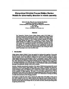
Figure 1 and Figure 2 plot the true density (red solid) and the 100 predictive densities (blue dot) given by the SUGS algorithm in case 1 for n = 500 and n = 5, 000, respectively. Clearly, the predictive densities are very close to the true density. Table 1 shows the average of 100 KLs of the proposed density estimates and the kernel density estimates relative to the 13
true density. The results in Table 1 suggest that the proposed density estimates are closer to the true density than the kernel density estimates. Table 1: Average of the Kullbuck-Leibler divergences in simulation 1. n = 500 n = 5000 SUGS
0.0125
0.0045
Kernel
0.0511
0.0112
Figures 3 and 4 plot the true density (red solid) and the 100 predictive densities (blue dot) given by the SUGS algorithm in case 2 for n = 500 and n = 5, 000, respectively. Again, the SUGS algorithm produces close predictive densities to the true density. Table 2 lists the average of KLs for the second case, with both SUGS and the typical kernel estimator working very well when the true model is a single normal. Table 2: Average of the Kullbuck-Leibler divergences in simulation 2. n = 500 n = 5000 SUGS
0.0026
0.0014
Kernel
0.0086
0.0013
Table 3 summarizes the estimated Bayes factors across the simulations. When data are generated from a mixture of normals in case 1, the Bayes factors provide decisive support in favor of the true model for both sample sizes as shown in Table 3. When data are generated from the null model as in simulation 2, the Bayes factors are in favor of the alternative only for 3/100 and 5/100 of the data sets. However, there is a tendency for the Bayes factor to be close to or equal to one under the null. This suggests that the Bayes factor is only consistent under the alternative, which is not surprising given the flexibility of the alternative model. Interestingly, the density estimates are still close to the true density even in the few cases in which the alternative is incorrectly favored. 14
Table 3: Performance of Bayes factor under null and alternative models. n case 1 case 2
BF < 1 BF = 1 1 < BF ≤ 100 BF > 100
500
0
0
0
100
5000
0
0
0
100
500
12
85
2
1
5000
2
93
1
4
The SUGS algorithm was very fast. In both case 1 and case 2, the analyses for all 100 simulated data sets were completed within 4 minutes for sample size 500 and in approximately 10 minutes for sample size 5,000. All programs were implemented in Matlab version 7.3 running on Dell desktop with Intel(R) Xeon (R) CPU and 3.00GB of RAM. 6.
Application
We applied the SUGS algorithm to three data examples. The first two are galaxy data and enzyme data, which have been studied thoroughly by many people in the literature and are available at www.stats.bris.ac.uk/∼peter/mixdata. The third is gestational age at delivery data from the Collaborative Perinatal Project (CPP), which was a very large epidemiologic study conducted in the 1960s and 70s. The CPP data and documentation are available at ftp://sph-ftp.jpsph.edu/cpp/ provided by John Hopkins University School of Public Health. Here we focus on 34,178 pregnancies that had their gestational ages at delivery (GADs) recorded in the the CPP data, which provide a large sample size example. The galaxy data are a commonly used example in assessing methods for Bayesian density estimation and clustering, e.g., Roeder (1990), Escobar and West (1995) and Richardson and Green (1997) among others. The data contain measured velocities of 82 galaxies from 6 well-separated conic sections of space. Using the default priors mentioned above, the SUGS algorithm gives three separated clusters, which agrees with the optimal partition obtained in Lau and Green (2007) based on the expected posterior loss function. Figure 5 shows the 15
predictive density under this partition. Taking b = 0.1 in SUGS results in a partition with 5 clusters and the corresponding predictive density is shown in Figure 6, which is similar to the results in Escobar and West (1995) and Richardson and Green (1997). The sensitivity to the prior for b is not surprising given the small sample size. The enzyme data record enzyme activities in blood for 245 individuals. One interest in analyzing this data set is the identification of subgroups of slow or fast metabolizers as a marker of genetic polymorphisms (Richardson and Green, 1997). Bechtel et al. (1993) concluded that the distribution is a mixture of two skewed distributions based on a maximum likelihood analysis. Richardson and Green (1997) analyzed the data using Bayesian normal mixtures with an unknown number of components. The application of the SUGS algorithm on the enzyme data gives a partition of 3 clusters. The predictive density shown in Figure 7 agrees closely with the findings in the above mentioned papers. Alternative prior specifications yield similar results. Table 4: The frequency of observations in categories of each covariate. value x1 (race) x2 (sex) x3 (smoke) x4 (age) 0
51.23%
49.72%
48.51%
7.72%
1
48.77%
50.28%
51.49%
92.28%
For the third example, we consider the GADs in weeks for 34,178 births in the CPP. We are interested in the relationship of GAD and the covariates race, sex, maternal smoking status during pregnancy, and maternal age. We use indicators X1 , X2 , X3 , and X4 to denote these four variables, with 1 indicating black, female, smoker, and maternal age less than 35, respectively, and with 0 indicating non-black, male, non-smoker, and maternal age no less than 35, respectively. Table 4 gives the observed frequencies for these covariates. The distribution of GAD is known to be non-normal and have heavy left tails by previous research, for example, Smith (2001) among others. In the following, we apply the proposed SUGS 16
algorithm on this data set. The left tail behavior of the distribution of GAD corresponding to premature deliveries is particularly of interest. Let zi = (1 xi1 xi2 xi3 xi4 )0 and yi denote the GAD for subject i. We consider the following model: yi ∼ N (z0i β i , τi−1 ),
(β i , τi )|P ∼ P,
P ∼ DP (αP0 )
P0 (β, τ ) = N (β; ξ, Ψτ −1 )Ga(τ ; a, b), where β i = (βi0 βi1 βi2 βi3 βi4 )0 denotes the random effects of intercept and covariates for subject i. To apply SUGS, we set ξ = 0, Ψ = n(zz0 )−1 , a = 1 and b = 1, where z = (z1 , · · · , zn )0 . In terms of computational speed, the analysis was completed within a few seconds for the Galaxy and enzyme data, while a single cycle of computation took approximately one minute for the CPP data. Figure 8 shows the estimated predictive densities and cumulative distribution functions of GAD for non-black babies and black babies controlling other covariates equal to zero. As seen in Figure 8, the predictive density of GAD for black babies is shifted left by around 1 week compared to the density of GAD for non-blacks. This result suggests that black babies are more likely to be born premature than non-black babies. Here, we only show the comparison of densities and CDFs of GAD for different race groups, and the corresponding densities and CDFs of GAD for different other covariate groups are very close (not shown). Note that SUGS will produce clusters of subjects having identical coefficients for the different predictors. Table 5 summarizes the results of the cluster-specific coefficients in the original data scale given by SUGS, including the posterior means and the corresponding 95% credible intervals. Table 5 also presents the sample mean of GAD and the number of subjects for each cluster in the last two rows. Clearly, the four clusters represent different groups of babies with the first cluster at the right tail of the distribution of GAD and the third and fourth clusters at the left tail. Cluster 2 is the dominant cluster containing about 17
Table 5: Cluster-specific coefficients obtained by SUGS.
β0 β1 β2 β3 β4 y¯j nj
cluster 1 cluster 2 cluster 3 cluster 4 48.26 (48.19, 48.32) 39.88 (39.88, 39.88) 31.40 (31.36, 31.44) 19.98 (16.19, 23.77) −0.01 (−0.02, 0.01) −0.70 (−0.70, −0.70) −1.62 (−1.63, −1.61) −3.28 (−4.43, −2.12) −0.11 (−0.12, −0.09) 0.12 (0.12, 0.12) 0.05 (0.04, 0.06) −0.56 (−1.48, 0.37) 0.03 (0.02, 0.05) 0.02 (0.01, 0.02) 0.04 (0.03, 0.048) 0.16 (−0.83, 1.14) 0.04 (−0.02, 0.10) 0.15 (0.15, 0.15) 1.06 (1.03, 1.096) 1.52 (−1.01, 4.04) 48.28 39.75 31.39 18.42 385 32024 1702 67
94% babies and the covariate effects are all significant in this cluster due to the extremely large sample size. Seen across the clusters, the effect of black race on GAD tends to increase in the clusters corresponding to lower GAD babies. This implies an interaction in which black race has a significant impact in shifting GAD slightly for full term deliveries, with a larger impact on timing of premature deliveries. 7.
Discussion
We have proposed a fast algorithm for posterior computation and model selection in Dirichlet process mixture models. The proposed SUGS approach is very fast and can be implemented easily in very large data sets when priors are chosen to be conjugate. In the simulations and real data examples we considered, we obtained promising results. Extensions to nonconjugate cases are conceptually straightforward. In such cases, instead of obtaining the exact marginal likelihoods conditional on the allocation to clusters, one can utilize an approximation. A promising strategy for many models would be to use a Laplace approximation. The performance of such an approach remains to be evaluated. Although our focus was on DPMs, the same type of approach can conceptually be applied in a much broader class of models, including species sampling models and general product partition models. 18
Acknowledgments This research was supported by the Intramural Research Program of the NIH, National Institute of Environmental Health Sciences. The authors would like to thank Richard Maclehose and Dave Kessler for their helpful comments. Appendix: Description of the predictive distribution Suppose that (y | x, β, τ ) ∼ N (x0 β, τ −1 ) with π(β, τ ) = Np (β; ξ, Ψτ −1 ) G(τ ; a, b) the prior. Then, the marginal likelihood of y given x follows the non-central t distribution: µ
Γ((ν + 1)/2) 1 1 + 2 (y − µy )2 f (y | x) = 1/2 (πν) Γ(ν/2)σ σ ν
¶−(ν+1)/2
= tν (y; µy , σ 2 ),
(15)
b = (Ψ−1 + xx0 )−1 , where ν = 2a is the degrees of freedom, Ψ b −1 ξ x0 ΨΨ µy = b 1 − x0 Ψx
µ
b −1 )ξ 1 2b + ξ 0 (Ψ−1 − Ψ−1 ΨΨ and σ = − µ2y , b 0 ν 1 − x Ψx 2
with µy the mean and σ 2 ν/(ν − 2) the variance for ν > 2. References Barry, D. and Hartigan, J.A. (1992), “Product Partition Models for Change Point Problems,” Annals of Statistics, 20, 260-279. Basu, S. and Chib, S. (2003), “Marginal likelihood and Bayes factors for Dirichlet process mixture models,” Journal of the American Statistical Association, 98, 224-235. Bechtel, Y.C., Bona¨ıti-Pelli´e, C., Poisson, N., Magnette, J. and Bechtel, P.R. (1993) “A Population and Family Study of N-acetyltransferase Using Caffeine Urinary Metabolites,” Clin. Pharm. Therp., 54, 134-141. Blackwell, D. and MacQueen, J. (1973), “Ferguson Distributions Via Polya Urn Schemes,” Annals of Statistics, 1, 353-355.
19
Blei, D.M. and Jordan, M.I. (2006), “Variational Inference for Dirichlet Process Mixtures,” Bayesian Analysis, 1, 121-144. Bowman, A.W. and Azzalini, A. (1997), “Applied Smoothing Techniques for Data Analysis,” Oxford Univeristy Press. Bush, C.A. and MacEachern, S.N. (1996), “A Semiparametric Bayesian Model for Randomized Block Designs,” Biometrika, 83, 175-185. Dahl, D.B. (2007), “Model Clustering in a Class of Product Partition Models,” Journal of Computational and Graphical Statistics, under revision. Dunson, D.B. (2007), “Empirical Bayes Density Regression,” Statistica Sinica, 17, 481-504. Escobar, M.D. (1994), “Estimating Normal Means with a Dirichlet Process Prior,” Journal of the American Statistical Association, 89, 268-277. Escobar, M.D. and West, M. (1995), “Bayesian Density Estimation and Inference Using Mixtures,” Journal of the American Statistical Association, 90, 577-588. Ferguson, T.S. (1973), “A Bayesian Analysis of Some Nonparametric Problems,” Annals of Statistics, 1, 209-230. Ferguson, T.S. (1974), “Prior Distributions on Spaces of Probability Measures,” Annals of Statistics, 2, 615-629. Geisser, S. (1980), “Discussion on Sampling and Bayes Inference in Scientific Modeling and Robustness (by G.E.P. Box),” Journal of the Royal Statistical Society A, 143, 416-417. Geisser, S. and Eddy, W. (1979), “A Predictive Approach to Model Selection ,” Journal of the American Statistical Association, 74, 153-160.
20
Gelfand, A.E. and Dey, D.K. (1994), “Bayesian Model Choice: Asymptotics and Exact Calculations,” with discussion, Journal of the Royal Statistical Society B, 56, 501-514. Holmes, C.C, Denison, D.G.T, Ray, S. and Mallick, B.K. (2005), “Bayesian Prediction via Partitioning,” Journal of Computational and Graphical Statistics, 14, 811-830. Ishwaran, H. and James, L.F. (2001), “Gibbs Sampling Methods for Stick-breaking Priors,” Journal of the American Statistical Association, 101, 179-194. Ishwaran, H. and James, L.F. (2003) “Generalized Weighted Chinese Restaurant Processes for Species Sampling Mixture Models,” Statistica Sinica, 13, 1211-1235. Ishwaran, H. and Takahara, G. (2002), “Independent and Identically Distributed Monte Carlo Algorithms for Semiparametric Linear Mixed Models. Journal of the American Statistical Association 97, 1154-1166. Jain, S. and Neal, R.M. (2004) “A Split-merge Markov Chain Monte Carlo Procedure for the Dirichlet Process Mixture Model, ” Journal of Computational and Graphical Statistics, 13, 158-182. Kurihara, K., Welling, M. and Vlassis, N. (2006), “Accelerated Variational Dirichlet Mixture Models”, Advances in Neural Information Processing Systems 19 (NIPS 2006). Kurihara, K., Welling, M. and Teh, Y.W. (2007), “Collapsed variational Dirichlet process mixture models”, Twentieth International Joint Conference on Artificial Intelligence (IJCAI07). Lau, J.W. and Green, P.J. (2007), “Bayesian model based clustering procedures,” To appear in Journal of Computational and Graphical Statistics Lo, A.Y. (1984), “On a Class of Bayesian Nonparametric Estimates: I, Density Estimates,” Annals of Statistics, 12, 351-357. 21
Lo, A.Y., Brunner, L.J. and Chan, A.T. (1996), “Weighted Chinese Restaurant Processses and Bayesian Mixture Models,” Research Report 1, Hong Kong University of Science and Technology. MacEachern, S.N. (1994), “Estimating Normal Means with a Conjugate Style Dirichlet Process Prior,” Communications in Statistics: Simulation and Computation, 23, 727741. MacEachern, S.N., Clyde, M. and Liu, J.S. (1999), “Sequential Importance Sampling for Nonparametric Bayes Models: The Next Generation,” Canadian Journal of Statistics, 27, 251-267. Mukhopadhyay, N., Ghosh, J.K. and Berger, J.O. (2005), “ Some Bayesian Predictive Approaches to Model Selection,” Statistics & Probability Letters, 73, 369-379. Newton, M.A. and Zhang, Y. (1999), “A Recursive Algorithm for Nonparametric Analysis with Missing Data,” Biometrika, 86, 15-26. Pettit, L.I. (1990), “The Conditional Predictive Ordinate for the Normal Distribution,” Journal of the Royal Statistical Society B, 52, 175-184. Quintana, F.A. and Iglesias, P.L. (2003), “Bayesian Clustering and Product Partition Models,” Journal of the Royal Statistical Society B, 65, 557-574. Quintana, F.A. and Newton, M.A. (2000), “Computational Aspects of Nonparametric Bayesian Analysis with Applications to the Modeling of Multiple Binary Sequences,” Journal of Computational and Graphical Statistics, 9, 711-737. Richardson, S. and Green, P.J. (1997), “On Bayesian Analysis of Mixtures with an Unknown Number of Components,” Journal of Royal Statistical Society B , 59, 731-792.
22
Roeder, K (1990), “Density Estimation With Confidence Sets Exemplified by Superclusters and Voids in the Galaxies,” Journal of the American Statistical Association, 85, 617624. Sinha, D., Chen, M.H. and Ghosh, S.K. (1999), “Bayesian Analysis and Model Selection for Interval-censored Survival Data,” Biometrics, 55, 585-590. Smith, G.C.S. (2001), “Use of Time to Event Analysis to Estimate the Normal Duration of Human Pregnancy”, HUMAN REPRODUCTION 16, 1497-1500. Stephens, M. (2000), “Dealing with Label Switching in Mixture Models,” Journal of the Royal Statistical Society B, 62, 795-809. Tao, H., Palta, M., Yandell, B.S. and Newton, M.A. (1999), “An Estimation Method for the Semiparametric Mixed Effects Model,” Biometrics, 55, 102-110. Wang, B. and Titterington, M. (2005), “Inadequacy of Interval Estimates Corresponding to Variational Bayesian Approximations,” In AISTATS05 (eds R.G. Cowell and Z. Ghahramani), Society for Artificial Intelligence and Statistics. West, M., Miller, P. and Escobar, M.D. (1994) “Hierarchical priors and mixture models, with application in regression and density estimation,” Aspects of Uncertainty: A Tribute to D.V. Lindley 363-386. Zhang, J., Ghahramani, Z. and Yang, Y. (2005), “A Probabilistic Model for Online Document Clustering with Application to Novelty Detection”, In Advances in Neural Information Processing Systems 17. (NIPS-2004).
23
0.5 0.45 0.4
Density g(y)
0.35 0.3 0.25 0.2 0.15 0.1 0.05 0
−4
−2
0
2
4
6
y
Figure 1: Density estimation in simulation 1. The estimated densities (green dotted) from 100 data sets and the true density (red solid) when sample size is 500.
0.45 0.4 0.35
Density g(y)
0.3 0.25 0.2 0.15 0.1 0.05 0
−4
−2
0
2
4
6
y
Figure 2: Density estimation in simulation 1. The estimated densities (green dotted) from 100 data sets and the true density (red solid) when sample size is 5000.
24
0.7
0.6
Density g(y)
0.5
0.4
0.3
0.2
0.1
0 −3
−2
−1
0 y
1
2
3
Figure 3: Density estimation in simulation 2. The estimated densities (green dotted) from 100 data sets and the true density (red solid) when sample size is 500.
0.7
0.6
Density g(y)
0.5
0.4
0.3
0.2
0.1
0 −3
−2
−1
0 y
1
2
3
Figure 4: Density estimation in simulation 2. The estimated densities (green dotted) from 100 data sets and the true density (red solid) when sample size is 5000.
25
0.25
0.2
0.15
0.1
0.05
0
5
10
15
20
25
30
35
40
Figure 5: Predictive density estimation, histogram, and plots of galaxy data, b = 1.
0.25
0.2
0.15
0.1
0.05
0
5
10
15
20
25
30
35
40
Figure 6: Predictive density estimation, histogram, and plots of galaxy data, b = 0.1.
26
3.5
3
2.5
2
1.5
1
0.5
0 −0.5
0
0.5
1
1.5
2
2.5
3
3.5
Figure 7: Predictive density estimation, histogram, and plots of enzyme data, b = 0.1.
27
0.2 0.15
non−black black
0.1 0.05 0 20
25
30
35
40
45
50
30
35
40
45
50
1 0.8
non−black black
0.6 0.4 0.2 0 20
25
Figure 8: Top: Densities of GAD for black race (blue dashed) and other race (red solid). Bottom: Cumulative distribution functions of GAD for black race (blue dashed) and other race (red solid). 28