Stability and Convergence of an Effective Finite Element Method for

Hindawi Publishing Corporation Abstract and Applied Analysis Volume 2013, Article ID 857205, 10 pages http://dx.doi.org/10.1155/2013/857205

Research Article Stability and Convergence of an Effective Finite Element Method for Multiterm Fractional Partial Differential Equations Jingjun Zhao, Jingyu Xiao, and Yang Xu Department of Mathematics, Harbin Institute of Technology, Harbin 150001, China Correspondence should be addressed to Yang Xu; [email protected] Received 11 December 2012; Revised 3 February 2013; Accepted 6 February 2013 Academic Editor: Dragos¸-P˘atru Covei Copyright © 2013 Jingjun Zhao et al. This is an open access article distributed under the Creative Commons Attribution License, which permits unrestricted use, distribution, and reproduction in any medium, provided the original work is properly cited. A finite element method (FEM) for multiterm fractional partial differential equations (MT-FPDEs) is studied for obtaining a numerical solution effectively. The weak formulation for MT-FPDEs and the existence and uniqueness of the weak solutions are obtained by the well-known Lax-Milgram theorem. The Diethelm fractional backward difference method (DFBDM), based on quadrature for the time discretization, and FEM for the spatial discretization have been applied to MT-FPDEs. The stability and convergence for numerical methods are discussed. The numerical examples are given to match well with the main conclusions.

where the operator 𝑃(𝐶𝐷𝑡 )𝑢(𝑡, 𝑥) is defined as

1. Introduction In recent years, the numerical treatment and supporting analysis of fractional order differential equations has become an important research topic that offers great potential. The FEMs for fractional partial differential equations have been studied by many authors (see [1–3]). All of these papers only considered single-term fractional equations, where they only had one fractional differential operator. In this paper, we consider the MT-FPDEs, which include more than one fractional derivative. Some authors also considered solving linear problems with multiterm fractional derivatives (see [4, 5]). This motivates us to consider their effective numerical solutions for such MT-FPDEs, which have been proposed in [6, 7]. Let Ω = (0, 𝑋)𝑑 , where 𝑑 ≥ 1 is the space dimension. We consider the MT-FPDEs with the Caputo time fractional derivatives as follows: 𝑃 (𝐶𝐷𝑡 ) 𝑢 (𝑡, 𝑥) − Δ 𝑥 𝑢 (𝑡, 𝑥) = 𝑓 (𝑡, 𝑥) , 𝑢 (0, 𝑥) = 𝑢0 (𝑥) , 𝑢 (𝑡, 𝑥) = 0,

𝑡 ∈ [0, 𝑇] , 𝑥 ∈ Ω, (1)

𝑥 ∈ Ω,

𝑡 ∈ [0, 𝑇] , 𝑥 ∈ 𝜕Ω,

(2) (3)

𝛼

𝑠

𝛼

𝑃 (𝐶𝐷𝑡 ) 𝑢 (𝑡, 𝑥) = ( 𝐶0𝐷𝑡 + ∑𝑎𝑖 𝐶0𝐷𝑡 𝑖 ) 𝑢 (𝑡, 𝑥) ,

(4)

𝑖=1

with 0 < 𝛼𝑠 < 𝛼𝑠−1 < ⋅ ⋅ ⋅ < 𝛼1 < 𝛼 < 1 and {𝑎𝑖 > 0}𝑠𝑖=1 . Here 𝐶0𝐷𝑡𝛼 𝑢(𝑡, 𝑥) denotes the left Caputo fractional derivative with respect to the time variable 𝑡 and Δ 𝑥 denotes the Laplace operator with respect to the space variable 𝑥. Some numerical methods have been considered for solving the multiterm fractional differential equations. In [8], Liu et al. investigate some effective numerical methods for time fractional wave-diffusion and diffusion equations: 𝐶 𝛼 0 𝐷𝑡 𝑢 (𝑡, 𝑥)

− 𝑘Δ 𝑥 𝑢 (𝑡, 𝑥) = 𝑓 (𝑡, 𝑥) ,

0 < 𝑥 < 𝐿, 𝑡 > 0, (5)

where 𝑘 and 𝐿 are arbitrary positive constants and 𝑓(𝑡, 𝑥) is a sufficiently smooth function. The authors consider the implicit finite difference methods (FDMs) and prove that it is unconditionally stable. The error estimate of the FDM is 𝑂(Δ𝑡 + Δ𝑡2−𝛼 + Δ𝑥), where Δ𝑡 and Δ𝑥 are the time and space step size, respectively. They also investigate the fractional predictor-corrector methods (FPCMs) of the AdamsMoulton methods for multiterm time fractional differential equations (1) with order {𝛼𝑖 }𝑖=1,...,𝑠 by solving the equivalent

2

Abstract and Applied Analysis

Volterra integral equations. The error estimate of the FPCM is 𝑂(Δ𝑡 + Δ𝑡1+min{𝛼𝑙 } + Δ𝑥2 ). In recent years, there are some articles for the predictor-correction method for initial-value problems (see [9–14]). For the application of the FDMs, there have been many research articles as follows. In [15–20], Simos et al. investigate the numerical methods for solving the Schr¨odinger equation. In [21–24], the Runge-Kutta methods are considered and applied to get the numerical solution of orbital problems. For long-time integration, the NewtonCotes formulae are considered in [25–27]. In [28], Badr investigate the FEM for linear multiterm fractional differential equations with one variable as follows: 𝐶 1+𝛼 0 𝐷𝑡 𝑢 (𝑡)

Let 𝐶∞ (0, 𝑇) denote the space of infinitely differentiable functions on (0, 𝑇) and 𝐶0∞ (0, 𝑇) denote the space of infinitely differentiable functions with compact support in (0, 𝑇). We use the expression 𝐴 ≲ 𝐵 to mean that 𝐴 ≤ 𝑐𝐵 when 𝑐 is a positive real number and use the expression 𝐴 ≅ 𝐵 to mean that 𝐴 ≲ 𝐵 ≲ 𝐴. Let 𝐿 2 (Q) be the space of measurable functions whose square is the Lebesgue integrable in Q which may denote a domain Q = 𝐼 × Ω, 𝐼 or Ω. Here time domain 𝐼 := (0, 𝑇) and space domain Ω := (0, 𝑋). The inner product and norm of 𝐿 2 (Q) are defined by (𝑢, V)𝐿 2 (Q) := ∫ 𝑢V𝑑Q, Q

𝑠

+ ∑𝐴 𝑖 (𝑥) 𝐷𝛼𝑖 𝑢 (𝑥) = 𝑓 (𝑡) ,

𝛼 ≤ 𝑛,

𝑖=1

where 𝐴 𝑖 (𝑥) are known functions. The author gives the details of the modified Galerkin method for the above equations and makes the numerical example for checking the numerical method. In [29], Ford et al. consider the FEM for (5) with singular fractional order and obtain the error estimate 𝑂(Δ𝑡2−𝛼 + Δ𝑥2 ). In this paper, we follow the work in [29] and consider the FEM for solving MT-FPDEs (1)–(3). Then, we prove the stability and convergence of the FEM for MTFPDEs and make the error estimate. The paper is organized as follows. In Section 2, the weak formulation of the MT-FPDEs is given and the existence and uniqueness results for such problems are proved. In Section 3, we consider the convergence rate of time discretization of MT-FPDEs, based on the Diethelm fractional backward difference method (DFBDM). In Section 4, we propose an FEM based on the weak formulation and carry out the error analysis. In Section 5, the stability of this method is proven. Finally, the numerical examples are considered for matching well with the main conclusions.

For any real 𝜎 > 0, we define the spaces 𝑙 𝐻0𝜎 (Q) and 𝐻0𝜎 (Q) to be the closure of 𝐶0∞ (Q) with respect to the norms ‖V‖ 𝑙 𝐻0𝜎 (Q) , and ‖V‖ 𝑟 𝐻0𝜎 (Q) respectively, where 𝑟

‖V‖ 𝑙 𝐻0𝜎 (Q) := (‖V‖2𝐿 2 (Q) + |V|2𝑙 𝐻𝜎 (Q) )

(i) The left Caputo derivatives: :=

𝑡 1 1 𝑑𝑛 ( V (𝜏)) 𝑑𝜏. (7) ∫ Γ (𝑛 − 𝛼) 0 (𝑡 − 𝜏)𝛼−𝑛+1 𝑑𝜏𝑛

1/2

0

,

󵄩 𝜎 󵄩2 |V|2𝑙 𝐻𝜎 (Q) := 󵄩󵄩󵄩󵄩 𝑅0 𝐷𝑡 V󵄩󵄩󵄩󵄩𝐿 (Q) , 0 2 1/2

‖V‖ 𝑟 𝐻0𝜎 (Q) := (‖V‖2𝐿 2 (Q) + |V|2𝑟 𝐻0𝜎 (Q) )

(11) ,

󵄩 𝜎 󵄩2 |V|2𝑟 𝐻0𝜎 (Q) := 󵄩󵄩󵄩󵄩 𝑅𝑡 𝐷𝑇 V󵄩󵄩󵄩󵄩𝐿 (Q) . 2 In the usual Sobolev space 𝐻0𝜎 (Q), we also have the definition 1/2

‖V‖𝐻0𝜎 (Q) := (‖V‖2𝐿 2 (Q) + |V|2𝐻0𝜎 (Q) )

,

𝜎

|V|2𝐻0𝜎 (Q)

:=

2. Existence and Uniqueness Let Γ(⋅) denote the gamma function. For any positive integer 𝑛 and 𝑛 − 1 < 𝛼 < 𝑛, the Caputo derivative are the RiemannLiouville derivative are, respectively, defined as follows [30].

(10)

∀𝑢, V ∈ 𝐿 2 (Q) .

(6)

𝛼𝑖 < 𝑛 − 1, 0 < 𝑡 < 1,

𝐶 𝛼 0 𝐷𝑡 V (𝑡)

‖𝑢‖𝐿 2 (Q) := (𝑢, 𝑢)1/2 𝐿 2 (Q) ,

( 𝑅0 𝐷𝑡 V, 𝑅𝑡 𝐷𝑇𝜎 V)𝐿

(12) 2 (Q)

cos (𝜋𝜎)

.

From [3], for 𝜎 > 0, 𝜎 ≠ 𝑛 − 1/2, the spaces 𝑙 𝐻0𝜎 (Q), 𝐻0𝜎 (Q), and 𝐻0𝜎 (Q) are equal, and their seminorms are all equivalent to | ⋅ |𝐻0𝜎 (Q) . We first recall the following results. 𝑟

Lemma 1 (see [3]). Let 0 < 𝜃 < 2, 𝜃 ≠ 1. Then for any 𝑤, V ∈ 𝐻0𝜃/2 (0, 𝑇), then 𝜃

( 𝑅0 𝐷𝑡 𝑤, V)

𝜃/2

𝐿 2 (0,𝑇)

= ( 𝑅0 𝐷𝑡 𝑤, 𝑅𝑡 𝐷𝑇𝜃/2 V)

𝐿 2 (0,𝑇)

.

(13)

(ii) The left Riemann-Liouville derivatives: 𝑅 𝛼 0 𝐷𝑡 V (𝑡)

𝑑𝑛 𝑡 V (𝜏) 1 := 𝑑𝜏. ∫ 𝑛 Γ (𝑛 − 𝛼) 𝑑𝑡 0 (𝑡 − 𝜏)𝛼−𝑛+1

From [3], we define the following space: (8)

∩ 𝐻𝛼𝑠 /2 (𝐼, 𝐿 2 (Ω)) ∩ 𝐿 2 (𝐼, 𝐻01 (Ω))

(iii) The right Riemann-Liouville derivatives: 𝑅 𝛼 𝑡 𝐷𝑇 V (𝑡)

:=

V (𝜏) (−1)𝑛 𝑑𝑛 𝑇 𝑑𝜏. ∫ Γ (𝑛 − 𝛼) 𝑑𝑡𝑛 𝑡 (𝜏 − 𝑡)𝛼−𝑛+1

𝐵𝛼/2 (𝐼 × Ω) = 𝐻𝛼/2 (𝐼, 𝐿 2 (Ω)) ∩ 𝐻𝛼1 /2 (𝐼, 𝐿 2 (Ω)) ∩ ⋅ ⋅ ⋅

(9)

= 𝐻𝛼/2 (𝐼, 𝐿 2 (Ω)) ∩ 𝐿 2 (𝐼, 𝐻01 (Ω)) . (14)

Abstract and Applied Analysis

3

Here 𝐵𝛼/2 (𝐼 × Ω) is a Banach space with respect to the following norm: ‖V‖𝐵𝛼/2 (𝐼×Ω) =

(‖V‖2𝐻𝛼/2 (𝐼,𝐿 (Ω)) 2

+

‖V‖2𝐿 2 (𝐼,𝐻1 (Ω)) ) 0

1/2

,

(15)

where 𝐻𝛼/2 (𝐼, 𝐿 2 (Ω)) := {V; ‖V(𝑡, ⋅)‖𝐿 2 (Ω) ∈ 𝐻𝛼/2 (𝐼)}, endowed with the norm 󵄩 󵄩 ‖V‖𝐻𝛼/2 (𝐼,𝐿 2 (Ω)) := 󵄩󵄩󵄩󵄩‖V (𝑡, ⋅)‖𝐿 2 (Ω) 󵄩󵄩󵄩󵄩𝐻𝛼/2 (𝐼) . (16) Based on the relation equation between the left Caputo and the Riemann-Liouville derivative in [31], we can translate the Caputo problem to the Riemann-Liouville problem. Then, we consider the weak formulation of (1) as follows. For 𝑓 ∈ 𝐵𝛼/2 (𝐼 × Ω)󸀠 , find 𝑢(𝑡, 𝑥) ∈ 𝐵𝛼/2 (𝐼 × Ω) such that V ∈ 𝐵𝛼/2 (𝐼 × Ω) ,

A (𝑢, V) = F (V) ,

(17)

where the bilinear form is, by Lemma 1, 𝛼/2

A (𝑢, V) := ( 𝑅0 𝐷𝑡 𝑢, 𝑅𝑡 𝐷𝑇𝛼/2 V) 𝑠

𝛼𝑖 /2

+ ∑𝑎𝑖 ( 𝑅0 𝐷𝑡 𝑖=1

𝛼 /2

𝐿 2 (𝐼×Ω)

(18)

+ (∇𝑥 𝑢, ∇𝑥 V)𝐿 2 (𝐼×Ω) , and the functional is F(V) := (𝑓, V)𝐿 2 (𝐼×Ω) , 𝑓(𝑡, 𝑥) := 𝑓(𝑡, 𝑥)+ (𝑢0 (𝑥)𝑡−𝛼 /Γ(1 − 𝛼)) + ∑𝑠𝑖=1 𝑎𝑖 (𝑢0 (𝑥)𝑡−𝛼𝑖 /Γ(1 − 𝛼𝑖 )). Based on the main results in Subsection 3.2 in [32], we can prove the following existence and uniqueness theorem. Theorem 2. Assume that 0 < 𝛼 < 1 and 𝑓 ∈ 𝐵𝛼/2 (𝐼 × Ω)󸀠 . Then the system (17) has a unique solution in 𝐵𝛼/2 (𝐼 × Ω). Furthermore, 󵄩 󵄩 ‖𝑢‖𝐵𝛼/2 (𝐼×Ω) ≲ 󵄩󵄩󵄩󵄩𝑓󵄩󵄩󵄩󵄩𝐵𝛼/2 (𝐼×Ω)󸀠 .

(19)

Proof. The existence and uniqueness of the solution of (17) is guaranteed by the well-known Lax-Milgram theorem. The continuity of the bilinear form A and the functional F is obvious. Now we need to prove the coercivity of A in the space 𝐵𝛼/2 (𝐼 × Ω). From the equivalence of 𝑙 𝐻0𝛼 (𝐼 × Ω), 𝑟 𝛼 𝐻0 (𝐼 × Ω) and 𝐻0𝛼 (𝐼 × Ω), for all 𝑢, V ∈ 𝐵𝛼/2 (𝐼 × Ω), using the similar proof process in [32], we obtain 𝛼/2

A (V, V) ≳ ( 𝑅0 𝐷𝑡 V, 𝑅0 𝐷𝑡𝛼/2 V) 𝑠

𝛼𝑖 /2

+ ∑𝑎𝑖 ( 𝑅0 𝐷𝑡 𝑖=1

𝐿 2 (𝐼×Ω) 𝛼 /2

V, 𝑅0 𝐷𝑡 𝑖 V)

In this section, we consider DFBDM for the time discretization of (1)–(3), which is introduced in [33] for fractional ordinary differential equations. We can obtain the convergence order for the time discretization for the MT-FPDEs. Let 𝐴 = −Δ 𝑥 , 𝐷(𝐴) = 𝐻01 (Ω) ∩ 𝐻2 (Ω). Let 𝑢(𝑡), 𝑓(𝑡), and 𝑢(0) denote the one-variable functions as 𝑢(𝑡, ⋅), 𝑓(𝑡, ⋅), and 𝑢(0, ⋅), respectively. Then (1) can be written in the abstract form, for 0 < 𝑡 < 𝑇, 0 < 𝛼𝑠 < ⋅ ⋅ ⋅ < 𝛼1 < 𝛼 < 1, with initial value 𝑢(0) = 𝑢0 . Now we have 𝑅 𝛼 0 𝐷𝑡

𝑠

𝐿 2 (𝐼×Ω)

(20)

𝛼

[𝑢 − 𝑢0 ] (𝑡) + ∑𝑎𝑖 𝑅0 𝐷𝑡 𝑖 [𝑢 − 𝑢0 ] (𝑡) + 𝐴𝑢 (𝑡) = 𝑓 (𝑡) . 𝑖=1

(21) Let 0 = 𝑡0 < 𝑡1 < ⋅ ⋅ ⋅ < 𝑡𝑁 = 𝑇 be a partition of [0, 𝑇]. Then, for fixed 𝑡𝑗 , 𝑗 = 1, 2, . . . , 𝑁, we have 𝑅 𝛼 0 𝐷𝑡

𝐿 2 (𝐼×Ω)

𝑢, 𝑅𝑡 𝐷𝑇𝑖 V)

3. Time Discretization and Convergence

[𝑢 − 𝑢0 ] (𝑡𝑗 ) =

1

Γ (−𝛼)

∫ 𝑔 (𝜏) 𝜏−1−𝛼 𝑑𝜏,

(22)

0

where 𝑔(𝜏) = 𝑢(𝑡𝑗 −𝑡𝑗 𝜏)−𝑢0 . Here, the integral is a Hadamard finite-part integral in [33] and [34]. Now, for every 𝑗, we replace the integral by a firstdegree compound quadrature formula with equispaced nodes 0, (1/𝑗), (2/𝑗), . . . , 1 and obtain 𝑗

1 𝑘 (𝛼) 𝑔 ( ) + 𝑅𝑗(𝛼) (𝑔) , ∫ 𝑔 (𝜏) 𝜏−1−𝛼 𝑑𝜏 = ∑ 𝛼𝑘𝑗 𝑗 0 𝑘=0

(23)

(𝛼) are where the weights 𝛼𝑘𝑗 (𝛼) 𝛼 (1 − 𝛼) 𝑗−𝛼 𝛼𝑘𝑗

−1, for 𝑘 = 0, { { = {2𝑘1−𝛼 −(𝑘−1)1−𝛼 −(𝑘+1)1−𝛼 , for 𝑘 = 1, 2, . . . , 𝑗−1, { 1−𝛼 −𝛼 1−𝛼 {(𝛼−1) 𝑘 −(𝑘−1) +𝑘 , for 𝑘 = 𝑗, (24) and the remainder term 𝑅𝑗(𝛼) (𝑔) satisfies ‖𝑅𝑗(𝛼) (𝑔)‖ 𝛾𝛼 𝑗𝛼−2 sup0≤𝑡≤𝑇 ‖𝑔󸀠󸀠 (𝑡)‖, where 𝛾𝛼 > 0 is a constant. (𝛼) (𝛼) Thus, for 𝜔𝑘𝑗 = 𝑗−𝛼 𝛼𝑘𝑗 /Γ(−𝛼), we have 𝑅 𝛼 0 𝐷𝑡

≤

𝑗

(𝛼) [𝑢 − 𝑢0 ] (𝑡𝑗 ) = Δ𝑡−𝛼 ∑ 𝜔𝑘𝑗 (𝑢 (𝑡𝑗 − 𝑡𝑘 ) − 𝑢 (0)) 𝑘=0

+ (∇𝑥 𝑢, ∇𝑥 V)𝐿 2 (𝐼×Ω) ≳ ‖V‖2𝐵𝛼/2 (𝐼×Ω) . Then we take V = 𝑢 in (17) to get ‖𝑢‖2𝐵𝛼/2 (𝐼×Ω) ≲ (𝑓, 𝑢)𝐿 2 (𝐼×Ω) by the Schwarz inequality and the Poincar´e inequality.

𝑡𝑗−𝛼

+

𝑡𝑗−𝛼 Γ (−𝛼)

𝑅𝑗(𝛼) (𝑔) . (25)

4

Abstract and Applied Analysis Let 𝑡 = 𝑡𝑗 , we can write (21) as

Let ‖ ⋅ ‖ denote the 𝐿 2 -norm, then we have

𝑗

(𝛼) Δ𝑡−𝛼 ∑ 𝜔𝑘𝑗 (𝑢 (𝑡𝑗 − 𝑡𝑘 ) − 𝑢 (0))

󵄩󵄩 𝑗 󵄩󵄩 󵄩󵄩𝑒 󵄩󵄩 ≤ 󵄩 󵄩

𝑘=0

𝑗

𝑠

(𝛼 )

+ ∑𝑎𝑖 Δ𝑡−𝛼𝑖 ∑ 𝜔𝑘𝑗 𝑖 (𝑢 (𝑡𝑗 − 𝑡𝑘 ) − 𝑢 (0)) + 𝐴𝑢 (𝑡𝑗 ) 𝑖=1

𝑗

= 𝑓 (𝑡𝑗 ) −

Γ (−𝛼)

𝑅𝑗(𝛼)

−𝛼𝑖

𝑡𝑗

𝑠

(𝑔) − ∑𝑎𝑖 𝑖=1

Γ (−𝛼𝑖 )

(𝛼𝑖 )

𝑅𝑗

(𝑔) ,

󵄩 󵄩 𝑠 Γ (−𝛼) 𝛼−𝛼𝑖 󵄩󵄩 (𝛼𝑖 ) 󵄩 + 󵄩󵄩󵄩󵄩𝑅𝑗(𝛼) (𝑔)󵄩󵄩󵄩󵄩 + ∑𝑎𝑖 𝑡𝑗 󵄩󵄩󵄩𝑅𝑗 (𝑔)󵄩󵄩󵄩󵄩 ) . Γ (−𝛼 ) 𝑖 𝑖=1 (30)

𝑗 = 1, 2, 3, . . . . (26) Denote 𝑈𝑗 as the approximation of 𝑢(𝑡𝑗 ) and 𝑓𝑗 = 𝑓(𝑡𝑗 ). We obtain the following equation: 𝑗

(𝛼) Δ𝑡−𝛼 ∑ 𝜔𝑘𝑗 (𝑈𝑗−𝑘 − 𝑈0 ) 𝑘=0

(27)

𝑠

𝑗

𝑖=1

𝑘=0

𝑗

𝑠 (𝛼) 󵄩 󵄩󵄩𝑒𝑗−𝑘 󵄩󵄩󵄩 + ∑𝑎 Δ𝑡𝛼−𝛼𝑖 Γ (−𝛼) ∑ 𝛼(𝛼𝑖 ) 󵄩󵄩󵄩𝑒𝑗−𝑘 󵄩󵄩󵄩 × ( ∑ 𝛼𝑘𝑗 󵄩󵄩 󵄩󵄩 󵄩 󵄩󵄩 𝑖 Γ (−𝛼𝑖 ) 𝑘=1 𝑘𝑗 󵄩 𝑖=1 𝑘=1

𝑘=0

𝑡𝑗−𝛼

󵄩󵄩 −1 󵄩 󵄩󵄩 󵄩󵄩 (𝛼) 𝑠 󵄩󵄩(𝛼 + ∑𝑎 Δ𝑡𝛼−𝛼𝑖 Γ (−𝛼) 𝛼(𝛼𝑖 ) + 𝐴𝑡𝛼 Γ (−𝛼)) 󵄩󵄩󵄩 󵄩󵄩 0𝑗 󵄩󵄩 𝑖 0𝑗 Γ (−𝛼𝑖 ) 󵄩󵄩 󵄩󵄩 𝑖=1 󵄩 󵄩

(𝛼 )

+ ∑𝑎𝑖 Δ𝑡−𝛼𝑖 ∑ 𝜔𝑘𝑗 𝑖 (𝑈𝑗−𝑘 − 𝑈0 ) + 𝐴𝑈𝑗 = 𝑓𝑗 . Lemma 3 (see [34]). For 0 < 𝛼 < 1, let the sequence {𝑑𝑗 }𝑗=1,2,... 𝑗−1

(𝛼) be given by 𝑑1 = 1 and 𝑑𝑗 = 1+𝛼(1−𝛼)𝑗−𝛼 ∑𝑘=1 𝛼𝑘𝑗 𝑑𝑗−𝑘 . Then, 𝛼 1 ≤ 𝑑𝑗 ≤ (sin(𝜋𝛼)/𝜋𝛼(1 − 𝛼))𝑗 , for 𝑗 = 1, 2, 3, . . . .

Note that 𝐴 is a positive definite elliptic operator with all (𝛼) of eigenvalues 𝜆 > 0. Since 𝛼0𝑗 < 0 and Γ(−𝛼) < 0, we have 󵄩󵄩 −1 󵄩 󵄩󵄩 󵄩󵄩 (𝛼) 𝑠 󵄩󵄩(𝛼 + ∑𝑎 Δ𝑡𝛼−𝛼𝑖 Γ (−𝛼) 𝛼(𝛼𝑖 ) + 𝐴𝑡𝛼 Γ (−𝛼)) 󵄩󵄩󵄩 󵄩󵄩 𝑖 󵄩󵄩󵄩 0𝑗 Γ (−𝛼𝑖 ) 0𝑗 󵄩󵄩 󵄩󵄩 𝑖=1 󵄩 −1 󵄩 󵄩󵄩󵄩 󵄩󵄩 Γ (−𝛼) (𝛼𝑖 ) 󵄩 (𝛼) 𝑠 󵄩 = sup 󵄩󵄩󵄩󵄩(𝛼0𝑗 + ∑𝑎𝑖 Δ𝑡𝛼−𝛼𝑖 𝛼0𝑗 + 𝜆𝑡𝛼 Γ (−𝛼)) 󵄩󵄩󵄩󵄩 Γ (−𝛼 ) 󵄩 󵄩󵄩 𝜆>0 󵄩 𝑖 𝑖=1 󵄩 󵄩 −1

𝑠

(𝛼) ≲ (− 𝛼0𝑗 − ∑𝑎𝑖 Δ𝑡𝛼−𝛼𝑖 𝑖=1

Γ (−𝛼) (𝛼𝑖 ) 𝛼 ) . Γ (−𝛼𝑖 ) 0𝑗 (31)

Let 𝑒𝑗 = 𝑢(𝑡𝑗 ) − 𝑈𝑗 denote the error in 𝑡𝑗 . Then we have the following error estimate. Theorem 4. Let 𝑈𝑗 and 𝑢(𝑡𝑗 ) be the solutions of (27) and (21), respectively. Then one has ‖𝑈𝑗 − 𝑢(𝑡𝑗 )‖ ≲ Δ𝑡2−𝛼 . Proof. Subtracting (27) from (26), we obtain the error equation −𝛼

Δ𝑡

𝑗

(𝛼) ∑ 𝜔𝑘𝑗 𝑘=0

=−

𝑗−𝑘

(𝑒

𝑠

0

−𝛼𝑖

− 𝑒 ) + ∑𝑎𝑖 Δ𝑡 𝑖=1

𝑡𝑗−𝛼

𝑠

Γ (−𝛼)

𝑅𝑗(𝛼) (𝑔) − ∑𝑎𝑖 𝑖=1

(𝛼 ) ∑ 𝜔𝑘𝑗 𝑖 𝑘=0

−𝛼𝑖

Γ (−𝛼𝑖 )

(𝑒

(𝛼𝑖 )

𝑅𝑗

𝑗−𝑘

0

𝑗

− 𝑒 ) + 𝐴𝑒

𝑘=1

𝑠 󵄩 (𝛼 ) 󵄩 + ∑𝛼𝑖 (1 − 𝛼𝑖 ) 𝑗−𝛼𝑖 ∑ 𝛼𝑘𝑗 𝑖 󵄩󵄩󵄩󵄩𝑒𝑗−𝑘 󵄩󵄩󵄩󵄩 𝑖=1

𝑘=1

󵄩 󵄩 + 𝛼 (1 − 𝛼) 𝛾𝛼 𝑛 sup 󵄩󵄩󵄩󵄩𝑢󸀠󸀠 󵄩󵄩󵄩󵄩 0≤𝑡≤𝑇

(32)

−2

(𝑔) . (28)

0

𝑗

󵄩󵄩 𝑗 󵄩󵄩 (𝛼) 󵄩 󵄩󵄩𝑒𝑗−𝑘 󵄩󵄩󵄩 󵄩󵄩𝑒 󵄩󵄩 ≤ 𝛼 (1 − 𝛼) 𝑗−𝛼 ∑ 𝛼𝑘𝑗 󵄩󵄩 󵄩󵄩 󵄩 󵄩 𝑗

𝑗

𝑡𝑗

Hence,

𝑠 󵄩 󵄩 + ∑𝛼𝑖 (1 − 𝛼𝑖 ) 𝛾𝛼𝑖 𝑛−2 sup 󵄩󵄩󵄩󵄩𝑢󸀠󸀠 󵄩󵄩󵄩󵄩 . 0≤𝑡≤𝑇 𝑖=1

0

Note that 𝑒 = 𝑢(0) − 𝑈 = 0. Denote 𝑗

𝑒 =

(𝛼) (𝛼0𝑗

𝑠

𝛼−𝛼𝑖

+ ∑𝑎𝑖 Δ𝑡 𝑖=1

𝑗

Γ (−𝛼) (𝛼𝑖 ) 𝛼0𝑗 + 𝐴𝑡𝛼 Γ (−𝛼)) Γ (−𝛼𝑖 ) 𝑠

(𝛼) 𝑗−𝑘 × ( ∑ 𝛼𝑘𝑗 𝑒 + ∑𝑎𝑖 Δ𝑡𝛼−𝛼𝑖 𝑘=1

𝑖=1

𝑠

Denote 𝑑1 = 1 and

−1

𝑗−1

𝑗

Γ (−𝛼) (𝛼 ) ∑ 𝛼 𝑖 𝑒𝑗−𝑘 Γ (−𝛼𝑖 ) 𝑘=1 𝑘𝑗

Γ (−𝛼) 𝛼−𝛼𝑖 (𝛼𝑖 ) −𝑅𝑗(𝛼) (𝑔) − ∑𝑎𝑖 𝑡𝑗 𝑅𝑗 (𝑔)) . 𝑖=1 Γ (−𝛼𝑖 )

(29)

(𝛼) 𝑑𝑗−𝑘 , 𝑑𝑗 = 1 + 𝛼 (1 − 𝛼) 𝑗−𝛼 ∑ 𝛼𝑘𝑗

𝑗 = 2, 3, . . . , 𝑛,

𝑘=1

𝑗−1

(𝛼 )

𝑑𝑗𝑖 = 1 + 𝛼𝑖 (1 − 𝛼𝑖 ) 𝑗−𝛼𝑖 ∑ 𝛼𝑘𝑗 𝑖 𝑑𝑗−𝑘 ,

𝑗 = 2, 3, . . . , 𝑛,

𝑘=1

(33)

Abstract and Applied Analysis

5

where 𝑖 = 1, 2, . . . , 𝑠. By induction and Lemma 3, then we have 󵄩 󵄩 󵄩󵄩 𝑗 󵄩󵄩 󵄩󵄩𝑒 󵄩󵄩 ≲ 𝛼 (1 − 𝛼) 𝑛−2 sup 󵄩󵄩󵄩𝑢󸀠󸀠 (𝑡)󵄩󵄩󵄩 ⋅ 𝑑𝑗 󵄩 󵄩 󵄩 󵄩 0≤𝑡≤𝑇

In terms of the basis {𝜓𝑚 }𝑀−1 𝑚=1 ⊆ 𝑆ℎ , choosing 𝜒 = 𝜓𝑚 , writing 𝑀−1

𝑢ℎ (𝑡𝑁, 𝑥) = ∑ 𝑈𝑗𝑁𝜓𝑗 (𝑥) ,

󵄩 󵄩 + ∑𝛼𝑖 (1 − 𝛼𝑖 ) 𝑛−2 sup 󵄩󵄩󵄩󵄩𝑢󸀠󸀠 (𝑡)󵄩󵄩󵄩󵄩 ⋅ 𝑑𝑗𝑖 0≤𝑡≤𝑇

and inserting it into (38), one obtains

𝑖=1

󵄩 sin (𝜋𝛼) 𝛼 󵄩 ≲ 𝑛−2 sup 󵄩󵄩󵄩󵄩𝑢󸀠󸀠 (𝑡)󵄩󵄩󵄩󵄩 𝑗 𝜋 0≤𝑡≤𝑇 𝑠

(34)

󵄩󵄩 󸀠󸀠 󵄩󵄩 sin (𝜋𝛼𝑖 ) 𝛼𝑖 󵄩󵄩𝑢 (𝑡)󵄩󵄩 𝑗 󵄩 󵄩 𝜋 0≤𝑡≤𝑇

+ ∑𝑛−2 sup 𝑖=1

𝑀−1

𝑁

𝑗=1

𝑘=1

(𝛼) 𝑁−𝑘 𝑈𝑗 (𝜓𝑗 , 𝜓𝑚 )𝐿 ∑ Δ𝑡−𝛼 ∑ 𝜔𝑘𝑁 𝑠

𝑀−1

𝑁

𝑖=1

𝑗=1

𝑘=1

≲ Δ𝑡2−𝛼 + ∑Δ𝑡2−𝛼𝑖 .

(𝛼 )

𝑀−1

+ ∑ 𝑈𝑗𝑁(∇𝑥 𝜓𝑗 , ∇𝑥 𝜓𝑚 )𝐿

𝑖=1

𝑗=1

4. Space Discretization and Convergence

+

𝑠

+ (∇𝑥 𝑢, ∇𝑥 V) = (𝑓(𝑡, 𝑥), V)𝐿

2 (Ω)

(35)

.

1 ≤ 𝑏 ≤ 𝑟. (36) The semidiscrete problem of (1) is to find the approximate solution 𝑢ℎ (𝑡) = 𝑢ℎ (𝑡, ⋅) ∈ 𝑆ℎ and 𝑓(𝑡) = 𝑓(𝑡, ⋅) for each 𝑡 such that 𝛼

( 𝑅0 𝐷𝑡 𝑢ℎ (𝑡) , 𝜒)𝐿

2 (Ω)

𝛼𝑖

+ ∑𝑎𝑖 ( 𝑅0 𝐷𝑡 𝑢ℎ (𝑡) , 𝜒)𝐿 𝑖=1

+ (∇𝑥 𝑢ℎ (𝑡) , ∇𝑥 𝜒)𝐿 2 (Ω) = (𝑓 (𝑡) , 𝜒)𝐿

2

, (Ω)

2 (Ω)

∀𝜒 ∈ 𝑆ℎ . (37)

Let 𝑈𝑁 = 𝑢ℎ (𝑡𝑁, 𝑥). After the time discretization, we have 𝑁

(𝛼) Δ𝑡−𝛼 ∑ 𝜔𝑘𝑁 (𝑈𝑁, 𝜒)𝐿 𝑘=0

+ (∇𝑥 𝑈𝑁, ∇𝑥 𝜒)𝐿

2 (Ω)

2 (Ω)

𝑠

𝑁

𝑖=1

𝑘=0

(𝛼 )

+ ∑𝑎𝑖 Δ𝑡−𝛼𝑖 ∑ 𝜔𝑘𝑁𝑖 (𝑈𝑁, 𝜒)𝐿

= (𝑓 (𝑡) , 𝜒)𝐿

2 (Ω)

,

= (𝑓, 𝜓𝑚 )𝐿

(40)

2 (Ω)

,

𝑁 Let 𝑈𝑁 = (𝑈1𝑁, 𝑈2𝑁, . . . , 𝑈𝑀−1 )𝑇 . From (40), we obtain a vector equation 𝑠

(𝛼 )

(𝛼) Ψ1 (Δ𝑡−𝛼 𝜔0𝑁 𝑈𝑁 + ∑𝑎𝑖 Δ𝑡−𝛼𝑖 𝜔0𝑁𝑖 𝑈𝑁) + Ψ2 𝑈𝑁 𝑖=1

Let ℎ denote the maximal length of intervals in Ω and let 𝑟 be any nonnegative integer. We denote the norm in 𝐻𝑟 (Ω) by ‖ ⋅ ‖𝐻𝑟 (Ω) . Let 𝑆ℎ ⊂ 𝐻0𝑟 be a family of finite element spaces with the accuracy of order 𝑟 ≥ 2, that is, 𝑆ℎ consists of continuous functions on the closure Ω of Ω which are polynomials of degree at most 𝑟 − 1 in each interval and which vanish outside Ωℎ , such that for small ℎ, V ∈ 𝐻𝑏 (Ω) ∩ 𝐻01 (Ω), 󵄩 󵄩 󵄩 󵄩 inf (󵄩󵄩V − 𝜒󵄩󵄩󵄩𝐿 2 (Ω) + ℎ󵄩󵄩󵄩∇𝑥 (V − 𝜒)󵄩󵄩󵄩𝐿 2 (Ω) ) ≤ 𝐶ℎ𝑏 ‖V‖𝐻𝑏 (Ω) , 𝜒∈𝑆ℎ 󵄩

𝑠

2 (Ω)

2 (Ω)

𝑚 = 1, 2, . . . , 𝑀 − 1.

In this section, we will consider the space discretization for MT-FPDEs (1) and show the complete process and details of numerical scheme. The variational form of (1) is to find 𝑢(𝑡, ⋅) ∈ 𝐻01 (Ω), such that, for all V ∈ 𝐻01 (Ω), 𝛼𝑖 ∑𝑎𝑖 ( 𝑅0 𝐷𝑡 𝑢(𝑡, 𝑥), V)𝐿 (Ω) 2 𝑖=1

2 (Ω)

+ ∑𝑎𝑖 ∑ Δ𝑡−𝛼𝑖 ∑ 𝜔𝑘𝑁𝑖 𝑈𝑗𝑁−𝑘 (𝜓𝑗 , 𝜓𝑚 )𝐿

𝑠

𝛼 ( 𝑅0 𝐷𝑡 𝑢 (𝑡, 𝑥) , V)𝐿 (Ω) 2

(39)

𝑗=1

𝑠

2 (Ω)

∀𝜒 ∈ 𝑆ℎ . (38)

𝑁

𝑠

𝑁

𝑘=1

𝑖=1

𝑘=1

(𝛼 )

(𝛼) = Ψ1 (𝐹𝑁 − Δ𝑡−𝛼 ∑ 𝜔𝑘𝑁 𝑈𝑁−𝑘 − ∑𝑎𝑖 Δ𝑡−𝛼𝑖 ∑ 𝜔𝑘𝑁𝑖 𝑈𝑁−𝑘 ) ,

(41) where initial condition is 𝑈0 = 𝑢(0, 𝑥), Ψ1 := {(𝜓𝑗 , is the mass matrix, Ψ2 is stiffness matrix as 𝜓𝑚 )𝐿 2 (Ω) }𝑀−1 𝑗,𝑚=1 Ψ2 := {(∇𝑥 𝜓𝑗 , ∇𝑥 𝜓𝑚 )𝐿

2 (Ω)

}𝑀−1 , and 𝐹𝑁 := (𝑓1 , . . . , 𝑓𝑀−1 )𝑇 𝑗,𝑚=1

is a vector valued function. Then, we can obtain the solution 𝑈𝑁 at 𝑡 = 𝑡𝑁. Let 𝑅ℎ : 𝐻1 (Ω) → 𝑆ℎ be the elliptic projection, defined by (∇𝑥 𝑅ℎ 𝑢, ∇𝑥 𝜒)𝐿 2 (Ω) = (∇𝑥 𝑢, ∇𝑥 𝜒)𝐿 2 (Ω) , for all 𝜒 ∈ 𝑆ℎ . Lemma 5 (see [35]). Assume that (36) holds, then with 𝑅ℎ and V ∈ 𝐻𝑏 (Ω) ∩ 𝐻01 (Ω), we have ‖𝑅ℎ V − V‖𝐿 2 (Ω) + ℎ‖∇𝑥 (𝑅ℎ V − V)‖𝐿 2 (Ω) ≤ 𝐶ℎ𝑏 ‖V‖𝐻𝑏 (Ω) for 1 ≤ 𝑏 ≤ 𝑟. In virtue of the standard error estimate for the FEM of MT-FPDEs, one has the following theorem which can be proved easily by Lemma 5 and the similar proof in [35]. Theorem 6. For 0 < 𝛼𝑠 < ⋅ ⋅ ⋅ < 𝛼1 < 𝛼 < 1, let 𝑢ℎ ∈ 𝑆ℎ and 𝑢(𝑡, ⋅) ∈ 𝐻01 (Ω) be, respectively, the solutions of (37) and (1), then ‖𝑢 − 𝑢ℎ ‖𝐿 2 (Ω) ≲ ℎ2 ‖𝑢‖𝐿 2 (Ω) .

5. Stability of the Numerical Method In this section, we analyze the stability of the FEM for MT-FPEDs (1)–(3). Now we do some preparations before proving the stability of the method. Based on the definition (𝛼) in Section 3, we can obtain the following of coefficients 𝜔𝑘𝑗 lemma easily.

6

Abstract and Applied Analysis

(𝛼) Lemma 7. For 0 < 𝛼 < 1, the coefficients 𝜔𝑘𝑗 , (𝑘 = 1, . . . , 𝑗) satisfy the following properties:

We prove the stability of (37) by induction. Since when 𝑗 = 1, we have (

(𝛼) (𝛼) (i) 𝜔0𝑗 > 0 and 𝜔𝑘𝑗 < 0 for 𝑘 = 1, 2, . . . , 𝑗,

Δ𝑡−𝛼 (1 + (1 − 𝛼)) 2Γ (2 − 𝛼) 𝑠

+∑𝑎𝑖

𝑗

(𝛼) = (1 − 𝛼)𝑗−𝛼 + 1. (ii) Γ(2 − 𝛼) ∑𝑘=1 𝜔𝑘𝑗

𝑖=1

Δ𝑡−𝛼𝑖 󵄩 󵄩2 (1 + (1 − 𝛼𝑖 ))) 󵄩󵄩󵄩󵄩𝑈1 󵄩󵄩󵄩󵄩𝐿 (Ω) 2 2Γ (2 − 𝛼𝑖 )

Δ𝑡−𝛼 ≤( (1 − (1 − 𝛼)) 2Γ (2 − 𝛼)

Now we report the stability theorem of this FEM for MTFPDEs in this section as follows.

𝑠

Theorem 8. The FEM defined as in (38) is unconditionally stable. Proof. In (38), let 𝜒(⋅) = 𝑈𝑗 (⋅) at 𝑡 = 𝑡𝑗 and the right hand 𝑓 = 0. We have

Δ𝑡−𝛼 {

𝑠

+ ∑𝑎𝑖 Δ𝑡−𝛼𝑖 { 𝑖=1

2 (Ω)

−𝛼

+ (∇𝑥 𝑈𝑗 , ∇𝑥 𝑈𝑗 )𝐿

2 (Ω)

𝑖=1

−𝛼

(𝛼 )

2 (Ω)

+𝜔𝑗𝑗 𝑖 (𝑈0 , 𝑈𝑗 )𝐿

2 (Ω)

}

= 0. (42)

Δ𝑡−𝛼 (1 + (1 − 𝛼) 𝑗−𝛼 ) 2Γ (2 − 𝛼)

𝑖=1

Δ𝑡−𝛼𝑖 (1+(1−𝛼𝑖 ) 𝑗−𝛼𝑖 )) 2Γ (2 − 𝛼𝑖 )

󵄩󵄩 𝑗 󵄩󵄩2 󵄩󵄩 𝑗󵄩 󵄩󵄩2 󵄩󵄩𝑈 󵄩󵄩 󵄩 󵄩 󵄩𝐿 2 (Ω) + 󵄩󵄩∇𝑥 𝑈 󵄩󵄩𝐿 2 (Ω)

Δ𝑡−𝛼 (𝛼) 󵄩 (𝛼) 󵄩 󵄩󵄩𝑈𝑗−𝑘 󵄩󵄩󵄩2 󵄩 0 󵄩󵄩2 [− ∑ 𝜔𝑘𝑗 󵄩󵄩 󵄩󵄩𝐿 2 (Ω) − 𝜔𝑗𝑗 󵄩󵄩󵄩𝑈 󵄩󵄩󵄩𝐿 2 (Ω) ] 2 𝑘=1 𝑠

+ ∑𝑎𝑖 𝑖=1

−𝛼𝑖

Δ𝑡 2

Δ𝑡−𝛼 (1 − (1 − 𝛼) (𝑗 + 1) ) 2Γ (2 − 𝛼) 𝑠

+∑𝑎𝑖 𝑖=1

Δ𝑡−𝛼𝑖 󵄩 󵄩2 −𝛼 (1−(1−𝛼𝑖 ) (𝑗+1) 𝑖 )) 󵄩󵄩󵄩󵄩𝑈0 󵄩󵄩󵄩󵄩𝐿 (Ω) . 2 2Γ (2 − 𝛼𝑖 ) (45)

Here 0 < 1 − 𝛼 < 1. After squaring at both sides of the above inequality, we obtain ‖𝑈𝑗+1 ‖𝐿 2 (Ω) ≤ ‖𝑈0 ‖𝐿 2 (Ω) .

6. Numerical Experiments In this section, we present the numerical examples of MTFPDEs to demonstrate the effectiveness of our theoretical analysis. The main purpose is to check the convergence behavior of numerical solutions with respect to Δ𝑡 and Δ𝑥, which have been shown in Theorem 4 and Theorem 6. It is noted that the method in [29] is a special case of the method in our paper for fractional partial differential equation with single fractional order. So, we just need to compare FEM in our paper with other existing methods in [8, 28]. Example 9. For 𝑡 ∈ [0, 𝑇], 𝑥 ∈ (0, 1), consider the MT-FPDEs with two variables as follows:

𝑗−1

≤

Δ𝑡−𝛼𝑖 󵄩2 󵄩 −𝛼 (1 + (1 − 𝛼𝑖 ) (𝑗 + 1) 𝑖 )) 󵄩󵄩󵄩󵄩𝑈𝑗+1 󵄩󵄩󵄩󵄩𝐿 (Ω) 2 2Γ (2 − 𝛼𝑖 )

≤(

≤ Using, Cauchy-Schwarz inequality, ±(𝑈𝑗−𝑘 , 𝑈𝑗 ) (1/2)(‖𝑈𝑗−𝑘 ‖2𝐿 2 (Ω) + ‖𝑈𝑗 ‖2𝐿 2 (Ω) ) for 𝑘 = 0, 1, 2, . . . , 𝑁 and Lemma 7, we get

𝑠

2Γ (2 − 𝛼) 𝑠

(𝛼 )

𝑘=1

Δ𝑡−𝛼 (1 + (1 − 𝛼) (𝑗 + 1) )

+∑𝑎𝑖

1 (𝑈𝑗 , 𝑈𝑗 )𝐿 (Ω) 2 Γ (2 − 𝛼𝑖 ) 𝑗−1

Δ𝑡−𝛼𝑖 󵄩 󵄩 (1−(1−𝛼𝑖 ))) 󵄩󵄩󵄩󵄩𝑈0 󵄩󵄩󵄩󵄩𝐿 (Ω) . 2 2Γ (2 − 𝛼𝑖 )

The induction basis ‖𝑈1 ‖𝐿 2 (Ω) ≤ ‖𝑈0 ‖𝐿 2 (Ω) is presupposed. For the induction step, we have ‖𝑈𝑗 ‖𝐿 2 (Ω) ≤ ‖𝑈𝑗−1 ‖𝐿 2 (Ω) ≤ ⋅ ⋅ ⋅ ≤ ‖𝑈0 ‖𝐿 2 (Ω) . Then using this result, by Lemma 7, we obtain (

}

+ ∑ 𝜔𝑘𝑗 𝑖 (𝑈𝑗−𝑘 , 𝑈𝑗 )𝐿

+∑𝑎𝑖

𝑖=1

𝑗−1

1 (𝛼) (𝑈𝑗−𝑘 , 𝑈𝑗 )𝐿 (Ω) (𝑈𝑗 , 𝑈𝑗 )𝐿 (Ω) + ∑ 𝜔𝑘𝑗 2 2 Γ (2 − 𝛼) 𝑘=1 (𝛼) +𝜔𝑗𝑗 (𝑈0 , 𝑈𝑗 )𝐿

(

+∑𝑎𝑖

(44)

𝑗−1

󵄩2 󵄩2 (𝛼 ) 󵄩 (𝛼 ) 󵄩 [− ∑ 𝜔𝑘𝑗 𝑖 󵄩󵄩󵄩󵄩𝑈𝑗−𝑘 󵄩󵄩󵄩󵄩𝐿 (Ω) −𝜔𝑗𝑗 𝑖 󵄩󵄩󵄩󵄩𝑈0 󵄩󵄩󵄩󵄩𝐿 (Ω) ] . 2 2 𝑘=1

(43)

𝐶 𝛼 0 𝐷𝑡 𝑢 (𝑡, 𝑥)

𝛽

+ 𝐶0𝐷𝑡 𝑢 (𝑡, 𝑥) − 𝜕𝑥2 𝑢 (𝑡, 𝑥) = 𝑓 (𝑡, 𝑥) ,

𝑢 (0, 𝑥) = 0,

𝑥 ∈ (0, 1) ,

𝑢 (𝑡, 0) = 𝑢 (𝑡, 1) = 0,

𝑡 ∈ [0, 𝑇] ,

(46)

Abstract and Applied Analysis

7

−4

−1

−2

−5

−3 Errors in logscale

Errors in logscale

−6 −7 −8

−4 −5 −6 −7 −8

−9

−9

−10 −5

−4.5

−4

−3.5

−3

−2.5

−10 −5

−2

−4.5

−4

Δ𝑡 in logscale

−3.5

−3

−2.5

−2

Δ𝑥 in logscale

𝐻1 -norm 𝐿 2 -norm

𝐻1 -norm 𝐿 2 -norm (a)

(b)

−5

−1

−6

−2

−7

−3 Errors in logscale

Errors in logscale

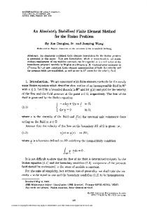
Figure 1: 𝐻1 -norm and 𝐿 2 -norm of errors for (46) with 𝛼 = 0.9, 𝛽 = 0.5, Δ𝑥 = 0.001 (a), and Δ𝑡 = 0.001 (b).

−8 −9 −10

−4 −5 −6

−11

−7

−12

−8

−13 −5

−4.5

−4

−3.5 −3 Δ𝑡 in logscale

−2.5

−2

𝐻1 -norm 𝐿 2 -norm

−9 −5

−4.5

−4

−3 −3.5 Δ𝑥 in logscale

−2.5

−2

𝐻1 -norm 𝐿 2 -norm (a)

(b)

Figure 2: 𝐻1 -norm and 𝐿 2 -norm of errors for (46) with 𝛼 = 0.5, 𝛽 = 0.25, Δ𝑥 = 0.001 (a), and Δ𝑡 = 0.001 (b).

where the right-side function 𝑓(𝑡, 𝑥) = (2𝑡2−𝛼 /Γ(3 − 𝛼)) sin(2𝜋𝑥)+(2𝑡2−𝛽 /Γ(3−𝛽)) sin(2𝜋𝑥)+4𝜋2 sin(2𝜋𝑥)𝑡2 . The exact solution is 𝑢(𝑡, 𝑥) = 𝑡2 sin(2𝜋𝑥). We use this example to check the convergence rate (c. rate) and CPU time (CPUT) of numerical solutions with respect to the fractional orders 𝛼 and 𝛽. In the first test, we fix 𝑇 = 1, 𝛼 = 0.9 and 𝛽 = 0.5 and choose Δ𝑥 = 0.001 which is small enough such that the space discretization errors are negligible as compared with the time errors. Choosing Δ𝑡 = 1/2𝑖 (𝑖 = 2, 4, . . . , 7), we report that the convergence rate of FDM in time is nearly 1.15 in Table 1, which matches well with the result of Theorem 4. On the

other hand, Table 2 shows that an approximate convergence rate is 2, by fixing Δ𝑡 = 0.001 and choosing Δ𝑥 = 1/2𝑖 (𝑖 = 2, . . . , 6), which matches well with the result of Theorem 6. In the second test, we give the convergence rate when 𝛼 = 0.5, 𝛽 = 0.25 for Δ𝑡 in Table 3, and Δ𝑥 in Table 4, respectively. We also report the 𝐿 2 -norm and 𝐻1 -norm of errors in Figures 1 and 2, respectively. Fixing Δ𝑥 = 0.001, 𝛼 = 0.9, and 𝛽 = 0.3 in (46), we compare the error and CPUT calculated by the FEM in this paper with the FDM in [8] and the FPCM in [8]. From Table 5, it can be seen that the FEM in this paper is computationally effective.

8

Abstract and Applied Analysis Table 1: Convergence rate in time for (46) with 𝛼 = 0.9 and 𝛽 = 0.5.

Δ𝑥 0.001 0.001 0.001 0.001 0.001

𝐻1 -norm 1.3815 × 10−2 6.1890 × 10−3 2.7858 × 10−3 1.2571 × 10−3 5.6567 × 10−4

Δ𝑡 1/4 1/16 1/32 1/64 1/128

𝐿 2 -norm 1.8960 × 10−3 8.4939 × 10−4 3.8234 × 10−4 1.7252 × 10−4 7.7635 × 10−5

c. rate

CPUT (seconds) 0.214 0.357 0.736 1.438 2.922

1.1585 1.1516 1.1481 1.1520

Table 2: Convergence rate in space for (46) with 𝛼 = 0.9 and 𝛽 = 0.5. Δ𝑡 0.001 0.001 0.001 0.001 0.001

𝐻1 -norm 0.2294 5.9763 × 10−2 1.5067 × 10−2 3.7356 × 10−3 8.9129 × 10−4

Δ𝑥 1/4 1/16 1/32 1/64 1/128

𝐿 2 -norm 3.0611 × 10−2 8.0381 × 10−3 2.0442 × 10−3 5.0966 × 10−4 1.2198 × 10−4

c. rate

CPUT (seconds) 20.35 21.85 26.68 32.72 41.03

1.9291 1.9753 2.0039 2.0629

Table 3: Convergence rate in time for (46) with 𝛼 = 0.5 and 𝛽 = 0.25. Δ𝑥 0.001 0.001 0.001 0.001 0.001

𝐻1 -norm 3.0985 × 10−3 1.0789 × 10−3 3.6702 × 10−4 1.1772 × 10−4 3.0704 × 10−5

Δ𝑡 1/4 1/16 1/32 1/64 1/128

𝐿 2 -norm 4.2525 × 10−4 1.4807 × 10−4 5.0372 × 10−5 1.6156 × 10−5 4.2139 × 10−6

c. rate

CPUT (seconds) 0.218 0.413 0.921 1.855 3.783

1.5221 1.5556 1.6406 1.6388

Table 4: Convergence rate in space for (46) with 𝛼 = 0.5 and 𝛽 = 0.25. Δ𝑡 0.001 0.001 0.001 0.001 0.001

𝐻1 -norm 2.3325 × 10−1 6.0836 × 10−2 1.5382 × 10−2 3.8569 × 10−3 9.6378 × 10−4

Δ𝑥 1/4 1/16 1/32 1/64 1/128

𝐿 2 -norm 3.1119 × 10−2 8.1823 × 10−3 2.0870 × 10−3 5.2622 × 10−4 1.3189 × 10−4

c. rate

CPUT (seconds) 23.73 26.29 33.49 41.68 55.24

1.9272 1.9711 1.9877 1.9963

Table 5: Comparison of error and CPUT for (46) with 𝛼 = 0.9 and 𝛽 = 0.3. Δ𝑥 0.001 0.001 0.001 0.001 0.001

Δ𝑡 1/4 1/8 1/16 1/32 1/64

FEM

FDM [8]

FPCM [8]

Error

CPUT

Error

CPUT

Error

CPUT

3.7056 × 10−3 1.6794 × 10−3 7.6528 × 10−4 3.5009 × 10−4 1.6027 × 10−4

0.238 0.481 0.962 1.335 2.703

5.8723 × 10−3 2.6751 × 10−3 1.2159 × 10−3 5.5190 × 10−4 2.4997 × 10−4

0.897 1.837 3.512 7.001 14.45

2.2027 × 10−2 8.7467 × 10−3 3.4693 × 10−3 1.3765 × 10−3 5.4564 × 10−4

6.16 16.63 30.11 52.71 106.49

Table 6: Comparison of error, convergence rate, and CPUT for (47) with 𝛼 = 0.5 and 𝛽 = 0.3. Δ𝑡

DFBDM (Section 3) Error

1/4

9.1975 × 10−4

1/8 1/16 1/32

3.3037 × 10−4 1.1375 × 10−4 3.5112 × 10−5

c. rate 1.4772 1.5382 1.6958

FEM2 [28] CPUT

Error

0.000864

3.6606 × 10−3

0.001986 0.004649 0.012112

7.8173 × 10−3 1.6210 × 10−4 3.2629 × 10−4

c. rate

CPUT 0.001862

2.2274 2.2697 2.3127

0.004902 0.051816 0.518130

Abstract and Applied Analysis

9

Example 10. Consider the following multierm fractional differential problem: 𝐶 𝛼 0 𝐷𝑡 𝑢 (𝑡)

𝛽

+ 𝑡−0.2 0𝐶𝐷𝑡 𝑢 (𝑡) = 𝑓 (𝑡) ,

𝑢 (0) = 0,

(47)

where 𝑓(𝑡) = (4𝑡1.5 /Γ(2.5)) + (12𝑡2 /Γ(3.5)). For 𝛼 = 0.5 and 𝛽 = 0.3, the exact solution is 𝑢(𝑡) = 𝑡2 + 𝑡2.5 . For the problem (47), our method in this paper is just the DFBDM in Section 3. Therefore, we only need to compare M1 with the FEM in [28] (FEM2). In Table 6, although the convergence rate of FEM2 is higher than that of DFBDM, the error and CPUT of DFBDM are smaller than those of FEM2.

Acknowledgments The authors are grateful to the referees for their valuable comments. This work is supported by the National Natural Science Foundation of China (11101109 and 11271102), the Natural Science Foundation of Hei-Long-Jiang Province of China (A201107), and SRF for ROCS, SEM.

References [1] C. Li, Z. Zhao, and Y. Chen, “Numerical approximation and error estimates of a time fractional order diffusion equation,” in Proceedings of the ASME International Design Engineering Technical Conference and Computers and Information in Engineering Conference (IDETC/CIE ’09), San Diego, Calif, USA, 2009. [2] Y. Jiang and J. Ma, “High-order finite element methods for timefractional partial differential equations,” Journal of Computational and Applied Mathematics, vol. 235, no. 11, pp. 3285–3290, 2011. [3] X. J. Li and C. J. Xu, “Existence and uniqueness of the weak solution of the space-time fractional diffusion equation and a spectral method approximation,” Communications in Computational Physics, vol. 8, no. 5, pp. 1016–1051, 2010. [4] K. Diethelm and N. J. Ford, “Numerical solution of the BagleyTorvik equation,” Numerical Mathematics, vol. 42, no. 3, pp. 490–507, 2002. [5] K. Diethelm and N. J. Ford, “Multi-order fractional differential equations and their numerical solution,” Applied Mathematics and Computation, vol. 154, no. 3, pp. 621–640, 2004. [6] V. Daftardar-Gejji and S. Bhalekar, “Boundary value problems for multi-term fractional differential equations,” Journal of Mathematical Analysis and Applications, vol. 345, no. 2, pp. 754– 765, 2008. [7] H. Jiang, F. Liu, I. Turner, and K. Burrage, “Analytical solutions for the multi-term time-space Caputo-Riesz fractional advection-diffusion equations on a finite domain,” Journal of Mathematical Analysis and Applications, vol. 389, no. 2, pp. 1117– 1127, 2012. [8] F. Liu, M. M. Meerschaert, R. J. McGough, P. Zhuang, and Q. Liu, “Numerical methods for solving the multi-term timefractional wave-diffusion equation,” Fractional Calculus and Applied Analysis, vol. 16, no. 1, pp. 9–25, 2013. [9] G. Psihoyios and T. E. Simos, “Trigonometrically fitted predictor-corrector methods for IVPs with oscillating solutions,” Journal of Computational and Applied Mathematics, vol. 158, no. 1, pp. 135–144, 2003.

[10] T. E. Simos, I. T. Famelis, and C. Tsitouras, “Zero dissipative, explicit Numerov-type methods for second order IVPs with oscillating solutions,” Numerical Algorithms, vol. 34, no. 1, pp. 27–40, 2003. [11] T. E. Simos, “Dissipative trigonometrically-fitted methods for linear second-order IVPs with oscillating solution,” Applied Mathematics Letters, vol. 17, no. 5, pp. 601–607, 2004. [12] G. Psihoyios and T. E. Simos, “A fourth algebraic order trigonometrically fitted predictor-corrector scheme for IVPs with oscillating solutions,” Journal of Computational and Applied Mathematics, vol. 175, no. 1, pp. 137–147, 2005. [13] S. Stavroyiannis and T. E. Simos, “Optimization as a function of the phase-lag order of nonlinear explicit two-step P.-stable method for linear periodic IVPs,” Applied Numerical Mathematics, vol. 59, no. 10, pp. 2467–2474, 2009. [14] G. A. Panopoulos and T. E. Simos, “An optimized symmetric 8-Step semi-embedded predictor-corrector method for IVPs with oscillating solutions,” Applied Mathematics & Information Sciences, vol. 7, no. 1, pp. 73–80, 2013. [15] A. Konguetsof and T. E. Simos, “A generator of hybrid symmetric four-step methods for the numerical solution of the Schr¨odinger equation,” Journal of Computational and Applied Mathematics, vol. 158, no. 1, pp. 93–106, 2003. [16] Z. Kalogiratou, Th. Monovasilis, and T. E. Simos, “Symplectic integrators for the numerical solution of the Schr¨odinger equation,” Journal of Computational and Applied Mathematics, vol. 158, no. 1, pp. 83–92, 2003. [17] D. P. Sakas and T. E. Simos, “Multiderivative methods of eighth algebraic order with minimal phase-lag for the numerical solution of the radial Schr¨odinger equation,” Journal of Computational and Applied Mathematics, vol. 175, no. 1, pp. 161–172, 2005. [18] T. E. Simos, “Exponentially and trigonometrically fitted methods for the solution of the Schr¨odinger equation,” Acta Applicandae Mathematicae, vol. 110, no. 3, pp. 1331–1352, 2010. [19] T. E. Simos, “Optimizing a hybrid two-step method for the numerical solution of the Schr¨odinger equation and related problems with respect to phase-lag,” Journal of Applied Mathematics, vol. 2012, Article ID 420387, 17 pages, 2012. [20] Z. A. Anastassi and T. E. Simos, “A parametric symmetric linear four-step method for the efficient integration of the Schr¨odinger equation and related oscillatory problems,” Journal of Computational and Applied Mathematics, vol. 236, no. 16, pp. 3880–3889, 2012. [21] K. Tselios and T. E. Simos, “Runge-Kutta methods with minimal dispersion and dissipation for problems arising from computational acoustics,” Journal of Computational and Applied Mathematics, vol. 175, no. 1, pp. 173–181, 2005. [22] Z. A. Anastassi and T. E. Simos, “An optimized Runge-Kutta method for the solution of orbital problems,” Journal of Computational and Applied Mathematics, vol. 175, no. 1, pp. 1–9, 2005. [23] D. F. Papadopoulos and T. E. Simos, “A modified RungeKutta-Nystr¨om method by using phase lag properties for the numerical solution of orbital problems,” Applied Mathematics & Information Sciences, vol. 7, no. 2, pp. 433–437, 2013. [24] T. Monovasilis, Z. Kalogiratou, and T. E. Simos, “Exponentially fitted symplectic Runge-Kutta-Nystr¨om methods,” Applied Mathematics & Information Sciences, vol. 7, no. 1, pp. 81–85, 2013. [25] Z. Kalogiratou and T. E. Simos, “Newton-Cotes formulae for long-time integration,” Journal of Computational and Applied Mathematics, vol. 158, no. 1, pp. 75–82, 2003.

10 [26] T. E. Simos, “Closed Newton-Cotes trigonometrically-fitted formulae of high order for long-time integration of orbital problems,” Applied Mathematics Letters, vol. 22, no. 10, pp. 1616– 1621, 2009. [27] T. E. Simos, “New stable closed Newton-Cotes trigonometrically fitted formulae for long-time integration,” Abstract and Applied Analysis, vol. 2012, Article ID 182536, 15 pages, 2012. [28] A. A. Badr, “Finite element method for linear multiterm fractional differential equations,” Journal of Applied Mathematics, vol. 2012, Article ID 482890, 9 pages, 2012. [29] N. J. Ford, J. Xiao, and Y. Yan, “A finite element method for time fractional partial differential equations,” Fractional Calculus and Applied Analysis, vol. 14, no. 3, pp. 454–474, 2011. [30] I. Podlubny, Fractional Differential Equations, vol. 198, Academic Press, San Diego, Calif, USA, 1999. [31] S. G. Samko, A. A. Kilbas, and O. I. Marichev, Fractional Integrals and Derivatives: Theory and Applications, Gordon and Breach Science, Philadelphia, Pa, USA, 1993. [32] X. J. Li and C. J. Xu, “A space-time spectral method for the time fractional diffusion equation,” SIAM Journal on Numerical Analysis, vol. 47, no. 3, pp. 2108–2131, 2009. [33] K. Diethelm, “An algorithm for the numerical solution of differential equations of fractional order,” Electronic Transactions on Numerical Analysis, vol. 5, no. 1, pp. 1–6, 1997. [34] K. Diethelm, “Generalized compound quadrature formulae for finite-part integrals,” IMA Journal of Numerical Analysis, vol. 17, no. 3, pp. 479–493, 1997. [35] V. Thom´ee, Galerkin Finite Element Methods for Parabolic Problems, Springer, Berlin, Germany, 2006.

Abstract and Applied Analysis

Advances in

Operations Research Hindawi Publishing Corporation http://www.hindawi.com

Volume 2014

Advances in

Decision Sciences Hindawi Publishing Corporation http://www.hindawi.com

Volume 2014

Journal of

Applied Mathematics

Algebra

Hindawi Publishing Corporation http://www.hindawi.com

Hindawi Publishing Corporation http://www.hindawi.com

Volume 2014

Journal of

Probability and Statistics Volume 2014

The Scientific World Journal Hindawi Publishing Corporation http://www.hindawi.com

Hindawi Publishing Corporation http://www.hindawi.com

Volume 2014

International Journal of

Differential Equations Hindawi Publishing Corporation http://www.hindawi.com

Volume 2014

Volume 2014

Submit your manuscripts at http://www.hindawi.com International Journal of

Advances in

Combinatorics Hindawi Publishing Corporation http://www.hindawi.com

Mathematical Physics Hindawi Publishing Corporation http://www.hindawi.com

Volume 2014

Journal of

Complex Analysis Hindawi Publishing Corporation http://www.hindawi.com

Volume 2014

International Journal of Mathematics and Mathematical Sciences

Mathematical Problems in Engineering

Journal of

Mathematics Hindawi Publishing Corporation http://www.hindawi.com

Volume 2014

Hindawi Publishing Corporation http://www.hindawi.com

Volume 2014

Volume 2014

Hindawi Publishing Corporation http://www.hindawi.com

Volume 2014

Discrete Mathematics

Journal of

Volume 2014

Hindawi Publishing Corporation http://www.hindawi.com

Discrete Dynamics in Nature and Society

Journal of

Function Spaces Hindawi Publishing Corporation http://www.hindawi.com

Abstract and Applied Analysis

Volume 2014

Hindawi Publishing Corporation http://www.hindawi.com

Volume 2014

Hindawi Publishing Corporation http://www.hindawi.com

Volume 2014

International Journal of

Journal of

Stochastic Analysis

Optimization

Hindawi Publishing Corporation http://www.hindawi.com

Hindawi Publishing Corporation http://www.hindawi.com

Volume 2014

Volume 2014