Stability and Instability of a Two-Station Queueing Network

Stability and Instability of a Two-Station Queueing Network J. G. Dai1 School of Industrial and Systems Engineering and School of Mathematics, Georgia Institute of Technology, Atlanta, GA 30332-0205, USA [email protected] John J. Hasenbein2 Graduate Program in Operations Research and Industrial Engineering, Department of Mechanical Engineering, University of Texas at Austin, Austin, TX 78712-1063, USA [email protected] John H. Vande Vate3 School of Industrial and Systems Engineering, Georgia Institute of Technology, Atlanta, GA 30332-0205, USA [email protected] Abstract This paper proves that the stability region of a 2-station, 5-class reentrant queueing network, operating under a non-preemptive static buffer priority service policy, depends on the distributions of the interarrival and service times. In particular, our result shows that conditions on the mean interarrival and service times are not enough to determine the stability of a queueing network, under a particular policy. We prove that when all distributions are exponential, the network is unstable in the sense that, with probability one, the total number of jobs in the network goes to infinity with time. We show that the same network with all interarrival and service times being deterministic is stable. When all distributions are uniform with a given range, our simulation studies show that the stability of the network depends on the width of the uniform distribution. Finally, we show that the same network, with deterministic interarrival and service times, is unstable when the it is operated under the preemptive version of the static buffer priority service policy. Thus, our examples also demonstrate that the stability region depends on the preemption mechanism used.

Keywords: multiclass queueing network, reentrant line, stability, fluid model, virtual station, push start, large deviations estimate June 1, 2001

1

Introduction

This paper is part of an ongoing effort to understand the relationship between the stability of a queueing network and the stability of the corresponding fluid model; see Rybko and Stolyar [27], Dai [8], Stolyar [29], Dai and Meyn [11], Chen [6], Meyn [25], Dai [10], Bramson [4, 5] and Pulhaskii and Rybko [26]. The fluid model is a continuous, deterministic analog of a discrete stochastic queueing network, and is defined through a set of equations. It is known that the stability of a queueing network is implied by the stability of its fluid model; the stability analysis of the latter, 1 Research supported in part by NSF grants DMI-94-57336 and DMI-9813345 and by the Logistics Institute Asia Pacific (TLI-AP), a partnership between the National University of Singapore and the Georgia Institute of Technology. 2 Research supported in part by NSF grant INT-9971484. 3 Research supported in part by NSF grant DMI-9813345.

1

though still nontrivial, is often significantly easier than the former; see, for example [1, 3, 7, 13, 20, 23]. Recently, Bramson [5] gave an example of a queueing network that is stable, but whose fluid model is not stable. The queueing network studied in this paper has 2 service stations and 5 job classes. It belongs to a special class of networks called reentrant lines by Kumar [22]. The network is assumed to be operating under a non-preemptive static buffer priority (SBP) service policy, and to have fixed mean interarrival and service times. We first consider a model in which all interarrival and service time distributions are assumed to be deterministic. Theorem 2.1 posits that the deterministic network is stable. We next analyze the network under the assumption that all interarrival and service time distributions are exponential. In Theorem 2.2, we prove that such a queueing network is unstable in the sense that, with probability 1, the total number of jobs in the system goes to infinity with time. A consequence of Theorems 2.1 and 2.2 is that the stability region of the 2-station queueing network depends on the distributions, not just the means, of the interarrival and service times. For queueing networks operating under a head-of-line (HOL) service policy, practical fluid models are defined through a set of equations, known as the fluid model equations, which take the mean interarrival and service times as parameters. Hence, a further consequence of our result is that no mean-value based fluid model can determine the stability of the queueing network we study. For a queueing network operating under a given service policy, each fluid model equation in the corresponding fluid model can be added only when it can be justified by a limiting procedure via fluid limits; see, for example, Section 7 of Dai [8]. Some equations, like the ones balancing the flows among job classes, can be derived and justified easily. Others, in particular those that are specific to a service policy, are more difficult to divine and justify. Generating and verifying such fluid model equations sometimes requires great insight and deep analysis of the queueing network itself; see, for example, the virtual station fluid model equations (14)–(16) in Dai and Vande Vate [13]. Nevertheless, this add hoc way of writing down fluid model equations have been quite successful because it is practical and works well for a number for service policies. For Bramson’s example in [5], one may wonder if, by adding additional fluid model equations, a modified fluid model would be stable, thus nullifying the result in [5]. Such a scenario, while unlikely, was not ruled out in Bramson’s paper. As noted above, our main result precludes the possibility that adding more fluid equations could ever result in a complete mean-value fluid model for the network we consider. In Dai and Vande Vate [13], it was shown that 2-station multitype fluid models are globally stable (i.e., stable under any non-idling service policy) if and only if the virtual station and push start conditions are satisfied. (See Section 10 for further discussion of these conditions.) In conjunction with the stability result in Dai [8], this implies that the virtual station and push start conditions are sufficient for global stability of 2-station multitype queueing networks, with general interarrival and service distributions. The next natural question which arises is whether these conditions are also necessary for the stability of such queueing networks. If so, then the fluid model can be used to completely characterize the global stability of this class of queueing networks. A pathwise argument (see, e.g. [12] and [19]) can be used to demonstrate that virtual station conditions are indeed necessary for the global stability of networks with general interarrival and service distributions. The queueing network considered in this paper provides a test case for determining the necessity of push start conditions. For the exponential queueing network, Dai and Vande Vate’s virtual station condition is satisfied. However, the push start condition is violated. Theorem 2.2 indicates that the push start condition is indeed also necessary for global stability of the exponential queueing network. We believe that it is likely that such a principle holds for all 2-station multitype queueing networks with exponential distributions, i.e., in such networks the virtual station and push start conditions completely characterize the global stability region. We anticipate that the proof techniques used 2

here will be of use in establishing a more general result of this type. The discussion so far in this section has assumed that the SBP service policy is non-preemptive. In Theorem 2.3, however, we give a result for the deterministic network operating under the preemptive SBP service policy. In particular, we show that the network is unstable when operated under the preemptive SBP policy, while Theorem 2.1 proves that the same network operating under the non-preemptive SBP policy is stable. Our finding contrasts a common brief that the preemption mechanism should have little effect on system performance measures like throughput and cycle time, at least when the system is heavily loaded [17]. Indeed, Williams [31] shows that the heavy traffic behavior under any HOL service policy is insensitive to the preemption mechanism employed as long as a certain multiplicative state space collapse condition is satisfied. Our example suggests that the state space collapse condition itself may depend on the preemption mechanism used. To our knowledge, this paper is the first to demonstrate that the stability region of a standard multiclass queueing network operating under an HOL service policy depends on the distributions of interarrival and service times. The first paper which directly showed the gap between the stability of a multiclass queueing network and its fluid model was Bramson [5]. Other researchers have also investigated the relation between the stability of a queueing model and its corresponding fluid model (or the corresponding family of fluid limits). Foss and Kovalevskii [16] consider a polling model and show that the standard definition of stability of a fluid model (see [8], [29]) does not suffice in order to characterize the stability of their stochastic polling model. They present a refined definition of fluid stability which captures the stability behavior of the original system. Stolyar and Ramakrishnan [30] investigate the stability of another type of polling model which falls outside the scope of the standard multiclass queueing network. They also demonstrate that the standard criterion for defining the stability of fluid limits does not properly characterize the stability of the original model. Again, a more refined fluid stability criterion is introduced which characterizes the fluid behavior in a more satisfactory manner. Essentially, both papers propose a more careful examination of the fluid limit model rather than the fluid model. The fluid model is a deterministic, mean-value based model, whereas the fluid limit model considers only the (possibly stochastic) weak limits of the rescaled queue-length process. Although it is possible that investigating fluid limits directly could result in a tight characterization of the stability for a general multiclass network, it is unclear if this approach will be of practical use. The main difficulty is that characterizing the stability of a fluid limit model could be as intractable as characterizing the stability of the original model. Heretofore, the primary appeal of the fluid model has been the relative simplicity of stability analysis. The rest of paper is organized as follows. In Section 2, we introduce the 2-station queueing network, and state our main results. In Section 3, we introduce the fluid model which corresponds to the queueing network described in Section 2. In this section we also present a stable fluid solution which drains and an unstable fluid solution that diverges to infinity, where both solutions have the same initial state. Section 4 presents the proof of Theorem 2.1, regarding the deterministic network. Sections 5 and 6, which occupy a large portion of the paper, are devoted to the proof of Theorem 2.2. For the casual reader, these two sections can be skipped. In Section 7 we present some simulation results which explore the stability behavior of the uniform network. Section 8 contains the proof of Theorem 2.3 and Section 9 gives a proof outline of a result that is analogous to Theorem 2.2, when the exponential network is operated under the preemptive SBP service policy. Finally, in Section 10, we present a more detailed discussion of virtual station and push start conditions. We end the paper with an appendix in which details of some proofs are presented.

3

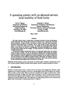
α1 = 1

-

m1 = 0.4

m3 = 0.4

-

¾

m2 = 0.1

-

m4 = 0.1

¾

-

m5 = 0.4

Station B

Station A

Figure 1: A Push Started Lu-Kumar Network

2

The Queueing Network Model and Main Results

In this section, we first define the queueing network model to be studied in this paper. We then state our main results.

2.1

The queueing network model

In this paper we will only be concerned with the queueing network pictured in Figure 1. The network has 2 service stations, each having a single server. Each job follows the deterministic route indicated in the figure, making a total of 5 visits along the route. Each station may only serve one job at any given time. Jobs that are in service or waiting for the kth step of service are called class k jobs. We envision them waiting in buffer k in front of the station. With a slight abuse of notation, we consider a class k job that is in service also belongs to buffer k. We assume that the service times for class k jobs are i.i.d. random variables with mean mk , k = 1, . . . , 5. The interarrival times for jobs arriving from the outside are also assumed to be i.i.d. random variables with mean 1/α1 . Thus, α1 is the exogenous arrival rate. We further assume that the sequence of interarrival times and the 5 sequences of service times are mutually independent. Throughout this paper, unless explicitly specified otherwise, we fix the arrival rate and mean service times to be α1 = 1,

m1 = 0.4,

m2 = 0.1,

m3 = 0.4,

m4 = 0.1 and

m5 = 0.4.

(1)

In this paper, we consider several variations of the general network described above. In all cases, the interarrival time distribution and five service time distributions are assumed to all have the same type of distribution, either deterministic, exponential, or uniform. We will refer to the associated network as either the deterministic network, the exponential network, or the uniform network, respectively. Since we have fixed the mean interarrival and service times, in the deterministic case, the means completely define the respective distributions. In the exponential network, all intearrival and service time distributions are assumed to be exponential with mean values as specified above. For a uniform network, to specify the distributions we need to specify the supports of these uniform distributions. Each uniform distribution is centered at the mean values above, with a width of ². For ease of exposition, we assume that the widths for the interarrival and the five service time

4

distributions are all the same. Thus, for the uniform networks we discuss, we can fully specify the distributions with the parameter ², since the mean values are fixed. Now we discuss the service policy to be employed in the network under study. When either Station A or B completes the service of a job, it must determine which job to pick next for service. A service (or dispatch) policy specifies how each station makes this decision for every possible state of the network. Our network is assumed to be operating under the non-idling static buffer priority (SBP) service policy π = {(1, 3, 4), (5, 2)}. Under this policy, at Station A jobs of class 1 have highest priority, class 3 jobs have second highest priority, and class 4 jobs are given lowest priority. At Station B, class 5 jobs have high priority and class 2 jobs have low priority. We can consider both non-preemptive and preemptive versions of the policy π. Under a non-preemptive service policy, once a job is in service, this job must be completed before its server can serve any other jobs. Under a preemptive service policy, a job in service can be preempted by an arriving higher priority job. The preempted job is then served from where it left off when the server completes all higher priority jobs. We primarily consider the non-preemptive service policy. However, in Sections 8 and 9 we give some results on the network operating under the preemptive policy. We use Zk (t) to denote the number of jobs in buffer k at time t and Z(t) = (Z1 (t), . . . , Z5 (t)) to denote the corresponding vector. We use |Z(t)| to denote the total number of jobs in the network at time t. For the exponential network the vector Z(t) completely determines the state of the system in the preemptive case. Namely, if one knows Z(t) at time t, the future evolution of the network can be determined from time t on. For the deterministic or uniform networks, the state Z(t) is not sufficient to determine the future evolution of the network. One also needs to know the remaining interarrival and service times at t to completely specify the state of the system. Furthermore, in the non-preemptive case, one must also specify which job is currently in service, no matter what distributional assumption is in effect. In later sections, we will sometimes augment the buffer level state Z(t) with additional information needed to fully specify the network state.

2.2

Main results

Here we present the main theoretical results and also summarize some of our simulation results. The first result shows that, under the non-preemptive SBP service policy the deterministic network is stable (from all initial states). The second result shows that the number of jobs in the exponential network diverges to infinity, from any initial state. Finally, we show that the deterministic network operating under the preemptive SBP policy is unstable from at least one class of states. The first two results show that changing the distribution for the interarrival and service times has a profound effect on network dynamics. The first and third results demonstrate that changing the preemption mechanism also has a dramatic effect. Finally, our simulation results indicate that simply changing the range of the distributions in a uniform network also affects the stability of the network. We now state the main results more precisely. The first theorem concerns the deterministic network operating under the non-preemptive SBP service policy. In the deterministic network, a fully specified system state should indicate the number of jobs in each class, which classes of jobs are in service, the remaining time until the next job arrives, and the remaining service times for all jobs in service. For notational convenience, we use some subset of this information to define a “special state” (z1 , z2 , z3 , z4 , z5 ; a), where zk is the number of jobs in buffer k and a is the remaining interarrival time until the next job arrives to the network. These special states, observed at service completion times, indeed indicate the complete system state due to the deterministic evolution of the network. With a slight abuse of terminology, such special states are simply called states.

5

In Lemma 4.1 we verify that for any 0 < a ≤ 0.1 when the deterministic network starts in state (0, 0, 0, 1, 0; a), the network will come back to this same state exactly one minute later. Thus, the trajectory starting from state (0, 0, 0, 1, 0; a) forms an orbit. For a given 0 < a ≤ 0.1, the corresponding orbit is called an a-orbit. With this definition in hand, we now state our first result. Theorem 2.1. For the deterministic network operating under the non-preemptive priority SBP service policy, starting from any state, there exists a finite time at which the network enters an a-orbit, with 0 < a ≤ 0.1. As we demonstrate later, while in an a-orbit, the network has at most two jobs. Hence, a consequence of Theorem 2.1 is that the total number of jobs in the deterministic network is at most 2 after some finite time (which depends on the initial state). The next theorem shows that the number of jobs in the exponential network diverges to infinity. Theorem 2.2. For the exponential network operating under the non-preemptive SBP service policy, starting from any initial state, |Z(t)| → ∞ as t → ∞ with probability one. One can adopt a number of definitions of stability for a network. We do not adopt any specific definition in this paper, but present some different notions of stability in order to put our results in perspective. Definition 2.1. The 2-station queueing network is said to be stochastically bounded if starting from any initial state x, ½ ¾ lim Px lim sup |Z(t)| ≤ M = 1. M →∞

t→∞

For the exponential network, being stable in the stochastic boundedness sense is equivalent to the state process for the network being positive recurrent. For the deterministic network, stochastic boundedness is equivalent to the recurrence property of the trajectory. Hence, if we adopt stochastic bounedness as the definition for stability, then Theorem 2.1 and Theorem 2.2 show that the exponential network operating under the non-preemptive SBP policy is unstable while the deterministic network operating under the same policy is stable. Definition 2.2. The 2-station queueing network is said to be rate stable if starting from any initial state x, o n Px lim D5 (t)/t = α1 = 1, t→∞

where D5 (t) is the number of jobs which have departed the network in [0, t].

Although it is not proved in this paper, we suspect that Theorem 2.2 can be strengthened to show that, with probability one, the number of jobs in the network grows linearly with time. Such a result would imply that the exponential network is not rate stable, whereas Theorem 2.1 implies that the deterministic network is rate stable. The interested reader should refer to Chen [6] or El-Taha and Stidham [15] for more discussion on rate stability. Since the deterministic network is an extreme case where there is no randomness at all in the system, one may wonder if the fact that the stability of the network depends on the interarrival 6

and service distributions is a robust phenomenon or simply a pathological result which relies on the special deterministic case. In Section 7, we provide some simulation studies which indicate that the uniform network is stable for ² = 0.001 and unstable for ² = 0.1. Our final theorem implies that by allowing preemption in our SBP service policy, the deterministic network becomes unstable. Theorem 2.3. For the deterministic network operating under the preemptive SBP service policy, the number of jobs in the system grows linearly to infinity with time for any initial state Z(0) = (0, 0, 0, n, 0) for n sufficiently large. This theorem implies that the deterministic network operating under the preemptive policy is unstable, in both the stochastic boundedness and rate stable sense. So this result, along with Theorem 2.1, shows that the stability of the network depends on the preemption mechanism employed. Note that the exponential network is unstable, independent of the preemption mechanism employed (see Theorem 9.1, along with Theorem 2.2 from above).

3

Fluid model solutions

In this section we introduce the fluid model of our queueing network. The fluid model is especially important for our results since fluid model solutions give insight into the behavior of the networks we study. In addition to defining the fluid model below, we present both a stable and unstable fluid solution to the model. It turns out that the stable fluid solution and the stable trajectories of the deterministic network have the same qualitative behavior. Also, the proof of Theorem 2.2, given in Sections 5 and 6, is related to the unstable fluid solution. Essentially, the main idea of the proof, is to show that the exponential queueing network dynamics closely follow this unstable fluid model solution. The fluid model is a deterministic, continuous analog of the queueing network. It is defined through the following set of equations: Z1 (t) = Z1 (0) + α1 t − µ1 T1 (t),

t ≥ 0,

Zk (t) = Zk (0) + µk−1 Tk−1 (t) − µk Tk (t),

Zk (t) ≥ 0,

t ≥ 0,

k = 1, . . . , 5,

Tk (t) is non-decreasing in t,

(2) t ≥ 0,

k = 2, . . . , 5,

k = 1, . . . , 5,

Tk+ (t)

t− is non-decreasing in t, k = 1, . . . , 5, + T˙ (t) = 1 for any time t with Z + (t) > 0 for k = 1, . . . , 5, k

k

(3) (4) (5) (6) (7)

where, µk = 1/mk , Zk+ (t) is the sum of Z` (t) over all classes ` that have priority at least k and are served at the same station as class k. For example, for our network, operating under the priority policy defined in Section 2, we have Z4+ (t) = Z1 (t) + Z3 (t) + Z4 (t) and

Z1+ (t) = Z1 (t).

The quantity Tk+ (t) is defined in a similar manner. For a function f (·) : [0, ∞) → Rd for some integer d, f˙(t) denotes the derivative of f at time t. Each function (T, Z) satisfying (2)-(7) with T (t) = (T1 (t), . . . , T5 (t)) and Z(t) = (Z1 (t), . . ., Z5 (t)) is called a fluid solution to the fluid model. The quantities Z(t) and T (t) have the following interpretation. For each class k, Zk (t) is the fluid level in buffer k at time t, and Tk (t) is the 7

amount of time that the class k server has spent serving class k fluid in [0, t]. Thus, µ k Tk (t) is the cumulative amount of fluid that has departed from buffer k in [0, t]. Equations (2) and (3) simply balance the flows in the network. Equation (5) ensures that the amount of time spent on a class is non-decreasing and equation (6) says that the cumulative remaining time for a server, excluding the time spent on classes with priorities of at least k, is non-decreasing. Condition (7) follows from the SBP policies employed, i.e., when a high priority buffer has a positive amount of fluid, that server should not devote any effort to a lower priority buffer. In the cases k = 4 and k = 2, (7) simply insures that the fluid network operates under a non-idling policy. It can be shown that each fluid solution (T, Z) is Lipschitz continuous with respect to t; see, for example, Dai [9]. Therefore, each solution is also absolutely continuous and thus has derivatives for almost every t. Whenever a derivative like the one in (7) is employed, it is automatically assumed that (T, Z) is differentiable at time t. We construct two different fluid solutions, one which drains and one which diverges to infinity, from the same initial state. These two drastically different fluid solutions may give some insight as to why two queueing networks with the same fluid model may also have drastically different behavior. A stable fluid solution. We first construct a fluid solution that drains from the initial state Z(0) = (0, 0, 0, 1, 0), i.e. for this solution we have that Z(t) = 0 for all t > T , with T < ∞. In fact, this initial state is not special, nor is the specific set of network parameters we are using. It can be shown that as long as the usual traffic conditions: ρA := α1 (m1 + m3 + m4 ) < 1 and

ρB := α1 (m2 + m5 ) < 1,

(8)

hold, then we can similarly construct a stable fluid solution from any initial state. If one of the usual traffic conditions is violated, then no stable fluid solution exists, from any initial fluid state. To construct the stable fluid solution, we start the system with initial fluid level Z(0) = (0, 0, 0, 1, 0). The solution is qualitatively divided into two periods. During the first period, the network drains fluid from buffer 4, and does not accumulate fluid in any other buffers. Once the fluid is drained from buffer 4 at time t1 , the network can maintain all buffers empty from t1 on, which is the second part of the fluid solution. We use dk (t) to denote the departure rate µk T˙k (t) from class k at time t. Note that if we fully specify the departure rates dk (t), for t ≥ 0 and k = 1, . . . , 5 and for all t, a resulting fluid solution (T, Z) is uniquely defined. One needs to check that the solution satisfies the fluid model equations (2)-(7). In the case of our solution, this is relatively easy to verify. So, we first consider the time interval [0, 1). For t ∈ (0, 1) we set d1 (t) = d2 (t) = d3 (t) = 1 and

d4 (t) = d5 (t) = 2.

Since, under this set of departure rates, it is clear that only Z4 (t) is positive on [0, 1), we only need to check (7) for k = 4. One can check that for k = 4, (7) is equivalent to m1 d1 (t) + m3 d3 (t) + m4 d4 (t) = 1,

(9)

which clearly holds for the departure rates we have specified. To validity of (6) follows from (9) and the fact that m2 d2 (t) + m5 d5 (t) ≤ 1 holds for all t ∈ [0, 1) for the specified departure rates. The remainder of the fluid model equations are easily verified. 8

Under the departure rates given, it is clear that buffer 4 will empty at time t 1 = 1, with all other buffers remaining empty. So, at t1 , we have Z(t1 ) = (0, 0, 0, 0, 0). Next, on the interval (t1 , ∞) we set dk (t) = 1 for k = 1, . . . , 5, which yields Z(t) = (0, 0, 0, 0, 0) for t ∈ [t1 , ∞) Again, it is easy to check that (2)-(7) are satisfied for these departure rates and fluid buffer levels. Hence, we have demonstrated that there exists a stable fluid solution, starting from Z(0) = (0, 0, 0, 1, 0). An unstable fluid solution. Now we construct a fluid solution that diverges to infinity. Most of the proof of Theorem 2.2 is devoted to showing that, for the original exponential network, the network dynamics approximately follow this divergent fluid solution. As will be seen shortly, such a fluid solution exists because of the particular choices of the SBP policy and the mean service times employed in our network. It turns out that the divergent fluid solution always exists when the SBP policy is employed and the mean service times satisfy ρpush := α1 m5 + α1

m3 > 1. 1 − α 1 m1

(10)

When ρpush ≤ 1 and the usual traffic conditions hold, then no divergent fluid solution exists. Condition (10) violates the push start condition, first identified in Dai and Vande Vate [13]. The push start condition is a magnification of a virtual station phenomenon first observed by Harrison and Nguyen [18] and Dumas [14] and later systematically treated in Dai and Vande Vate [12] and [13]. See Section 10 for more discussion on virtual station and push start conditions. Now, to construct the divergent fluid solution, we start the system with initial fluid level Z(0) = (0, 0, 0, 1, 0). We present a fluid solution in one period that ends when the system state reaches a state (0, 0, 0, +, 0) with the fluid level in buffer 4 exceeding one unit. (The plus sign indicates the buffer level is positive.) Clearly, such a construction can be extended from period to period to construct a solution which diverges to infinity with time. Within a period, the system evolves in two cycles: the bottom cycle and the top cycle. During the bottom cycle, the initial fluid in buffer 4 drains into buffer 5 and then exits the network. During this draining period, fluid accumulates in buffer 2. The bottom cycle ends when all fluid has drained from buffers 4 and 5, and buffer 2 is the only buffer with a positive amount of fluid. At this point, the top cycle begins. During this cycle, fluid in buffer 2 drains into buffer 3 and accumulates in buffer 4. The cycle ends when all fluid has been drained from buffers 2 and 3 and all fluid in the network resides in buffer 4. The remainder of this section gives a detailed construction of these two cycles. We use d k (t) to denote the departure rate µk T˙k (t) from buffer k at time t. When the time t is clear from the context, we drop the time dependence from the departure rate notation. Note that if we fully specify the departure rates dk (t), for t ≥ 0 and k = 1, . . . , 5, a resulting fluid solution (T, Z) is uniquely defined. Of course, one needs to check that the solution satisfies the fluid model equations (2)-(7). This step is routine but tedious, and thus is not provided here. Bottom cycle. As the cycle begins, buffer 1 is initially empty. Since buffer 1 has highest priority, and the arrival rate to buffer 1 is slower than the service rate at buffer 1, buffer 1 will remain empty at all times. However, note that Station A needs to spend α1 m1 = 0.4 fraction of its time to keep buffer 1 empty. The remaining 60% of the server’s capacity may be spent on buffers 3 and 4. If Station A spends all of this 60% remaining capacity on buffer 4, it can process class 4 fluid at a rate of d4 = µ4 (1 − α1 m1 ) = 6, which is faster than the maximum service rate d5 = µ5 at buffer 5. Hence, at the beginning of the bottom cycle, class 4 fluid is being processed faster than class 5 fluid. So, fluid will accumulate at buffer 5 and furthermore, due to our priority policy, Station B 9

is prevented from serving any class 2 fluid. Therefore, for an initial period of time, buffers 1 and 3 remain empty with buffer 3 having no service activities at all, buffers 2 and 5 accumulate fluid, and buffer 4 drains fluid. Such a state will persist until buffer 4 empties at time t1 . At this point, the fluid level in the network is Z(t1 ) = (0, +, 0, 0, +), with a positive amount of fluid in buffers 2 and 5. Since there is no input to buffer 5 immediately after t1 , buffer 5 will begin draining fluid, and buffer 2 will continue to accumulate fluid. Meanwhile, all other buffers remain empty, with only buffers 1 and 5 processing fluid. This state will continue until buffer 5 empties at time t 2 . Note that during [0, t2 ), Station B is spending 100% of its effort processing class 5 fluid, and that it processes exactly one unit of fluid in this time. Hence, t2 = m5 and at this time, buffer 2 has α1 m5 units of fluid. Thus, the fluid level is given by Z(t2 ) = (0, α1 m5 , 0, 0, 0). This is the end of the bottom cycle. Top cycle. As soon as buffer 5 is empties, Station B begins processing class 2 fluid at rate d2 = µ2 = 10. This departure rate from buffer 2 will overwhelm buffer 3, which has a maximum service rate of µ3 = 2.5. Station A must continue to devote 40% of its time to class 1 fluid. Hence, Station A can only devote 60% of its capacity to buffer 3, and the departure rate from buffer 3 will be d3 = µ3 (1 − α1 m1 ) = 1.5. Furthermore, Station A cannot devote any processing capacity to class 4 fluid. Thus, in the period immediately after t2 , buffers 3 and 4 accumulate fluid, buffer 2 drains, and buffers 1 and 5 remain empty. This state will continue until buffer 2 empties at t 3 . From this point on, external fluid flows through buffers 1 and 2 instantaneously to buffer 3. Since this external rate α1 = 1 < d3 = 1.5, in the period immediately after t3 , class 3 fluid drains into buffer 4, buffer 4 accumulates fluid, and all other buffers remain empty. This state continues until buffer 3 empties at time t4 . At this time, all buffers are empty except buffer 4. Thus, the fluid level is Z(t4 ) = (0, 0, 0, +, 0). To calculate the amount of fluid in buffer 4, we note that the α 1 m5 units of fluid which were present in buffer 2 at time t2 have simply moved to buffer 4 at time t4 . In addition, α1 (t4 − t2 ) units of fluid have arrived from the outside during [t2 , t4 ] and reside in buffer 4 at t4 . Thus, Z4 (t4 ) = α1 m5 + α1 (t4 − t2 ). To calculate t4 − t2 , we note that during [t2 , t4 ], the departure rate from the “pipe” from buffer 1 to buffer 3 is a constant, d 3 . The input rate to this pipe is α1 . The initial amount in the pipe at t2 is α1 m5 . Thus, the pipe must empty in time t4 − t 2 =

α1 m 5 α1 m 5 m 3 m5 m3 = = . (d3 − α1 ) (1 − α1 m1 − α1 m3 ) (1 − m1 − m3 )

Hence, Z4 (t4 ) = α1 m5 + α1 (t4 − t2 ) =

α1 m 5 (1 − m1 )m5 6 = = > 1. 1 − α1 m3 /(1 − α1 m1 ) 1 − m 1 − m3 5

(11)

Therefore, our top cycle ends at time t4 with fluid level (0, 0, 0, 6/5, 0). One can check that in (11), Z4 (t4 ) > 1 is equivalent ρpush > 1, for general mean service times. Whenever the usual traffic conditions hold and ρpush > 1, our construction always leads to a divergent fluid solution.

4

The Deterministic Network with Non-preemption

In this section, we prove Theorem 2.1. Recall that the network has deterministic interarrival and service times, and is operated under the non-preemptive SBP service policy. Our first lemma justifies our earlier definition of an a-orbit. Lemma 4.1. Starting from an initial state (0, 0, 0, 1, 0; a) with 0 < a ≤ 0.1, the trajectory of the network returns to the same state one minute later. 10

Proof. The proof follows from simply examining the sequence of states the network visits in the first minute: Time 0 a 0.1 0.5 0.6 1.0

(0, (1, (1, (0, (0, (0,

0, 0, 0, 1, 0, 0,

State 0, 1, 0; 0, 1, 0; 0, 0, 1; 0, 0, 0; 1, 0, 0; 0, 1, 0;

a) 1) a+0.9) a+0.5) a+0.4) a).

Theorem 2.1 asserts that the network enters an a-orbit from any initial state. We first prove the theorem for initial states that are regular type 1 or type 2 states, which will be defined shortly. We then prove that the network, starting from any initial state, will eventually reach a regular state that is either of type 1 or type 2, thus proving the main theorem. Definition 4.1. 1. A regular state is a state which is reachable after the network has been in operation for at least one minute. 2. A type 1 state is any state of the form (0, 0, 0, n, 0; a) with n ≥ 0 and 0 < a ≤ 1. 3. A type 2 state is any state of the form (0, 1, 0, n, 0; a) with n ≥ 0 and 0 < a ≤ 1. Using Definition 4.1, it is easy to check that the following result holds. Lemma 4.2. 1. For a regular type 1 state, n ≥ 1 and 0 < a ≤ 0.1. 2. For a regular type 2 state, 0 < a ≤ 0.6. Without of loss of generality, we assume from now on that all initial states must be regular. Our first lemma shows that if the network starts from a regular type 1 state it will enter an a-orbit in a very direct manner. Note that if the network starts from any of the intermediate states in the proof of Lemma 4.3, it will enter an a-orbit. Lemma 4.3. Starting from a regular type 1 state, the network enters an a-orbit in (n − 1) minutes. Proof. For n = 1, the proof follows from our definition of an a-orbit. For n ≥ 2, the proof follows by observation of the following sequence of states and induction. Time 0 a 0.1 0.5 0.6 1.0

(0, (1, (1, (0, (0, (0,

0, 0, 0, 1, 0, 0,

0, 0, 0, 0, 1, 0,

11

State n, 0; a) n, 0; 1) n-1, 1; a+0.9) n-1, 0; a+0.5) n-2, 1; a+0.4) n-1, 0; a).

The next lemma indicates what occurs when the network starts from a regular type 2 state. Lemma 4.4. Starting from any regular type 2 state, the network eventually enters an a-orbit. The proof of Lemma 4.4 is left to the Appendix. Our final lemma in this section describes what happens from a general initial state. Note that such an initial state can be assumed to be regular, hence any subsequent state is also regular. Lemma 4.5. Starting from any (regular) initial state, the network eventually enters either a regular type 1 or regular type 2 state. Proof. First, we set r ≡ inf{t ≥ 0 : Z1 (t) = 0}, i.e. r is the first time that buffer 1 is empty. We claim that r is finite from any initial state and that Z1 (t) ≤ 1 for all t ≥ r. To see this, note that since class 1 jobs have highest priority and class 1 jobs are processed faster than the rate of arriving jobs, there will be some finite time at which Z1 (t) = 0. Next, after buffer 1 has drained for the first time, any class 1 arrival will begin processing no more than 0.4 minutes after its arrival (it may be delayed 0.4 minutes to wait for a class 3 job to complete processing). Since arrivals occur every minute, no more than one job can be in buffer 1 after it has drained for the first time. Now, set t1 ≡ inf{t ≥ r : Z2 (t)+Z5 (t) = 0}, i.e. t1 is the first time that Station B is empty, after buffer 1 has drained for the first time. By Lemma A.1 of the Appendix, t1 is finite. Furthermore, from our arguments above, we have Z(t1 ) = (1, 0, m, n, 0; a) or Z(t1 ) = (0, 0, m, n, 0; a), where m and n are arbitrary nonnegative integers and 0 < a ≤ 1. Note that the job in service at Station A may be in the middle of service at t1 . Next, to complete the proof, we examine the following cases. Case 1. A class 1 or class 3 job is in service at time t1 . In this case, no class 4 job can be processed until buffers 1 and 3 are both empty, due to our priority scheme. Let us denote by t2 the first time after t1 that a buffer 4 job enters service. Then immediately before t2 , Station A was serving either a class 1 or a class 3 job, both of which require 0.4 minutes of processing time. Note that no buffer 5 jobs are processed during [t 1 , t2 ], which implies that Z2 (t) ≤ 1, during this interval. If Station A was serving a class 3 job just before t 2 , then Z2 (t2 ) = 0 since there are no arrivals to buffer 2 during the 0.4 minute processing time of the class 3 job and class 2 jobs require only 0.1 minutes of processing time. Hence, in this case we must have Z(t2 ) = (0, 0, 0, n, 0, a), with n ≥ 1 and 0 < a ≤ 0.1, which is a regular type 1 state. If Station A was serving a class 1 job just before t2 , then we have Z(t2 ) = (0, 1, 0, n, 0; a). In order for Z(t2 ) to be a regular state, we must have 0 < a ≤ 0.6 at t2 . Thus in Case 1, the network will enter either a regular type 1 or type 2 state at t2 . Case 2. A class 4 job is in service at t1 and Z1 (t1 ) = Z3 (t1 ) = 0. First suppose that the class 4 job has just entered service. Then we must have Z(t1 ) = (0, 0, 0, n, 0; a) with n ≥ 1 and 0 < a ≤ 0.1, and we are in a regular type 1 state. If the class 4 job has a partial remaining service time at t1 , then at time t0 , when this job entered service, we have either Z(t0 ) = (0, 0, 0, n, 0; a) or Z(t0 ) = (0, 0, 0, n, 1; a) again with n ≥ 1 and 0 < a ≤ 0.1 in both cases. The former state is a regular type 1 state. In the latter case, the buffer 5 job must have less than 0.1 minutes partial remaining service time and one can check that the evolution of the network from such a state is the same as starting from a “pure” regular type 1 state. Case 3. A class 4 job is in service at t1 and Z1 (t1 ) = 1 or Z3 (t1 ) > 0 (or both). If Z1 (t1 ) = 1, then at t2 < t1 + 0.1 the class 4 job completes service and we have Z(t2 ) = (1, 0, m, n − 1, 1; a) with a > 0.9. At this time the class 1 and class 5 jobs will both initiate service. 0.4 minutes later, 12

the state is Z(t2 + 0.4) = (0, 1, m, n − 1, 0; a). If m = 0 the network is in a (regular) type 2 state. If m > 0 then 0.1 minutes later the class 2 job enters buffer 3, leaving Station B empty. In this case, the network is in a state of the form of Case 1, with a buffer 3 job in service. On the other hand, if Z1 (t1 ) = 0, then at t2 < t1 + 0.1 we have either Z(t2 ) = (1, 0, m, n − 1, 1; a) with a > 0.9 or Z(t2 ) = (0, 0, m, n − 1, 1; a) with m > 0. The former case has already been argued above. In the latter case, at t2 + 0.4 we will either be in a (regular) type 1 state (if there are no arrivals and m = 1) or we will be back in Case 1. Proof of Theorem 2.1. The proof of Theorem 2.1 now follows from the lemmas given in this section. Taking these lemmas together, we have that the network will enter an a-orbit from any initial state.

5

The Exponential Network – Preliminary Proofs

The majority of this section is devoted to proving the following theorem. Henceforth, we let t+ denote the time immediately after time t. Theorem 5.1. Consider the exponential network operating under the non-preemptive SBP service policy. Suppose Z(0) = (0, z2 , 0, n, z5 ) with a class 4 job entering service at time 0 and a class 2 job not in service at time 0+. Then for any 0 < θ < 1, there exists an ² > 0 such that for all sufficiently large n, ½ ¾ √ (1 − m1 )m5 P Z4 (T4 ) ≥ (12) θ n ≥ 1 − exp(−² n), 1 − m 1 − m3 where T2 = inf{t > 0 : Z3 (t) = Z4 (t) = Z5 (t) = 0},

(13)

T4 = inf{t > T2 : a class 4 job enters service at time t and a class 2 job is not in service at t+}.

(14)

Furthermore, for all sufficiently large n, P {|Z(t)| ≥ n/4,

∀t ∈ [0, T4 ]} ≥ 1 − exp(−²

√

n).

We envision n in the initial state Z(0) as large, with z2 and z5 being relatively small. However, the theorem holds for arbitrary z2 and z5 . Such an initial state corresponds to the initial fluid model state (0, 0, 0, 1, 0) used in Section 3. Note that at T4 , a class 4 job has just entered service. Thus it is necessarily true that buffers 1 and 3 are empty at T4 . Hence, at time T4 , the network has returned to a state similar to the initial state, with a magnification factor θ(1 − m 1 )m5 /(1 − m1 − m3 ). We will refer to the time interval [0, T4 ] as a cycle, in alignment with the fluid network dynamics. Similarly, the interval [0, T2 ] is said to form a bottom cycle and the interval [T2 , T4 ] is said to form a top cycle. The analogy between Theorem 5.1 and the unstable fluid solution constructed in Section 3 is evident. The magnification factor for the exponential network in (12) is smaller than the one for the fluid model in (11) due to randomness in our exponential network. However, since (1 − m1 )m5 /(1 − m1 − m3 ) > 1, one can always choose a θ < 1 such that the factor for the stochastic network in (12) is still strictly bigger than one. 13

Although we have said that our attention will be restricted to the network with a mean service time vector of m = (0.4, 0.1, 0.4, 0.1, 0.4), the proof of Theorem 5.1 is actually general and holds for any service time vector for which ρA < 1, ρB < 1 and ρpush > 1. In Section 6, we use Theorem 5.1 to complete the proof of Theorem 2.2. The remainder of this section is devoted to the proof of Theorem 5.1. The actual proof of Theorem 5.1 will be presented in Section 5.5, with the various lemmas presented in Sections 5.1–5.4. In Section 5.1, we show that during the bottom cycle the exponential network closely follows the unstable fluid solution in [0, t2 ]. In Section 5.3, we show that during the top cycle the exponential network closely follows the unstable fluid solution in [t2 , t4 ]. Sections 5.2 and 5.4 detail how the exponential network moves from the bottom cycle to the top cycle and from the top cycle to the bottom cycle, respectively. Readers who intend to read the rest of this section seriously should first understand thoroughly the unstable fluid solution constructed in Section 3. In the following sections, we will introduce a number of positive constants: ² 1 , ²2 , . . .. Since the exact values of the constants are not important for our final result, we will not keep track of the values or relationships between the constants.

5.1

The Bottom Cycle

At the beginning of what we call the bottom cycle, there are a large number of jobs in buffer 4. We wish to show that once these jobs begin processing, buffer 5 will eventually be overwhelmed with jobs, thus preventing buffer 2 jobs from being processed. Hence, once the large number of original class 4 jobs have completed processing at buffers 4 and 5, there will be a large build-up of jobs waiting at buffers 1 and 2. The goal of this subsection is show that with high probability, the behavior described above occurs and that the number of jobs in buffers 1 and 2 at the end of the bottom cycle is θ1 m5 n, where θ1 is a constant arbitrarily close to 1. These statements are made more precise in the following theorem, which is the main result for the bottom cycle. Theorem 5.2. Suppose Z(0) = (0, z2 , 0, n, z5 ) with a class 4 job entering service at time 0 and a class 2 job not in service at time 0+. Then for all 0 < θ1 < 1, there exist an ²1 > 0 and a Markov time T2 (as defined in (13)), with Z(T2 ) = (Z1 (T2 ), Z2 (T2 ), 0, 0, 0) such that for all n sufficiently large, √ P {Z1 (T2 ) + Z2 (T2 ) ≥ θ1 m5 n} ≥ 1 − exp(−²1 n). We now introduce a number of definitions needed for the proof of Theorem 5.2. 5.1.1

Buffer 5 Busy and Impure Periods

Recall that we have interpreted T2 as being the time a bottom cycle is completed, i.e., the large number of jobs originally in buffer 4 have been cleared from buffers 4 and 5 and all the jobs in the network are in buffers 1 and 2. Unlike the unstable fluid model solution in Section 3, buffer 5 may not be always busy during the entire interval [0, T2 ] even if buffer 5 initially contains a job. Although, on average, the processing time of a class 5 job is longer than that of a class 4 job, buffer 5 may be empty from time to time in (0, T2 ) due to the randomness in these processing times. Each time buffer 5 is busy and a class 4 job enters service, buffer 4 has a chance to “overwhelm” buffer 5 entirely until buffer 4 is empty. However, there is also the possibility that buffer 4 will not succeed in overwhelming buffer 5, if buffer 5 empties prematurely (i.e., before buffer 4 is cleared of all jobs). Obviously, such emptying times are important for our analysis. We recursively define these times here. Let σ1 = 0 and define τ1 = inf{t ≥ σ1 : a class 2 job enters service at time t}. 14

Next, we define σi and τi recursively as follows: σi+1 = inf{t ≥ τi : a class 4 job enters service at time t and a class 2 job is not in service at t+}

τi+1 = inf{t ≥ σi+1 : a class 2 job enters service at time t}. Note that at time σi < ∞, it is necessarily true that buffers 1 and 3 are empty. During [σi , τi ), Station B either serves class 5 jobs or stays idle. Thus, there are no jobs moving from buffer 2 to buffer 3, and hence buffer 3 remains empty during the period. If buffer 4 happens to be empty at τi , we know that the entire bottom cycle ends at that time. Let r = inf{i ≥ 0 : Z4 (τi ) = 0}.

(15)

It is clear that T2 ∈ (σr , τr ]. Thus, r is also the smallest i such that τi ≥ T2 . For future purposes, we summarize some basic properties in the following proposition. Proposition 5.3.

(a) For each i, buffer 3 is empty throughout the interval [τi , σi ).

(b) Throughout the interval [τi , σi ), Station B is either working on class 5 jobs or stays idle. In the latter case, buffer 2 is necessarily empty. (c) For each i < r, buffer 4 is nonempty throughout the interval [τi , σi ). We call the interval [σi , τi ) the ith buffer 5 busy period or simply the ith busy period, and [τi , σi+1 ) the ith impure period, for i = 1, 2, . . .. When i < r, the ith busy period is said to be incomplete. When i = r, the busy period is said to be the last busy period. Note that it is possible for there to be only one (initial) busy period and no impure periods in [0, T2 ). It is clear that all these random times depend on the parameter n or more generally on the initial state Z(0). To keep our notation simple, we do not explicitly denote such dependence. Next, we note that while the network is in buffer 5 busy periods, class 4 jobs will be, on average, processed faster than class 5 jobs, even with interruptions to serve the higher priority class 1 jobs. The next lemma makes this statement more precise. Lemma 5.4. Suppose the network is in a buffer 5 busy period and let ui be the time between service completions of class 4 jobs, before buffer 4 empties for the first time. Then the u i are i.i.d. and E[u1 ] =

m4 < m5 . 1 − m1

Proof. Once a class 4 job has been completed, Station A must serve any class 1 jobs which arrived during the previous class 4 service, until buffer 1 is empty. Once all class 1 jobs are cleared, a class 4 job will enter and complete service uninterrupted, due to the non-preemption assumption. Hence the expected time between service completions is given by E[ui ] = E[vi + si+1 ], where vi is the time it takes to complete the class 1 jobs after the ith service at buffer 4 and s i+1 is the i + 1st service time at buffer 4. Recall that the si were assumed to be i.i.d. Furthermore, each time a class 4 job enters service, there must be zero jobs in buffer 1. This fact, along with memoryless property of the interarrival times, implies that the vi are also i.i.d. In particular, we have E[ui ] = E[vi ] + m4 . (16) 15

We now proceed to derive an expression for E[vi ]. Let Ni be the number of jobs in buffer 1 after the ith service completion at buffer 4. Conditioning on si , we have: E[Ni ] = E( E[Ni | si ] ) = E(α1 si )

= E(si ) = m4 . Using the same procedure after conditioning on Ni , we have: E[vi ] = E( E [vi | Ni ] ) · ¸ m1 = E Ni 1 − m1 m1 E[Ni ] = 1 − m1 m1 = m4 . 1 − m1 The second line is obtained by applying the formula for the mean absorption time to zero from state Ni , for a birth-death with constant birth rate 1 and constant death rate 1/m 1 (see e.g. Karlin and Taylor [21], p. 149). Plugging the above expression into (16) and doing some algebra yields: E[ui ] =

m4 . 1 − m1

One can check that when the usual traffic conditions are satisfied and ρpush > 1, that E[ui ] < m5 . Lemma 5.4 states that in a buffer 5 busy period, jobs arrive at buffer 5 faster than they depart from buffer 5, on average. There is a positive probability that buffer 5 empties during a busy period, and before buffer 4 has emptied, which leads to the end of an incomplete busy period. However, such a sequence of events cannot not happen too often, which we demonstrate in the next lemma. Lemma 5.5. There exists a constant 0 < c < 1 such that for each i ≥ 1, P{r ≥ i} ≤ ci . Proof. We note that P{r > i} = P{r > i − 1, τi < ∞, Z4 (τi ) > 0}

= P{r > i − 1}P{τi < ∞, Z4 (τi ) > 0|r > i − 1},

(17)

Now, on the event that {r > i − 1}, {σi < ∞} and the network starts a new busy period at σi with state Z(σi ). Consider a birth-death process on {0, 1, 2, 3, · · ·} with a birth rate of (1 − m 1 )/m4 which is greater than the death rate 1/m5 . By Lemma 5.4, the number of jobs in buffer 5 during the busy period [σi , τi ) is such a birth-death process, assuming that buffer 4 never runs out jobs within the period. At the beginning of the busy period, either a class 5 job is in service or Station B is empty. In the latter case, a job will arrive at buffer 5 when the first job in the period finishes its service at buffer 4. In either case, we assume without loss of generality that the birth-death process starts from a state that is bigger than or equal to 1. 16

Since {τi < ∞, Z4 (τi ) > 0} ⊂ { the birth-death process ever reaches state 0}, and the probability c for the birth-death process to ever reach state 0 is strictly less than one, it follows from (17) that P{r > i} ≤ P{r > i − 1} c for each i. From this, and induction, the lemma follows. As a consequence of the lemma, we have the following corollary. Corollary 5.1. (a) P{r < ∞} = 1, and (b) P{T2 < ∞} = 1. Proof. Part (a) follows from Lemma 5.5. From Part (a), we have P{σ r < ∞} = 1. It follows that P{τr < ∞}, which implies (b). 5.1.2

Proof for Bottom Cycle

The goal in this subsection is to provide a probabilistic bound on the number of jobs remaining in buffers 4 and 5 when the last busy period begins. This is the content of Theorem 5.6. Theorem 5.6. For any 0 < θ2 < 1, there exists an ²2 > 0, such that for all sufficiently large n, √ P{Z4 (σr ) + Z5 (σr ) ≥ θ2 n} ≥ 1 − exp(−²2 n). Theorem 5.6 says that by time σr , the number of jobs that have departed from buffer 5 is a small fraction of n with large probability. The proof of the theorem will be given at the end of the subsection. To aid the proof, we need to examine in detail how jobs depart buffer 5. We call a job a leak if it completes processing at buffer 5 during [0, σr ]. We are going to show that within a period (σi , σi+1 ), there cannot be too many leaks, when i < r. So, let us fix a period (σi , σi+1 ). Recall that the interval [σi , τi ) is called a buffer 5 busy period and the interval [τi , σi+1 ) an impure period. The number of leaks that can happen during the busy period will be shown to be small using Lemma A.3, when i < r. We now first control the number leaks during the impure period [τi , σi+1 ). By definition, buffer 5 must be empty at the beginning of an impure period [τi , σi+1 ). Hence, during any impure period, the number of leaks is bounded above by the number of class 4 service completions during this period. It is possible that the first class 4 job completed during the impure period entered service before the impure period started. However, all subsequent class 4 service completions must be due to jobs which entered service during the impure period. In the next lemma, we derive a bound for such service completions. Lemma 5.7. Let qi be the number of class 4 jobs that enter service within the ith impure period. There exists a constant c with 0 < c < 1 such that for i = 1, . . ., P{qi > 2j)} ≤ cj

for j = 0, 1, . . ..

(18)

Proof. Fix an impure period [τi , σi+1 ). Each time a class 4 job enters service at time t ∈ [τi , σi+1 ), a class 2 job must be in service at t. Otherwise, the impure period ends at a time t that is strictly less than σi+1 , contradicting the definition of σi+1 . Now consider the following sequence of events starting at time t: (Assume, for now, that the next interarrival time to buffer 1 is very long.) 1) The class 4 job completes service before the class 2 job. 17

2) A second class 4 job enters the service. 3) The class 2 job completes service and becomes a class 3 job. 4) A class 5 job enters service. 5) The second class 4 job completes service. 6) The class 3 job enters service. 7) The class 3 job completes service and becomes a class 4 job. At this moment, the third class 4 job enters service while the class 5 job is still in service, thus ending the impure period. For the above sequence of events to be possible, it is enough to assume that there are no job arrivals to buffer 1 during the entire impure period. Let ξk be the time that the kth job entering class 4 service within the impure period, and let Ak denote the intersection of the corresponding sequence of events (1–7 above) initiated by the kth job. If Ak occurs, the impure period ends with k + 1 class 4 jobs having initiated services. Thus, {qi > 2j} = {ξ2j+1 < σi+1 } ⊂ {ξ2j−1 < σi+1 } ∩ Ac2j−1 , where Ack is the complement of Ak . By the memoryless property of exponential distributions, the probability P{Ak |ξk < σi+1 } is strictly bigger than 0. Denoting this non-zero probability by 1−c, we have c = P{A ck |ξk < σi+1 } < 1. Note that this probability c depends only on the network parameters, i.e., the mean interarrival and service times. Thus, we have P{qi > 2j} = P{ξ2j+1 < σi+1 }

≤ P{ξ2j−1 < σi+1 } · P{Ac2j−1 |ξ2j−1 < σi+1 }

= P{ξ2j−1 < σi+1 }c ...

≤ P{ξ1 < σi+1 }cj

≤ cj , proving (18).

Next, we want to control the number of leaks which occur during the ith busy period, for i < r. Lemma 5.8. There exists an ²3 > 0, such that for all n large enough, for each i = 1, 2, . . . , √ √ P{number of leaks during [σi , τi ) exceeds n, i < r} ≤ exp(−²3 n). Proof. Consider the number of jobs in buffer 5 during the busy period [σi , τi ). The buffer 5 queue length process is identical to the queue length process in a G/G/1 queue with interarrival times given by the inter-departure times from buffer 4. By Lemma 5.4, the interarrival times are i.i.d. with mean m4 /(1 − m1 ), which is smaller than the mean service time at buffer 5, m5 . At time σi , Station B is either working on a class 5 job or is idle. In the latter case, buffer 2 is necessarily empty, and the first class 4 job to complete service during the busy period will pass to buffer 5 and begin service during the busy period. In either case, applying Lemma A.3 at the time when a class 5 job is first in service during the busy period, the result follows. 18

Proof of Theorem 5.6. Let δ = 1 − θ2 . Then δ > 0 and P{Z4 (σr ) + Z5 (σr ) ≥ θ2 n} ≥ 1 −

P{more than δ n leaks from buffer 5 in [0, σr ]}.

Let A = {more than δ n leaks during [0, σr ]}. To estimate the probability of A, we have the following √ √ P(A) = P(A ∩ {r ≥ n}) + P(A ∩ {r < n}) √ √ √ b nc ≤ P({r ≥ n}) + P(∪i=1 {at least δ n leaks during [σi , σi+1 ), i < r}) √

b nc X √ √ ≤ P({r ≥ n}) + P{at least δ n leaks during [σi , σi+1 ), i < r} i=1

√ √ √ ≤ exp(−²4 n) + b nc exp(−²5 n) √ ≤ exp(−²2 n).

In the second to last line of the proof, the first term follows directly from Lemma 5.5, with an appropriate ²4 . The second term in the same line follows from Lemmas 5.7 and 5.8, again with an appropriate ²5 . The final inequality is valid for some ²2 > 0 if n is sufficiently large.

5.2

From Bottom to Top

Our primary goal in this subsection is to show that, with high probability, there are roughly θ 1 m5 n jobs in buffers 1 and 2 at time T2 . In other words, the n original jobs at buffer 4 have now “become” θ1 m5 n jobs in buffers 1 and 2. We begin with some lemmas. Lemma 5.9. Let the Markov times σr and T2 be defined as in (15) and (13), respectively. Then for any 0 < θ3 < 1, there exists an ²6 > 0 such that for n large enough √ P{T2 − σr < θ3 m5 n} ≤ exp(−²6 n) Proof. By the definition of T2 , all jobs present in buffers 4 and 5 at time σr will have departed the network by time T2 . By Theorem 5.6, we have that for any 0 < θ2 < 1, buffer 5 must process θ2 n jobs, except on an exponentially small set. So, T2 − σr is the sum of at least θ2 n i.i.d. exponential random variables with mean m5 . Applying Lemma A.2 and using Theorem 5.6 we have, for all α > 0 there exists an ²7 > 0 such that for all n large enough, √ P{T2 − σr < θ2 m5 n − αn} ≤ exp(−²7 n) + exp(−²2 n) √ P{T2 − σr < θ3 m5 n} ≤ exp(−²7 n) + exp(−²2 n) √ P{T2 − σr < θ3 m5 n} ≤ exp(−²6 n), where we have set θ3 = θ2 − α/m5 to obtain the second expression above. Note that since α can be arbitrarily small, we can obtain the inequality for any 0 < θ3 < 1. Now, since we have a lower bound on the time that buffer 5 is busy, we can obtain a lower bound on the number of jobs which must be in buffers 1 and 2 at time T2 . This is the main theorem for the bottom cycle, Theorem 5.2. 19

Proof of Theorem 5.2. Let E1 (·) be the counting process for exogenous arrivals to buffer 1 and let Yn be the time of the nth arrival during [σr , T2 ]. We choose any α > 0. By applying Lemma 5.9 we have: P{E1 [σr , T2 ] < θ3 m5 n − αn} ≤ P{E1 [σr , T2 ] < θ3 m5 n − αn | T2 − σr ≥ θ3 m5 n} √ + exp(−²6 n).

(19)

Next, we do some rearranging and apply Lemma A.2 in the last inequality: P{E1 [σr , T2 ] < θ3 m5 n − αn | T2 − σr > θ3 m5 n} = P{Ybθ3 m5 n−αnc > T2 − σr | T2 − σr ≥ θ3 m5 n} ≤ P{Ybθ3 m5 n−αnc > θ3 m5 n}

≤ P{Ybθ3 m5 n−αnc > αn + θ3 m5 n − αn}

≤ P{Ybθ3 m5 n−αnc > bαn + θ3 m5 nc − αn}

≤ exp(−²8 n).

Now, plugging the above into (19) and setting θ1 = θ3 − α/m5 , we have √ √ P{E1 [σr , T2 ] < θ1 m5 n} ≤ exp(−²8 n) + exp(−²6 n) < exp(−²1 n), for n sufficiently large. Next, since all the exogenous arrivals in the interval [σ r , T2 ] must still be at buffers 1 and 2 at T2 , we have that Z1 (T2 ) + Z2 (T2 ) ≥ E1 [σ, T2 ]. Combining this with our previous inequality yields the theorem.

5.3

The Top Cycle

T2 is the beginning of what we shall call the top cycle. By virtue of Theorem 5.2, at time T 2 there are at least θ1 m5 n jobs in buffers 1 and 2, off an exponentially small set. Once buffer 2 begins processing this large number of jobs, we expect buffer 3 to be overwhelmed with jobs, with high probability. However, it is possible for buffer 3 to catch up, which may allow a class 4 job into service, and as in the bottom cycle, we may have buffers 3 and 5 processing jobs simultaneously. In this section, we wish to show that such a state will not persist for long and with high probability that buffer 2 will overwhelm buffer 3. In order to state our main results, we need several definitions. Definition 5.1. Let T3 = inf{t > T2 : Z2 (t) = Z3 (t) = 0}, i.e., T3 is the time at which we clear the large number of jobs from buffers 2 and 3. Note that T 3 is not analogous with the t3 of the fluid iteration. As in the previous subsection we wish to recursively define buffer 3 busy periods and other times, which we call impure periods. Let σ ˆ 1 = T2 and define τˆ1 = inf{t ≥ σ ˆ1 : a class 4 job enters service at time t}.

20

The interval [ˆ σ1 , τˆ1 ) is called the initial buffer 3 busy period. Next, we define σ ˆ i and τˆi : σ ˆi+1 = inf{t ≥ τˆi : a class 2 job enters service at time t

and there is no class 4 job in service at t},

τˆi+1 = inf{t ≥ σ ˆi+1 : a class 4 job enters service at time t}. We call the interval [ˆ σi , τˆi ) the ith buffer 3 busy period or simply the ith busy period, and [ˆ τi , σ ˆi+1 ) the ith impure period, for i = 1, 2, . . .. Note that it is possible for there to be only one busy period and no impure periods in [T2 , T3 ). Let r = inf{i : Z2 (ˆ τi ) > 0}. (20) Note that r is the smallest i such that τˆi ≥ T2 . Analogous to Lemma 5.5, we have Lemma 5.10. There exists a constant c with 0 < c < 1 such that P{r ≥ j} ≤ cj

for j = 0, 1, . . . .

The proof of this lemma is actually simpler than that of Lemma 5.5 because there are no analogous external job arrivals to interfere with class 2 services. Thus, we do not need an additional lemma that is analogous to Lemma 5.4 for this proof. As before, we have as a corollary, Corollary 5.2. (a) P{r < ∞} = 1, and (b) P{T3 < ∞} = 1. For i < r, the ith busy period is said to be incomplete, and for i = r, the ith busy period is said to be the last busy period. Thus, we call [ˆ σr , T3 ) the last buffer 3 busy period. In this interval, buffer 3 never “catches-up” with buffer 2. Again, it is possible for σ ˆ1 = σ ˆr = T2 , in which case the initial buffer 3 busy period and last buffer 3 busy period coincide. As in the case for the bottom cycle, we want to control the number of jobs which “leak” during [T2 , σ ˆr ]. Within the period [T2 , T3 ], a job is called a leak if it is processed by buffer 2 during [T2 , σ ˆr ]. Again, it is possible to have no leaks, in particular if buffer 3 is always kept busy from the first moment after T2 at which it begins processing jobs, up until T3 . Intuitively, leaks are jobs which do not contribute to a large build-up of jobs at buffer 4 during the last buffer 3 busy period. Here is the main theorem for the top cycle: Theorem 5.11. For any 0 < θ4 < 1, there exists an ²9 > 0, such that for all sufficiently large n, √ P{Z1 (ˆ σr ) + Z2 (ˆ σr ) ≥ θ4 m5 n} ≥ 1 − exp(−²9 n). The proof of Theorem 5.11 depends crucially on the following lemmas, which give bounds on the number of leaks before the last busy period. Lemma 5.12. Let qi be the number of class 2 jobs that have started their services during a single impure period [ˆ τi , σ ˆi+1 ). Then there exists a constant c with 0 < c < 1 such that for i = 1, . . ., P{qi > j} ≤ cj

for j ≥ 0.

Proof. The proof of the lemma is analogous to the proof of Lemma 5.7. Since the current lemma has a stronger result, we repeat some of the details here. Fix an impure period [ˆ τi , σ ˆi+1 ). Each time a class 2 job enters service at time t within the period, a class 4 job must be in service at t. Otherwise, the impure period ends at a time t that is strictly less than σ ˆi+1 , contradicting the definition of σ ˆ i+1 . Now consider the following sequence of events starting at time t: 21

1) An external arrival occurs before the class 4 job completes service. 2) The class 4 job completes service and becomes a class 5 job. 3) The class 1 job enters the service. 4) The class 2 job completes its service and becomes a class 3 job. 5) The class 5 job enters service. 6) The class 5 job completes its service before the class 1 job. At this moment, the second class 2 job enters service and ends the impure period. Let ξk be the time that the kth job entering class 2 service within the impure period, and let A k be the intersection of the corresponding sequence of events (1–7 above) initiated by the kth job. If the event Ak occurs, the impure period ends with k jobs having initiated services at buffer 2. Thus, {qi > j} = {ξj+1 < σ ˆi+1 } ⊂ {ξj < σ ˆi+1 } ∩ Acj . Since the probability P{Ak |ξk < σ ˆi+1 } is strictly positive, depending only on the network parameˆi+1 } = c < 1. Thus, ters, the mean interarrival and service times, we have P{Ack |ξk < σ P{qi > j} ≤ P{ξj < σ ˆi+1 }c ...

≤ P{ξ1 < σ ˆi+1 }cj

≤ cj ,

where the chain of inequalities is similar to that of the proof of Lemma 5.7. Lemma 5.13. There exists an ²10 > 0 such that for all n sufficiently large, √ √ P{number of leaks from buffer 2 during [ˆ σi , τˆi ) exceeds n, i < r} ≤ exp(−²10 n). Proof. The proof of the lemma is analogous to the proof of Lemma 5.8. However, in the top cycle case, in applying Lemma A.3, the interarrival times are determined by the service times of class 2 jobs. Thus, there is no need to use a lemma that is analogous to Lemma 5.4. With this lemma in hand, we have a result similar to the bottom cycle case. Lemma 5.14. Let 0 < δ < 1, then there exists an ²11 > 0 such that for sufficiently large n, √ P{more than δn leaks from buffer 2 in [T2 , σ ˆr ]} ≤ exp(−²10 n). Proof. The proof follows from Lemmas 5.10, 5.12 and 5.13. Proof of Theorem 5.11. P{Z1 (ˆ σr ) + Z2 (ˆ σr ) < θ4 m5 n} ≤ P{Z1 (ˆ σr ) + Z2 (ˆ σr ) < θ4 m5 n | Z1 (T2 ) + Z2 (T2 ) ≥ θ1 m5 n} √ + exp(−²1 n) √ √ ≤ exp(−²10 n) + exp(−²1 n) √ ≤ exp(−²9 n). The first inequality follows by conditioning and applying Theorem 5.2. The second follows from Lemma 5.14. The third holds for appropriate ²9 and sufficiently large n. 22

5.4

From Top to Bottom

Next, we need to consider in detail what occurs during the interval [ˆ σr , T3 ]. Recall that once buffer 3 begins processing its first job after time σ ˆ r , it will remain positive until T3 . Thus, no class 4 job will be processed during [ˆ σr , T3 ], and hence buffer 5 remains empty during [ˆ σr , T3 ). We divide [ˆ σr , T3 ] into subintervals. We need the following definitions. First, set R0 = σ ˆr . Definition 5.2. Consider the jobs which are in buffers 1 through 3 at time R0 = σ ˆr . Let R1 be the time at which all these jobs have completed services at buffer 3. Definition 5.3. Assume that Ri has been defined. Consider all jobs in buffers 1 through 3 at time Ri . Let Ri+1 be the time at which all these jobs that have completed service at buffer 3. For convenience, we define Si+1 = Ri+1 − Ri

for i = 0, 1, 2, . . .,

which is the amount of time needed for all jobs in buffers 1 through 3 at time Ri to complete service at buffer 3. Also, let v = inf{i : Ri ≥ T3 }.

Proposition 5.15. P{v < ∞} = 1.

Proof. In every interval [Ri , Ri+1 ) the network must process at least one class 1 job. By the strong law of large numbers, Ri → ∞ almost surely as i → ∞. Since T3 is almost surely finite by Corollary 5.2, there are a finite number of Ri before T3 . We now wish to obtain a lower bound on T3 − σ ˆr and the number of jobs which arrive in that time. This will then give a lower bound on the number of jobs in buffer 4 at time T3 . Lemma 5.16. Suppose the network is in a buffer 3 busy period and let ui be the time between service completions of class 3 jobs. Then the ui are i.i.d. and m3 E[u1 ] = > m2 . 1 − m1

Proof. The proof of the lemma is exactly analogous to that of Lemma 5.4. If ρ push > 1 and the usual traffic conditions hold, then one can check that E[u1 ] > m2 . Lemma 5.17. Let θ5 be any fixed constant with 0 < θ5 < 1. There exists an ²11 > 0 such that for all si sufficiently large ) ( m3 P Si+1 < θ5 · si Z1 (Ri ) + Z2 (Ri ) + Z3 (Ri ) = si ≤ exp(−²11 si ) for i = 0, 1, . . .. (1 − m1 ) Proof. During [Ri , Ri+1 ], buffer 3 must process all the jobs present in buffers 1, 2 and 3 at time Ri . The result then follows from Lemmas A.2 and 5.16, as in the proof of Lemma 5.9. In the next lemma, recall that E1 [s, t] denotes the number of external arrivals in the interval [s, t]. Lemma 5.18. Let θ6 be any fixed constant with 0 < θ6 < 1. There exists an ²12 > 0 such that for all si sufficiently large ( ) m3 · si Z1 (Ri ) + Z2 (Ri ) + Z3 (Ri ) = si ≤ exp(−²12 si ). P E1 [Ri , Ri+1 ] < θ6 (1 − m1 ) 23

Proof. The proof here is analogous to the proof of Theorem 5.2. We can now put all of the preceding estimates together to get an estimate of the number of jobs that have arrived during [ˆ σr , T3 ]. By definition, all of these jobs must then be in buffer 4 at time T3 . This leads to the following result. Theorem 5.19. Suppose Z(0) = (0, z2 , 0, n, z5 ) with a class 4 job entering service at time 0 and a class 2 job not in service at time 0+. Then for all 0 < θ7 < 1, there exists an ²13 > 0 and a Markov time T3 , with Z(T3 ) = (Z1 (T3 ), 0, 0, Z4 (T3 ), 0) such that for all n sufficiently large, ½ ¾ √ (1 − m1 )m5 P Z4 (T3 ) ≥ θ7 n ≥ 1 − exp(−²13 n). 1 − m 1 − m3 Proof. By Theorem 5.11, we have that, off an exponentially small set, there are at least s 0 = θ4 m5 n jobs in buffers 1 and 2 at time R0 = σ ˆr . An application of Lemmas 5.17 and 5.18 yields that for n large enough, off an exponentially small set there will be at least ¶ µ m3 θ4 m 5 n θ6 1 − m1 arrivals while we are processing the jobs present at σ ˆ r . So, at time R1 , there are at least ¶ µ m3 θ4 m 5 n s 1 = θ6 1 − m1 jobs in buffers 1,2 and 3, off an exponentially small set. Reasoning similarly, again off exponential sets, at time Ri there are at least µ s i = θ6

m3 1 − m1

¶i

θ4 m 5 n

jobs in buffers 1 through 3. Next, fix a positive integer N . Define N µ X θ6 K= i=0

Since

∞ µ X θ6 i=0

m3 1 − m1

¶i

m3 1 − m1

θ4 m 5 =

¶i

θ4 m 5 .

θ6 (1 − m1 ) θ4 m 5 , 1 − m 1 − θ 6 m3

for any θ7 with 0 < θ7 < 1, one can choose θ4 , θ6 and N with 0 < θi < 1 such that K ≥ θ7

(1 − m1 )m5 . 1 − m 1 − m3

(21)

Next, for n large enough so that si , i = 1, . . . , N , is large enough to apply Lemmas 5.17 and 5.18, we show that at RN we will have processed Kn jobs at buffer 3, off an exponentially small probability set. Note that at T3 , buffer 4 must contain all of the jobs processed at buffer 3 during [ˆ σr , T3 ). In particular, buffer 4 must contain at least Kn ≥ θ7 (1 − m1 )m5 /(1 − m1 − m3 ) jobs at T3 , off a small set. 24

To complete the proof, we must indeed verify that the above claim is true, except off an exponentially small set. To see this, first note that the size of N required to make (21) valid depends only on the problem data mi , which is fixed, and the θi , whose necessary closeness to one is also fixed, depending on the problem data mi . Hence the necessary size of N can be fixed once and for all given the problem data. Next, we need to have the s1 , s2 , . . ., sN sufficiently large at times R1 , . . . , RN to apply Lemmas 5.17 and 5.18. Since N does not depend on the initial number of jobs n in the system, we can make n large enough so that sN , and thus si for i = 0, . . . , N − 1, is large enough to apply Lemmas 5.17 and 5.18. Thus, we have P{Z1 (Ri+1 ) + Z2 (Ri+1 ) + Z3 (Ri+1 ) ≤ si+1 }

≤ P{Z1 (Ri ) + Z2 (Ri ) + Z3 (Ri ) ≤ si } ∞ X + P{Z1 (Ri+1 ) + Z2 (Ri+1 ) + Z3 (Ri+1 ) ≤ si+1 |Z1 (Ri ) + Z2 (Ri ) + Z3 (Ri ) = s} s=si

×P{Z1 (Ri ) + Z2 (Ri ) + Z3 (Ri ) = s}

≤ P{Z1 (Ri ) + Z2 (Ri ) + Z3 (Ri ) ≤ si } + exp(−²12 si ) ...

≤ P{Z1 (R0 ) + Z2 (R0 ) + Z3 (R0 ) ≤ s0 } +

i X

exp(−²12 sk )

k=0

≤ P{Z1 (R0 ) + Z2 (R0 ) + Z3 (R0 ) ≤ s0 } + (i + 1) exp(−²12 si ) √ ≤ exp(−²9 n) + N exp(−²12 sN ) for i = 0, . . . , N − 1, where, in obtaining the last inequality, we have used Theorem 5.11. Now, ¾ ½ m5 (1 − m1 ) P Z4 (T3 ) ≤ θ7 n 1 − m 1 − m3 (N ) X m5 (1 − m1 ) ≤ P (Z1 (Rk ) + Z2 (Rk ) + Z3 (Rk )) ≤ θ7 n 1 − m 1 − m3 k=0 (N ) N X X ≤ P (Z1 (Rk ) + Z2 (Rk ) + Z3 (Rk )) ≤ sk k=0

≤

N X k=0

k=0

P {Z1 (Rk ) + Z2 (Rk ) + Z3 (Rk ) ≤ sk }

¡ ¢ √ ≤ (N + 1) exp(−²9 n) + N exp(−²12 sN ) √ ≤ exp(−²13 n). So we conclude that for any 0 < θ7 < 1, and there exists ²13 > 0 such that for n sufficiently large ½ ¾ √ m5 (1 − m1 ) P Z4 (T3 ) ≥ θ7 n ≥ 1 − exp(−²13 n). 1 − m 1 − m3

By definition we have Z(T3 ) = (Z1 (T3 ), 0, 0, Z4 (T3 ), 0) and a class 3 job was completed at T3 −. This concludes the proof of the theorem.

5.5

Proof of Theorem 5.1

Theorem 5.19 essentially shows that if we start with a large number of jobs in buffer 4, then with very high probability there will be a large number of jobs in buffer 4 some time later. To complete 25

the proof of our main result, Theorem 2.2, we must obtain three additional results. First, we note that the beginning and ending states in Theorem 5.19 are not qualitatively identical. In the theorem, at time 0 a class 4 job enters service. In the conclusion of the theorem, we have that at time T3 a class 1 job may be in service (if Z1 (T3 ) 6= 0). At time 0, the network enters what we have called a buffer 5 busy period. Our first task is to “complete the loop” in Theorem 5.19. Specifically, we wish to show that some time after T3 , the network will once again enter a buffer 5 busy period, without losing too many jobs from buffer 4 (jobs which were present at T3 ). This is the content of Theorem 5.1. Next, we use the results of Section 5 and Theorem 5.1 to show that we can put a lower bound on the total number of jobs in the network at any time during a cycle. We demonstrate this in Theorem 5.20. Proof of Theorem 5.1. If Z1 (T3 ) = 0, then we set T4 := T3 and we are done. If not, then after the class 3 job has completed service at time T3 the network is entering a typical impure period for the bottom cycle. When it exits this impure period, it will enter a buffer 5 busy period and the network will be in a state as described by the conclusion of the theorem. We call the time that it exits the impure period T4 . Note that this definition is consistent with the definition of T4 given in the statement of Theorem 5.1. Next, let N be the number of jobs which are leaked from buffer 4 during this impure cycle interval, [T3 , T4 ). It is bounded q + 1, where q is the number of class 4 jobs that have started service in the interval. By Lemma 5.7, we have that there exists an ²14 > 0 such that for all n sufficiently large √ √ P{N ≥ n} ≤ exp(−²14 n). We can now combine this estimate with the result of Theorem 5.19 as follows: √ √ P{Z4 (T4 ) ≤ c θ7 n − c θ7 n} ≤ P{Z4 (T4 ) ≤ c θ7 n − c θ7 n | Z4 (T3 ) ≥ c θ7 n} + P{Z4 (T3 ) < c θ7 n} √ √ ≤ exp(−²14 n) + exp(−²13 n) √ ≤ exp(−²15 n),

where c=

(1 − m1 )m5 . 1 − m 1 − m3

The last inequality holds for appropriate ²15 > 0 and n large enough. Continuing, we have √ √ P{Z4 (T4 ) ≤ c θ7 n(1 − n/n)} ≤ exp(−²15 n) which implies

√ P{Z4 (T4 ) ≤ c θ8 n} ≤ exp(−²15 n) √ for any 0 < θ8 < 1, since both θ7 and (1− n/n) can be made arbitrarily close to 1, for n sufficiently large. A Lower Bound on the Total Jobs in the Network. We now wish to show that, off a set of small probability, there will be at least n/4 jobs in the network in [0, T4 ]. In all previous results above, recall that all θi can be made arbitrarily close to one. In the following arguments, we assume that the θi are sufficiently close to one to suit our needs. 26

Theorem 5.20. There exists an ²16 > 0 such that, for sufficiently large n, √ P {|Z(t)| ≥ n/4, ∀ t ∈ [0, T4 ]} ≥ 1 − exp(−²16 n). Proof. On [0, σr ] the lower bound on |Z(t)| follows directly from the proof of Theorem 5.6, as long as θ2 is close to unity. Next, let σ ˜r > σr be the time at which only n/4 of the original jobs from buffer 4 remain in buffers 4 and 5. Then by our definition of σ ˜ r and Theorem 5.6, the lower bound in fact holds on [0, σ ˜r ]. Now, we need only show that, off a small set, there will be at least n/4 arrivals to the network during [σr , σ ˜r ]. If this is so, then the bound holds on [0, T2 ]. In [σr , σˆr ] buffer 5 must process (θ2 − 1/4)n jobs, off an exponentially small set. Now, by arguments analogous to the proof of Lemma 5.9, the amount of time needed to process (θ 2 − 1/4)n jobs at buffer 5 is (θ9 − 1/4)m5 n, off a small set, where 0 < θ9 < 1. By arguments analogous to the proof of Theorem 5.2, the number of exogenous arrivals during [σr , σ ˜r ] is (θ10 − 1/4)m5 n off an exponentially small set, for 0 < θ10 < 1. Note that (0.75)m5 = 0.3, hence it is easy to make the expression above close to n/4 for θ10 sufficiently close to one. Now, since all jobs that arrive during [σr , σ ˜r ] are in buffers 1 or 2, we have established that, for any 0 < θ10 < 1 there exists an ²17 > 0 such that for all sufficiently large n, √ P{Z1 (˜ σr ) + Z2 (˜ σr ) ≥ (θ10 − 1/4)m5 n} ≥ 1 − exp(−²17 n). Thus, the lower bound on |Z(t)| of the theorem holds on [0, T2 ]. Now, we need to show that the bound holds on [T2 , T3 ]. On this interval, which is the top cycle, the bound follows automatically from the arguments in Section 5.3. In particular Theorem 5.11 guarantees that the total number of jobs in the network during the top cycle is at least θ4 m5 n (off a small set), which again is easily bigger than n/4 for θ4 close to one. Finally, Theorem 5.1 insures that the network does not lose too many jobs during [T 3 , T4 ], off a small set. In particular Theorem 5.1 implies that with high probability, there are at least θm 5 n jobs in the network during [T3 , T4 ]. (Note that the constant c which appears in the proof of Theorem 5.1 is larger than m5 ). We obtain the probabilistic lower bound on |Z(t)| for all t ∈ [0, T4 ] by taking all of the exponential bounds together.

6

The Exponential Network – Proof of Theorem 2.2

Finally, we need to use all of our previous results to complete the proof of Theorem 2.2. Specifically, we need to show that Theorem 5.1 implies our main result. Proof of Theorem 2.2. We are now ready to prove Theorem 2.2. Our proof is similar to the proof of instability given in Bramson [2], although we provide some extra details of the method. We let Z = {Z(t), t ≥ 0} be the queue-length process for our network. In the case when there is more than one job class present at a station, we assume that Z(t) has the information of which job is in service appended to it. In the non-preemptive case, this information is required to make Z a Markov process. So, Z is then a discrete state, continuous-time Markov process. For clarity, we will sometimes explicitly denote the dependence of Z(t) on the sample path by writing Z(t, ω). We will now prove Theorem 2.2 by contradiction. So, suppose that there exists an initial state z0 such that (22) Pz0 ({ω : Z(t, ω) 6→ ∞}) > 0,

27

where Pz (·) is the probability measure induced when starting in state z. For an integer `, let A` = {state z : |z| ≤ `}. Then (22) implies that there exists an ` > 0 such that Pz0 (∩∞ k=1 ∪t∈[k,∞) {ω : Z(t, ω) ∈ A` }) ≡ δ > 0.

(23)

Now suppose we begin in an initial state z1 = (0, 0, 0, n, 0). Note that this state is a special case of the initial state as given in Theorem 5.1. Fix θ < 1 such that c θ > 1, where c=

(1 − m1 )m5 . 1 − m 1 − m3

By repeatedly applying Theorem 5.1 and the strong Markov property, we have for large enough n, Pz1 ({ω : Z(t, ω) < n/4 for some t ≥ 0}) ≤ 2

∞ X

exp[−²

√ n(c θ)i ].

(24)

i=0

Note in particular that the right-hand side of (24) approaches zero as n goes to infinity, hence the probability on the left can be made as small as desired. Choose an n > 4` which is large enough to satisfy Theorem 5.1 and such that the left-hand side of (24) is smaller than δ/2. One can check that any initial state of the form given in Theorem 5.1 is accessible from the zero state. Since any state can access the zero state, we have Pz { the Markov process Z eventually reaches state z1 } > 0 for any initial state z. Because the set A` is finite, we have min Pz { the Markov process Z eventually reaches state z1 } > 0.

z∈A`

Now for any ω in ∩∞ k=1 ∪t∈[k,∞) {ω : Z(t, ω) ∈ A` }, there exists a sequence {tk } such that tk > k and Z(tk , ω) ∈ A` for k ≥ 1. Each time the process enters A` , it has a positive probability hitting state z1 . Thus, on the event ∩∞ k=1 ∪t∈[k,∞) {ω : Z(t, ω) ∈ A` }, the process Z will hit z1 with probability 1. Therefore, we have ∪t∈[k,∞) {ω : Z(t, ω) ∈ A` }) δ = Pz0 (∩∞ ¡ k=1 ¢ ∞ = Pz0 ∩k=1 ∪t∈[k,∞) {ω : Z(t, ω) ∈ A` } ∩ {Z(T ) = z1 } ≤ Pz1 (∩∞ k=1 ∪t∈[k,∞) {ω : Z(t, ω) ∈ A` })

≤ Pz1 ({ω : Z(t, ω) < n/4 for some t ≥ 0})

≤ δ/2,

yielding a contradiction. In the second display, T is the first hitting time to the state z 1 . We obtain the first inequality via the strong Markov property. The last inequality follows from (24).

7

The Uniform Network

In Sections 5 and 6, we proved that the non-preemptive exponential network is unstable, in the sense that the number of jobs in the system goes to infinity with probability one. In Section 4 we proved that the network operating under the same policy is stable, when interarrival and service times are deterministic. In particular, from any initial state, the deterministic network will reach (and stay 28

in) a set of states with less than two jobs. The interarrival and service time distributions in both of these cases are in some sense extreme. The exponential distribution has unbounded support, and the deterministic “distribution” is degenerate. One may then wonder how the stability or instability of our network depends on the range or variability of the network primitives. In this section, we report the results of simulation studies undertaken to give some insight into this question. We again investigated the 2-station network of Figure 1. As before, we fix the arrival rate and mean service times to be: α1 = 1,

m1 = 0.4,

m2 = 0.1,

m3 = 0.4,

m4 = 0.1 and

m5 = 0.4.

(25)

Also, the network is once again assumed to be operating under the non-preemptive SBP service policy. However, in our simulations, the service times for class i jobs are set to be uniform random variables with a range of (mi −²/2, mi −²/2) and the interarrival times are uniform random variables with a range of (1−²/2, 1−²/2) where ² ≥ 0. We will refer to such a network as a uniform(²) network. In particular, Section 4 demonstrates (analytically) that the uniform(0) network is stable. For other values of ², we conducted various simulations to determine stability or instability of a uniform(²) network. It should be noted that we do not provide any proofs or formal statistical results in this section. Our simulation studies simply give an indication of stability or instability. However, we believe that the simulation evidence presents a convincing case for the stability characterization in each case. ² 0.1

Stable No

0.001

Yes

Average Utilization Station A Station B 0.87809 0.45226 0.90005 ±7.87 × 10−5

0.50008 ±1.02 × 10−4

Utilization Range Station A Station B (0.86798, 0.88774) (0.43085, 0.47405) (0.89999, 0.90379)

(0.50000, 0.50371)

Table 1: Simulation Study Results

Simulation Studies. All simulations were performed in Arena 3.03. Table 1 provides a short summary of our simulation results. Each network was simulated for 110,000 minutes of simulation time, with 100 independent replications being performed. The statistics we report in the table and our analysis below are based on the utilization at each station. The simulation statistics were only collected for the last 100,000 minutes of simulation time, to reduce initialization bias. Note that using (8) one can calculate the “nominal utilization” levels for Stations A and B, which are ρ A = 0.9 and ρB = 0.5, respectively. One can show that in any multiclass network, if the average utilization over [0, t] on any sample path does not converge to the nominal utilization as t goes to infinity (at any station), then the number of jobs goes to infinity on this sample path. On the other hand, if the average utilization converges to the nominal utilization at each station for a given sample path, then the network is rate stable on this path. For the case ² = 0.1 we initialized the network with varying numbers of jobs in buffer 4 and zero jobs in all other buffers. The smallest value of Z4 (0) which makes all 100 replications unstable is 49. For these runs with Z4 (0) = 49, among the 100 replications, we recorded both the maximum average utilization and minimum average utilization (labeled as “Utilization Range” in the table) at Station A and Station B. We also recorded the average utilization at each station, across all 100 runs. From Table 1, we see that no replication in this set of runs achieved the nominal utilization at either station, and that the average utilizations are far below the nominal values. We also did 29

1200 Station A Station B

1000 800 600 400 200 0

0

500

1000

1500

2000

2500

3000

Figure 2: A Stable Sample Path 100 replications starting with Z4 (0) = 48, in this case, we found that the utilizations in three replications were close to the nominal values, indicating the network is stable along three sample paths. This seems to suggest that the number of jobs goes to infinity with positive probability, but that this probability is strictly less than one. Presumably, if the network is initialized with more than 49 jobs in buffer 4, most or all similar simulation runs would indicate instability of the uniform(0.1) network. For the case of ² = 0.001, we initialized the network with 100 jobs in every buffer. The network was intentionally initialized in a “worse” (more heavily loaded) state for these runs, as compared to the runs with ² = 0.1. For these runs we again recorded the average utilization and in addition calculated 95% confidence intervals for the average utilization. For comparison, we also report the maximum and minimum average utilizations, over the 100 replications. Our simulation results are presented in Table 1. The last row of the table gives the half-lengths of the confidence intervals for average utilization from the uniform(0.001) network simulations. We see that the average utilizations are near the nominal values and that the nominal values are also within the confidence intervals, as expected for a stable network. We also simulated the network from a number of other initial states. All the results from these runs indicate that the uniform(0.001) network is stable from these initial states. In Figure 2, we provide a WIP profile for one run of the uniform(0.001) network, which seems to be stable, according to our studies. Figure 3 provides a WIP profile for one run of the uniform(0.1) network, which our simulation studies indicate to be unstable. From examining other runs for both networks, these WIP profiles appear to be representative of the typical behavior of these networks. Our simulation studies seem to indicate that the variability of interarrival and service times have an effect on network stability, i.e. if these times are “close” to deterministic, then the network is stable. Otherwise, if there is sufficient variability in these times, the network is pushed into the instability regime. This indicates that the deterministic and exponential networks studied in earlier sections are not simply pathological cases, but perhaps typical examples of the effect of variability on stability. 30

1600 Station A Station B

1400 1200 1000 800 600 400 200 0

0

2000

4000

6000

8000

10000

Figure 3: An Unstable Sample Path

8

The Deterministic Network with Preemption

In this section, we again consider the 2-station deterministic network. As in Section 4, the network has deterministic (i.e. constant) interarrival and service times. However, in this section and the next, the network is assumed to be operating under the preemptive SBP service policy, as described in Subsection 2.1. We prove Theorem 2.3, which implies that such a network is not rate stable, from many initial states. It should be noted that the preemptive deterministic network is not unstable from all initial states. In particular, if the initial state is (0, 0, 0, 1, 0; a) with 0.1 ≤ a < 0.2, then the network will fall into an orbit like the a-orbit introduced in Subsection 2.2. There may also be many other initial states from which this network is stable. Theorem 2.3 follows directly from Lemma 8.1 below. We first need the following definition. Definition 8.1. Let I be the set of states of the following type: • (0, 0, 0, n, 0; a) with 0 < a < 1 and a class 4 job having zero remaining service time, • (0, 1, 0, n, 0; a) with 0.5 < a < 0.6 and a class 4 job having zero remaining service time, where in both cases, we assume n ≥ 1. Lemma 8.1. Consider the deterministic network operating under the preemptive SBP service policy. Let Z(0) ∈ I and Z4 (0) = n. Then for any constants k1 < 1.2 and k2 > 1.2, for n sufficiently large, there exists a time T such that: (a) Z(T ) ∈ I and Z4 (T ) > k1 · n and (b) T ≤ k2 · n. Proof. Part a. We assume that Z(0) ∈ I and that one class 4 job has zero remaining service time at time 0, i.e. at time 0+ a class 4 job will be passed to buffer 5. If the class 2 job also has zero 31

remaining service time at time 0, we resolve the simultaneous events in the following manner. The class 4 job completes service “first,” is passed to buffer 5, and then preempts the zero service time job in buffer 2. Since class 4 jobs require only 0.1 minutes of service time, whereas class 5 jobs require 0.4 minutes of service time, we claim that buffer 5 will remain positive, independent of the initial state, until after buffer 4 has drained for the first time. Next, we let t2 = inf{t > 0 : Z5 (t) = 0}. Note that under the SBP policy, no jobs will be processed at buffer 2 in the interval [0, t2 ). Furthermore, since Z1 (0) = 0 and class 1 jobs have preemptive priority, it is clear that Z1 (t) ≤ 1 for all t ≥ 0. Hence, at t2 the network state will be of the form Z(t2 ) = (0/1, z2 , 0, 0, 0), where buffer 1 has either one job or no jobs. Now, since all jobs which arrived during [0, t2 ) must be in buffers 1 or 2, we have z2 ≥ t2 − 2. We subtract 2 to account for round-off error in the number of arrivals in [0, t2 ) and the possibly one job in buffer 1. Note that in [0, t2 ], exactly n jobs were processed at buffer 5. Hence t2 = 0.4 n. Combining our last two observations, we have z2 ≥ 0.4 n − 2. Note that for n sufficiently large, we will have Z2 (t2 ) > 0. Next, let t3 = inf{t > t2 : Z2 (t) = 0} and t4 = inf{t > t2 : a class 4 job departs buffer 4 at t}. At t2 a class 2 job will begin processing and be sent to buffer 3 at t2 + 0.1. Since class 2 jobs are processed faster than class 3 jobs, it is clear that buffer 3 will become overwhelmed with jobs and cannot be empty until after t3 . Now, we let t04 = inf{t > t2 + 0.1 : Z3 (t) = 0}. Under the SBP policy, we must have t04 ≤ t4 . We now wish to provide a lower bound on t04 . We have already argued that buffer 1 can contain at most one job at any time. Similarly, since Z5 (t) = 0 for t ∈ (t3 , t4 ) buffer 2 can contain at most one job. In fact, for t in this interval we have Z1 (t) + Z2 (t) ≤ 1. Thus, when buffer 3 becomes empty for the first time at t04 it must have processed all z2 jobs which were in buffer 2 at t2 and all but possibly one of the jobs which arrived during (t2 , t04 ). Furthermore, buffer 1 has processed all of the jobs which arrived in this interval. Combining all of these observations, we have: t04 − t2 ≥ 0.4 z2 + (0.4 + 0.4)[t04 − t2 − 2]. Rearranging yields t04 − t2 ≥ 2 z2 − 8. Finally, the number of jobs present at buffer 4 at time t4 − must include all jobs which arrived in (t2 , t4 ), except possibly one job which could be in buffer 2, plus the z2 jobs present in buffer 2 at t2 . The number of jobs which arrived in (t2 , t4 ) is bounded below by the number which arrived in (t2 , t04 ) which in turn is bounded below by t04 − t2 − 1. We now combine these observations with previous inequalities: Z4 (t4 ) ≥ t04 − t2 − 2 + z2 ≥ 2 z2 − 10 + z2

≥ 3 z2 − 10

≥ 3(0.4n − 2) − 10

= 1.2n − 16.

Clearly, for n sufficiently large, we can insure Z4 (t4 ) > k1 · n, for any k1 < 1.2. We now argue that Z4 (t4 ) ∈ I. Since a buffer 4 job is completed at t4 +, we must Z1 (t4 ) = Z3 (t4 ) = 0, due to the preemptive policy. Furthermore, we know that Z5 (t4 ) = 0, our definitions above. If Z2 (t4 ) = 0, then we automatically have Z(t4 ) ∈ I. If Z2 (t4 ) = 1, this job must have been passed to buffer 2 in the interval (t4 − 0.1, t4 ). Since class 1 jobs 32

have from then have

highest priority, the same job must have arrived at buffer 1 during (t4 − 0.5, t4 − 0.4). Hence the next arrival to the network will occur in (t4 + 0.5, t4 + 0.6). In this case we also have Z(t4 ) ∈ I. Part b. First we recall from above that t2 = 0.4 n. Next, once buffer 3 becomes empty for the first time at t04 , it is straightforward, but tedious, to show that buffer 4 will complete processing of a job within 2 minutes. We also observe that buffer 1 or buffer 3 must constantly be processing jobs during (t2 + 0.1, t04 ). The amount of processing time devoted to processing such jobs cannot be more than 0.4z2 (the time buffer 3 spends on the original buffer 2 jobs) plus (0.8)(t04 − t2 ) (the amount of time buffers 1 and 3 require to process all the jobs arriving in the interval). We also observe that z2 ≤ t2 = 0.4 n. So, we have: t04 − t2 − 0.1 ≤ 0.4z2 + 0.8(t04 − t2 )

≤ 0.4 · 0.4n + 0.8(t04 − t2 )

Rearranging, we have t04 − t2 ≤ 0.8 n + 0.5. Finally, t4 ≤ t2 + t04 − t2 − 0.1 + 2 ≤ 1.2 n + 2.4. Hence, for n sufficiently large, we can satisfy part b of the lemma. Proof of Theorem 2.3. We note that the initial state in Theorem 2.3 is in the class I of Lemma 8.1. Hence, we can apply the lemma starting at time 0. Since the lemma indicates that we will always return to a state in the same class as the initial state, we conclude that there exist a sequence of times s1 , s2 , . . . with Z4 (si ) > (k1 )i n i = 1, 2, . . . . Also, from the lemma we have that k1 − 1 Z4 (si+1 ) − Z4 (si ) ≥ . si+1 − si k2 Since k1 can be chosen greater than 1 and k2 can be chosen to be positive, this implies that Z(t) is going to infinity linearly along the sequence of times {si , i ≥ 1}.

9

The Exponential Network with Preemption

In this section, we consider the 2-station exponential network operating under the preemptive SBP policy. As in Sections 5 and 6, all interarrival and service times are assumed to be i.i.d. exponential random variables. We will refer to this network as the preemptive exponential network. As before, we let |Z(t)| denote the total number of jobs in the network at time t. For the preemptive exponential network, it turns out that an analog of our main result for the non-preemptive exponential network (Theorem 2.2) holds: Theorem 9.1. For the exponential network operating under the preemptive SBP service policy, starting from any initial state, |Z(t)| → ∞ as t → ∞ with probability one. In this section, we only provide an outline for the proof of Theorem 9.1. The full proof of the theorem proceeds in an exactly analogous manner to the proof of Theorem 2.2, but in fact can be considerably simplified due to the preemptive assumption. However, the basic idea is the same: 33

use simple large deviations estimates to show that the queueing network will roughly follow the unstable fluid behavior (outlined in Section 3), with high probability. Proof Outline for Theorem 9.1. As in the non-preemptive case, the majority of the proof of Theorem 9.1 involves proving a theorem similar to Theorem 5.1. The following theorem can be proven more directly than Theorem 5.1 due to the preemption employed. Theorem 9.2. Consider the exponential network operating under the preemptive SBP service policy. Suppose Z(0) = (0, z2 , 0, n, 0). Then for any 0 < θ < 1, there exist an ² > 0 and a Markov time T4 with Z(T4 ) = (0, Z2 (T4 ), 0, Z4 (T4 ), 0) such that for all sufficiently large n, ½ ¾ √ (1 − m1 )m5 P Z4 (T4 ) ≥ θ n ≥ 1 − exp(−² n). 1 − m 1 − m3 where T2 = inf{t > 0 : Z3 (t) = Z4 (t) = Z5 (t) = 0}, T4 = inf{t > T2 : Z1 (t) = Z3 (t) = Z5 (t) = 0} Furthermore, for all sufficiently large n, P {|Z(t)| ≥ n/4,

∀ t ∈ [0, T4 ]} ≥ 1 − exp(−²

√ n).

The main result in the preemptive case, Theorem 9.1 follows directly from Theorem 9.2, as in the non-preemptive case. Next, we briefly outline the arguments needed to establish Theorem 9.2. As before, one needs to employ basic large deviations estimates to show that, with high probability, very few jobs will “leak” from buffer 4, before the network enters the last busy period in the bottom cycle. This is analogous to the result of Theorem 5.6. However, in the preemptive case the arguments can be simplified considerably. During the analogous impure periods in the preemptive case, jobs cannot be processed or “leaked” from buffer 5. Hence, it is not necessary to derive bounds for such impure periods or jobs leaked during these periods. The main reason for the simplification is the fact the jobs can never be processed simultaneously at buffers 3 and 5 in the preemptive network. Now, once a modified Theorem 5.6 has been established, the analogous result to Theorem 5.2 follows exactly as in the non-preemptive case. For the second half of the proof (the top cycle), the preemptive case similar, yet simpler. Once again, establishing a result like Theorem 5.11 is easier because leaks from buffer 2 cannot occur during top cycle impure periods in the preemptive case. Otherwise, the arguments for the top cycle in the preemptive case are exactly analogous to the non-preemptive case. ¤

10

Virtual Stations and Push Starts

In this section, we give a more detailed discussion of virtual station and push start conditions. We also attempt to give deeper insight into the results of this paper. As was mentioned in Section 3, an unstable fluid model solution exists because the push start condition m3 ρpush = + m5 ≤ 1 (26) 1 − m1

is violated. The push start condition is a magnification of a virtual station condition identified in Dai and Vande Vate [13]. The virtual station effect can most easily be seen in the queueing 34

network operating the preemptive SBP service policy. The following proposition is a special case of Proposition 3.1 of [19]. Note that the result holds even if we allow the occurrence of simultaneous events, as long as they are processed one at a time, consistent with the given preemptive SBP service policy. Proposition 10.1. For the 2-station, 5-class queueing network under any distributional assumptions on interarrival and service times, assume the preemptive SBP service policy is employed. Then, for every sample path, Z3 (t)Z5 (t) = 0 for all t ≥ 0 (27) as long as Z3 (0)Z5 (0) = 0. Let us suppose that the network is initially empty. A consequence of equation (27) is that jobs in classes 3 and 5 can never be processed simultaneously. Thus, one can envision that these two classes constitute a virtual station, with at most one class being served at a time. Therefore, m3 + m 5 ≤ 1

(28)

is necessary for the stability of the queueing network and the corresponding fluid model. Condition (28) is called a virtual station condition. To describe the push start condition, we consider a 2-station, 4-class queueing network obtained by deleting class 1 from the 5-class network in Figure 1. We retain the priority scheme from the 5-class network. The resulting 4-class network is the well known Lu-Kumar network [24]. For simplicity, in the 4-class network, we retain the class designations from the 5-class network. For example, jobs in the first step of processing in the Lu-Kumar network are labeled as class 2 jobs. One can show that (27) continues to hold in the Lu-Kumar queueing network. Thus, (28) is necessary for the stability of both the Lu-Kumar queueing network and the Lu-Kumar fluid model. Now let us consider the fluid model of our 5-class network. Since class 1 has highest priority, and α1 = 1 < µ1 , buffer 1 will empty in finite time and will remain empty thereafter. In keeping buffer 1 empty, server A spends α1 m1 = 40% of its effort on class 1 fluid. The remaining 1 − m1 of its effort can be spent on fluid in classes 3 and 4. Since buffer 1 will remain empty, one would like to delete the buffer from our analysis in the 5-class fluid model. The resulting fluid model, after the deletion, is identical to the Lu-Kumar fluid model, except that mean processing time at classes 3 and 4 need to be expanded by a factor of 1/(1 − m1 ). The necessity condition (28) in the Lu-Kumar fluid model leads to the necessity condition (26) in our 5-class fluid model. As we have seen, the derivation of the push start condition (26) relies on the following factors: (a) the service policy is preemptive so that the virtual station phenomenon (27) occurs; (b) fluid model analysis is used to fully exploit the push start effect. For the queueing network operating under the SBP service policy, the push start condition (26) may not be necessary for its stability, either because a non-preemptive policy is used or the queueing network cannot realize the push start effect as demonstrated in the fluid model. The results of Sections 5 and 6 show that, for the exponential network, even under the non-preemptive SBP policy, the push start condition is necessary. Section 8 demonstrates that the deterministic network operating under the non-preemptive SBP policy is stable even the push start condition is violated. In the queueing network, in order for the push start phenomenon to have a full effect as in the fluid model, there must be some independence (loosely defined) between arrival times to buffer 1 and times when buffer 3 is positive. Although it is somewhat hidden in our analysis and proofs, the basic reason that this push start effect holds in the exponential network is that arrivals to the network are Poisson. The push start effect is precisely demonstrated in Lemma 5.16, for the 35

non-preemptive case. A similar lemma can be proven, using slightly different techniques, in the preemptive case. If the Poisson arrival assumption is removed, then the push start effect need not hold, or at least the magnifying factor may not be the same. Under the non-preemptive SBP policy, one cannot expect the full virtual station phenomenon, as in (27), to occur. Rather, in this case we have a “partial” virtual station effect. The proof of the following proposition is analogous to the proof of Proposition 3.1 of [19] and is thus omitted. Proposition 10.2. For the 2-station, 5-class queueing network under any distributional assumptions on interarrival and service times, assume the non-preemptive SBP service policy is employed. Then, for every sample path, [Z3 (t) − 1]+ · [Z5 (t) − 1]+ = 0

for all t ≥ 0

as long as [Z3 (0) − 1]+ · [Z5 (0) − 1]+ = 0. Here x+ = max{x, 0} for a real number x. The proposition asserts that, under the non-preemptive SBP policy, only one of the two buffers can have more than one job at any time. However, the “partial” virtual station effect in Proposition 10.2 is not sufficient to cause instability, even though the virtual station condition (28) is violated. In particular, if buffers 3 and 5 are both processing jobs a large portion of the time, the network will in fact be stable, given that the usual traffic conditions hold. This is the crucial difference between the exponential and deterministic networks. The key feature, demonstrated in the instability proof for the non-preemptive exponential network, is that although buffers 3 and 5 may sometimes process jobs simultaneously, they will only do so a small percentage of the time. This key feature is missing in the deterministic analog. In the deterministic non-preemptive case, the network will always eventually reach a state where buffers 3 and 5 are processing jobs simultaneously a large percentage of the time. At this point, we do not know the exact source of the non-necessity of push start condition for the deterministic network. The non-preemption makes the virtual station less tight, but it could also make the push start factor smaller. Identifying the exact source of non-necessity is a future research topic. A major question which arises from the instability results we have demonstrated in the exponential case, is if the result can be generalized to any larger class of networks. We conjecture that the results can indeed be extended, at least for 2-station multiclass queueing networks. A plausible conjecture is that for 2-station reentrant lines with exponential interarrival and service times, the virtual station and push-start conditions of Dai and Vande Vate [13] are necessary and sufficient for global stability. In fact, it is likely that such a result holds for the broader class of networks considered in Hasenbein [20]. In light of the results in Bramson [5], it is unclear if such a principle holds for networks with more than two stations. Acknowledgments: The simulation results presented in this paper, along with many more simulations conducted earlier in the research for insight, were conducted by Ki-Seok Choi, a Ph.D. student at the Georgia Institute of Technology. The authors would like to thank Ki-Seok for his invaluable efforts towards this project. The authors would also like to thank Maury Bramson and Ruth Williams for providing valuable input in the course of this research. A portion of this research was performed while Jim Dai was visiting TLI-AP and the Decision Science Department at the National University of Singapore. Also, some of the research was performed while John Hasenbein was visiting the Centro de Investigaci´on en Matem´aticas (CIMAT) in Guanajuato, Mexico. He would like to thank CIMAT and the National Science Foundation, who jointly provided an International Research Fellowship which made this visit possible.

36

References [1] D. Bertsimas, D. Gamarnik, and J. N. Tsitsiklis. Stability conditions for multiclass fluid queueing networks. IEEE Transactions on Automatic Control, 41:1618–1631, 1996. Correction: 42, 128, 1997. [2] M. Bramson. Instability of FIFO queueing networks. Annals of Applied Probability, 4:414–431, 1994. [3] M. Bramson. Convergence to equilibria for fluid models of FIFO queueing networks. Queueing Systems: Theory and Applications, 22:5–45, 1996. [4] M. Bramson. Stability of two families of queueing networks and a discussion of fluid limits. Queueing Systems: Theory and Applications, 28:7–31, 1998. [5] M. Bramson. A stable queueing network with unstable fluid model. Annals of Applied Probability, 9(3):818–853, 1999. [6] H. Chen. Fluid approximations and stability of multiclass queueing networks I: Workconserving disciplines. Annals of Applied Probability, 5:637–665, 1995. [7] H. Chen and H. Zhang. Stability of multiclass queueing networks under FIFO service discipline. Mathematics of Operations Research, 22:691–725, 1997. [8] J. G. Dai. On positive Harris recurrence of multiclass queueing networks: A unified approach via fluid limit models. Annals of Applied Probability, 5:49–77, 1995. [9] J. G. Dai. Stability of open multiclass queueing networks via fluid models. In F. Kelly and R. J. Williams, editors, Stochastic Networks, volume 71 of The IMA volumes in mathematics and its applications, pages 71–90, New York, 1995. Sringer-Verlag. [10] J. G. Dai. A fluid-limit model criterion for instability of multiclass queueing networks. Annals of Applied Probability, 6:751–757, 1996. [11] J. G. Dai and S. P. Meyn. Stability and convergence of moments for multiclass queueing networks via fluid limit models. IEEE Transactions on Automatic Control, 40:1889–1904, 1995. [12] J. G. Dai and J. VandeVate. Global stability of two-station queueing networks. In K. S. Paul Glasserman and D. Yao, editors, Proceedings of Workshop on Stochastic Networks: Stability and Rare Events, pages 1–26, Columbia University, New York, 1996. Springer-Verlag. [13] J. G. Dai and J. VandeVate. The stability of two-station multitype fluid networks. Operations Research, 48:721–744, 2000. [14] V. Dumas. A multiclass network with non-linear, non-convex, non-monotonic stability conditions. Queueing Systems: Theory and Applications, 25:1–43, 1997. [15] M. El-Taha and S. Stidham. Sample-Path Analysis of Queueing Systems. Kluwer Academic Publishers, New York, 1999. [16] S. G. Foss and A. Kovalevskii. A stability criterion via fluid limits and its application to a polling system. Queueing Systems: Theory and Applications, 32(1–3):131–168, 1999. 37

[17] J. M. Harrison and V. Nguyen. The QNET method for two-moment analysis of open queueing networks. Queueing Systems: Theory and Applications, 6:1–32, 1990. [18] J. M. Harrison and V. Nguyen. Some badly behaved closed queueing networks. In F. P. Kelly and R. J. Williams, editors, Stochastic Networks, volume 71 of The IMA volumes in mathematics and its applications, pages 117–124, New York, 1995. Springer-Verlag. [19] J. J. Hasenbein. Necessary conditions for global stability of multiclass queueing networks. OR Letters, 21:87–94, 1997. [20] J. J. Hasenbein. Stability of fluid networks with proportional routing. Queueing Systems: Theory and Applications, 38:319–349, 2001. [21] S. Karlin and H. M. Taylor. A first course in stochastic processes, Second edition. Academic Press, New York, 1975. [22] P. R. Kumar. Re-entrant lines. Queueing Systems: Theory and Applications, 13:87–110, 1993. [23] S. Kumar and P. R. Kumar. Fluctuation smoothing policies are stable for stochastic reentrant lines. Discrete Event Dynamical Systems, 6:361–370, 1996. [24] S. H. Lu and P. R. Kumar. Distributed scheduling based on due dates and buffer priorities. IEEE Transactions on Automatic Control, 36:1406–1416, 1991. [25] S. P. Meyn. Transience of multiclass queueing networks via fluid limit models. Annals of Applied Probability, 5:946–957, 1995. [26] A. Pulhaskii and A. Rybko. Non-ergodicity of queueing networks when their fluid model is unstable. Problems of Information Transmission, 36:26–46, 2000. [27] A. N. Rybko and A. L. Stolyar. Ergodicity of stochastic processes describing the operation of open queueing networks. Problems of Information Transmission, 28:199–220, 1992. [28] A. Shwartz and A. Weiss. Large deviations for performance analysis. Chapman & Hall, New York, 1995. [29] A. Stolyar. On the stability of multiclass queueing networks: a relaxed sufficient condition via limiting fluid processes. Markov Processes and Related Fields, pages 491–512, 1995. [30] A. L. Stolyar and K. K. Ramakrishnan. The stability of a flow merge point with noninterleaving cut-through scheduling disciplines. Proceedings of INFOCOM’99, 1999. [31] R. J. Williams. Diffusion approximations for open multiclass queueing networks: sufficient conditions involving state space collapse. Queueing Systems: Theory and Applications, 30:27– 88, 1998.

A

Appendix

Proof of Lemma 4.4. The proof essentially follows by examining the sequence of states which occur from the starting states given in the lemma. We begin by initializing the network in a state (0, 1, 0, n, 0; a) with n ≥ 1 and 0.1 < a ≤ 0.2. The table below lists the sequence of states from this initial state. 38

Time 0 0.1 a 0.2 0.5 0.9 1.0 1.2 1.4 1.8 1.9 2.2 2.3 2.7 2.8 3.2 3.6 3.7 4.1

(0, (0, (1, (1, (1, (0, (0, (1, (1, (0, (0, (1, (1, (0, (0, (1, (0, (0, (0,

1, 0, 0, 0, 0, 1, 0, 0, 0, 1, 0, 0, 0, 1, 0, 0, 1, 0, 0,

0, 1, 1, 1, 0, 0, 1, 1, 0, 0, 1, 1, 0, 0, 1, 0, 0, 1, 0,

State n, 0; a) n-1, 1; a-0.1) n-1, 1; 1) n-1, 1; a+0.8) n, 0; a+0.5) n, 0 ; a+0.1) n-1, 1 ; a) n-1, 1; a+0.8) n, 0; a+0.6) n, 0; a+0.2) n-1, 1; a+0.1) n-1, 1; a+0.8) n, 0; a+0.7) n, 0; a+0.3) n-1, 1; a+0.2) n, 0; a+0.8) n, 0; a+0.4) n-1, 1; a+0.3) n, 0; a-0.1)

Table 2: iteration for n ≥ 1 and 0.1 < a ≤ 0.2

39

The above sequence of states proves the lemma for initial states of the form (0, 1, 0, n, 0; a) with n ≥ 1 and 0.1 < a ≤ 0.6, by examination of the state in the table at times 0, 0.9, 1.8, 2.7, and 3.6, since all such states eventually enter the state at time 4.1 in the table, which is of the form in Lemma 4.3. Thus, the lemma is proved for n ≥ 1 and 0.1 < a ≤ 0.6. For the case n = 0 and 0.1 < a ≤ 0.5, we have the following sequence of states: Time 0 0.1 a 0.5 0.9

(0, (0, (1, (1, (0,

1, 0, 0, 0, 1,

State 0, 0, 0; 1, 0, 0; 1, 0, 0; 0, 1, 0; 0, 1, 0;

a) a-0.1) 1) a+0.5) a+0.1)

The last state of the table is a type 2 state with n = 1 and 0.2 < a ≤ 0.6 and we have already proven the lemma for this case, via Table 2. In the case n = 0 and 0.5 < a ≤ 0.6, we note that at t = 0.5, the network will enter an a-orbit. Finally, we need to prove the lemma for the remaining cases, i.e. an initial state of the form (0, 1, 0, n, 0; a) with n ≥ 1 and 0 < a ≤ 0.1 and an initial state of the form (0, 1, 0, 0, 0; a) with 0 < a ≤ 0.1. For the former case, we iterate the network from such a starting state below. Time 0 a 0.1 0.5 0.6 0.9 1.3 1.7

(0, (1, (1, (0, (0, (0, (1, (0,

1, 1, 0, 1, 0, 0, 0, 1,

0, 0, 1, 1, 2, 1, 0, 0,

State n, 0; a) n, 0; 1) n-1, 1; a+0.9) n-1, 0; a+0.5) n-1, 0; a+0.4) n, 0; a+0.1) n+1, 0; a+0.7) n+1, 0; a+0.3)

At time t = 1.7 we see that the network has entered a state which is qualitatively the same as time 1.8 in Table 2, hence the network will enter an a-orbit, as the conclusion of the lemma requires, in another 2.3 minutes. For the latter case, we have Time 0 a 0.1 a+0.4 a+0.5 a+0.8 a+1.0 a+1.2 a+1.6

(0, (1, (1, (0, (0, (0, (1, (1, (0,

1, 1, 0, 1, 0, 0, 0, 0, 1,

State 0, 0, 0; 0, 0, 0; 1, 0, 0; 1, 0, 0; 2, 0, 0; 1, 1, 0; 1, 1, 0; 0, 2, 0; 0, 2, 0;

a) 1) a+0.9) 0.6) 0.5) 0.2) 1) 0.8) 0.4)

the last state is a state in Table 2 at time 1.8 with n = 2 and a = 0.2. Lemma A.1. Consider a multiclass queueing network as defined in Section 2 of Dai [10]. Assume that the strong laws of large numbers (2.1)-(2.3) of [10] holds for the external arrival, service and routing processes. Assume further that the traffic intensity at a given station is less than one.

40

Then, with probability one, the station empties infinitely often when the network is operated under any non-idling service policy. Proof. We follow the notation in [10]. Let ω be a sample path on which (2.1)-(2.3) of [10] hold. ¯ T¯) along the sample path as in [10]. (Here, we use Z, ¯ instead of Q ¯ in [10], Consider a fluid limit (Z, to denote the limiting queue length process.) The fluid limit must satisfy the fluid model equations (4.1)-(4.6) of [10]. Now suppose that we have ρi < 1 at station i, but station i never empties after some time t0 ≥ 0. Since the network is operating under a non-idling service policy, P station ¯i is never idle after this finite time t0 . Passing this property to the fluid limit, we have k:σ(k)=i Tk (t) = t for t > 0. ¯ = (I −P 0 )−1 Z(t). ¯ (Time t0 in the queueing network corresponds to time 0 in a fluid limit.) Let Q(t) We have X 1 X ¯ k (t) = ρi t − T¯k (t) Q µk k:σ(k)=i

k:σ(k)=i

= ρi t − t = (ρi − 1)t

< 0 for t > 0, leading to a contradiction.

We repeatedly use the following large deviations estimates in the proofs of Section 5. An elementary proof of Lemma A.2 can be found in Shwartz and Weiss [28], Section 1.2. Lemma A.2. Let X1 , X2 , . . . be an i.i.d. sequence of non-negative random variables with mean E(X1 ) = m. Set Yn = X1 + · · · + Xn . Suppose further that the Xi possess exponential moments, i.e., there exists a constant κ > 0 such that E [exp(κX1 )] < ∞. Then for every α > 0, there exists an ² > 0, so that for all n ≥ 1, (i) P{Yn > mn + αn} ≤ exp(−²n). (ii) P{Yn < mn − αn} ≤ exp(−²n). Lemma A.3. Consider a GI/GI/1 queue with i.i.d. interarrival times {u i } and i.i.d. service times {vi }. Assume that E[u1 ] < E[v1 ], the queue is empty at time zero, and that the first arrival occurs at time 0. Assume further that for some κ > 0, E[exp(κ(u1 + v1 ))] < ∞. Then for 0 < δ < 1, there √ exists a constant ² > 0 such that for n sufficiently large (in particular we take bδ nc > 0), √ P{queue first empties in [Sbδ√nc , Sn ]} ≤ exp(−² n), where Sn is the arrival time of the nth job.

41

Proof. P{queue first empties between the ith and (i + 1)st arrival} = P{u2 < v1 , u2 + u3 < v1 + v2 , . . . , u2 + . . . + ui < v1 + . . . + vi−1 , u2 + . . . + ui+1 > v1 + . . . + vi }

≤ P{u2 + . . . + ui+1 > v1 + . . . + vi }

= P{(v1 − u1 ) + . . . + (vi − ui ) < 0}

≤ exp(−²1 n)

for all i for some ²1 > 0.

The last inequality follows from Lemma A.2 and the fact that E[v1 − u1 ] > 0. Thus, P{queue first empties in [Sbδ√nc , Sn ]} ≤

n X √

exp(−²1 i)

i=bδ nc

√ ≤ n exp(−²1 bδ nc) √ ≤ exp(−²2 bδ nc) √ ≤ exp(−² n).

(for large enough n)

√ √ The last inequality is possible because for large n, bδ nc/ n can be bounded away from zero, allowing us to pick an ² which satisfies the inequality for all large n.

42