Swarms. Abbas Ahmadi, Fakhri Karray, and Mohamed S. Kamel. Summary. ..... function ¿. Each particle i is represented by its position xi and velocity vi. More-.
Stability-Based Model Order Selection for Clustering Using Multiple Cooperative Particle Swarms Abbas Ahmadi, Fakhri Karray, and Mohamed S. Kamel
Summary. Data clustering is the organization of a set of unlabelled data into similar groups. In this chapter, stability analysis is proposed to determine the model order of the underlying data using multiple cooperative swarms clustering. The mathematical explanations demonstrating why multiple cooperative swarms clustering leads to more stable and robust results than those of single swarm clustering are also provided. The proposed approach is evaluated using different data sets and its performance is compared with that of other clustering techniques.
1 Introduction The goal of data clustering is to discover the natural groups or structures in the given unlabelled data. Many clustering techniques are available to cluster unlabelled data based on different assumptions about distribution, shape and size of the data. Particle swarm optimization (PSO), inspired by mimicking the social behavior of bird flocks [8], has been applied for data clustering tasks and its performance promoted the quality of the clustering solutions significantly [3], [6], [10], [19], [23]. Some of the recent swarm clustering techniques use a single swarm approach to find a final clustering solution [19], [20], [23]. Recently, clustering using multiple cooperative swarms (MCS) approach has also been introduced [3]. The MCS approach distributes the search task among multiple swarms, each of which explores its associated division while cooperating with others. MCS approach is effective to deal with the problems of higher dimensions and large number of clusters [3]. A challenging problem in most of the clustering methods, especially partitional techniques including MCS, is to select the proper number of clusters also known Abbas Ahmadi, Fakhri Karray, and Mohamed S. Kamel Pattern Analysis and Machine Intelligence Lab, Department of Electrical and Computer Engineering, University of Waterloo, Canada e-mail: {aahmadi,karray,mkamel}@uwaterloo.ca A. Abraham et al. (Eds.): Foundations of Comput. Intel. Vol. 4, SCI 204, pp. 197–218. c Springer-Verlag Berlin Heidelberg 2009 springerlink.com �
198
A. Ahmadi et al.
as model order selection. Normally, this information is provided by the user and sometimes is chosen arbitrarily. In this chapter, we focus on the model order selection for MCS approach. We employ stability analysis to extract the number of clusters for the underlying data [11]. We show that the model order selection using MCS is more robust as compared to single swarm clustering approach and other clustering approaches. In the following section, an introduction to data clustering is given. Particle swarm optimization and particle swarm clustering approaches are next explained. In section 4, model order selection using stability analysis is outlined. Finally, experimental results using four different data sets and concluding remarks are provided.
2 Data Clustering Determining underlying groups in a given data is a difficult problem as apposed to the classification task. In other words, the labels of data are known in classification, but hidden in data clustering. Data clustering is a critical task for many applications such as bioinformatics, document retrieval, image segmentation and speech recognition [3], [5], [19], [20], [25], [28]. Let Y denote a set of unlabelled data that is required to be clustered into different groups Y 1 , Y 2 , · · · , Y K , where K shows the number of clusters. Subsequently, each nk group Y k consists of a set of similar data points given by Y k = {ykj } j=1 , where nk indicates the number of data points in cluster k. Furthermore, let AK (Y ) denote a clustering algorithm aiming to cluster data set Y into K distinct clusters. Moreover, assume the solution of the clustering algorithm AK (Y ) for the given data points Y of size N is presented by T := AK (Y ) which is a vector of labels T = {ti }Ni=1 , where ti ∈ L := {1, ..., K}. To solve the clustering problem, there are two main approaches which are hierarchical and partitional clustering [28]. Hierarchical clustering approaches provide a hierarchy of clusters known as a dendrogram. Fig. 1 presents an example of the dendrogram for the given data set. To construct the dendrogram, agglomerative and divisive approaches are available. A divisive approach starts with a single cluster consisting of all data points. Then, it splits this cluster into two distinct clusters. This procedure proceeds until each cluster includes a single data point. In contrast to the divisive approach, an agglomerative approach assumes that each data point is a cluster initially. Then, two close clusters merge together and make a new cluster. Merging close clusters is continued until all points build a single cluster. Partitional clustering approaches cluster the data set into a predefined number of clusters by optimizing a certain criterion [19]. There are different partitional clustering approaches such as K-means, K-harmonic means and fuzzy c-means. Moreover, PSO-based clustering approaches belong to the class of partitional clustering. An introduction to PSO-based clustering approaches will be given in next section. Here, the other partitional clustering approaches are briefly outlined.
Stability-Based Model Order Selection for Clustering
199
0.07
0.06
Distance
0.05
0.04
0.03
0.02
0.01 4 23 14 27 29 15 12 21 1 18 10 11 19 24 17 26 16 2 30 6 28 3 7 5 13 22 9 20 8 25 Data points
Fig. 1 A typical dendrogram
K-means clustering is the most popular partitional clustering algorithm. It commences with K arbitrary points as initial centers. Next, each data point is assigned to the closest center. Then, new centers are estimated by calculating the mean of all data points associated to each cluster k. This procedure is repeated until the convergence is observed. K-mean clustering has many characteristics that make it an attractive approach. It converges to a final solution very quickly and it is easy to comprehend and implement. However, it inherits serious limitations as well. Kmeans algorithm is highly dependent on the effect of initial solution and it may converge to local optimal solutions. An alternative approach for data clustering is known as K-harmonic means (KHM) [17]. KHM employs harmonic averages of distances from every data point to the centers. It is claimed that KHM clustering is less sensitive to initial solutions empirically [17]. As compared to K-means algorithm, it improves the quality of clustering results in certain cases [17]. Bezdeck has extended K-means using fuzzy logic and has suggested a new clustering approach referred to as fuzzy c-means (FCM) clustering [15]. Each data point in FCM is associated to each cluster with some degree of belongness. In other words, it has a membership in all clusters [15]. Now, we want to explain how the quality of the obtained clustering solutions is measured. Evaluating the quality of clustering solution is not an easy task since the labels of data are unknown. There are two widely used measures, namely withincluster distance and between-cluster distance. Within-cluster distance reflects the compactness of the obtained clusters. In other words, it indicates how compact the obtained clusters are. Between-cluster distance, however, represents the separation of the obtained clusters. Clustering algorithms are expected to minimize the withincluster distance and to maximize the between-cluster distance [14].
200
A. Ahmadi et al.
Compactness measure is given by Fc (M) =
1 K 1 ∑ nk K k=1
nk
∑ d(mk , ykj ),
(1)
j=1
where M = (m1 , ..., mK ), mk denotes the center of the cluster k and d(·) stands for Euclidean distance. Further, the separation measure is defined as Fs (M) =
1 K(K − 1)
K
K
∑ ∑
d(m j , mk ).
(2)
j=1 k= j+1
It is aimed to maximize this measure, or equivalently minimize −Fs (M). There are some other measures, also known as cluster validity measures, which are mainly based on the combination of the compactness and separation measures as presented next.
2.1 Combined Measure Combined measure is a linear combination of the compactness and separation measures given by (3) FCombined (M) = w1 Fc (M) − w2 Fs (M), where w1 and w2 are weighting parameters such that ∑2i=1 wi = 1 [12].
2.2 Turi’s Validity Index Turi’s validity index [18] is computed as FTuri (M) = (c × N (2, 1) + 1) ×
intra , inter
(4)
where c is a user-specified parameter and N is a Gaussian distribution with μ = 2 and σ = 1. The intra denotes the within-cluster distance provided in equation (1). Besides, the inter term is the minimum distance between the cluster centers given by inter = min{�mk − mkk �}, k = 1, 2, ..., K − 1, (5) kk = k + 1, ..., K. Different clustering approaches are required to minimize Turi’s index [18].
2.3 Dunn’s Index Let us define α (Ck ,Ckk ) and β (Ck ) as follows
Stability-Based Model Order Selection for Clustering
α (Ck ,Ckk ) =
min
x∈Ck ,z∈Ckk
201
d(x, z),
β (Ck ) = max d(x, z)· x,z∈Ck
Now, Dunn’s index [22] can be computed as FDunn (M) = min {
min
1≤k≤K k+1≤kk≤K
(
α (Ck ,Ckk ) ˜
max β (Ck )
)}·
(6)
˜ 1≤k≤K
The goal of the different clustering approaches is to maximize Dunn’s index.
2.4 S− Dbw Index Let us consider the average scattering of the clusters as a measure of compactness, defined as K �σ (Ck )� , (7) Scatt = K −1 ∑ k=1 �σ (Y )� √ where σ (·) shows the variance of the data and �x� is given by �x� = xT x. Also, the separation measure is formulated as K K D(zk,kk ) 1 Den− bw = K(K−1) ∑ ∑ max{D(mk ), D(mkk )} , where zk,kk is the midk=1 kk=1,kk�=k dle point of the line segment characterized by cluster centers mk and mkk . Moreover, D(mk ) represents a density function around point mk which is estimated by D(mk ) =
nk
∑ f (mk , ykj ), and
j=1
� f (m where σ˜ = K −1
k
, ykj )
=
1 if d(mk , ykj ) > σ˜ 0 Otherwise,
(8)
� ∑Kk=1 �σ (Ck )�.
Eventually, S− Dbw index [24, 9] is defined as FS− Dbw (M) = Scatt + Den−bw.
(9)
The aim of the different clustering approaches is to minimize S− Dbw index.
3 Particle Swarm Optimization for Data Clustering Particle swarm optimization (PSO) was introduced to tackle optimization problems [12, 13]. PSO begins with an initial swarm of particles and explores a search space through a number of iterations to find an optimum solution for a predefined objective
202
A. Ahmadi et al.
function F . Each particle i is represented by its position xi and velocity vi . Moreover, each particle follows its corresponding best position and the best position among the swarm obtained so far. These two positions are also known as personal best and global best, denoted by xipb and x∗ , respectively. A new position for each particle is obtained by (10) xi (t + 1) = xi (t) + vi (t + 1), and the velocity is updated as vi (t + 1) = wvi (t) + c1r1 (xipb (t) − xi (t)) + c2 r2 (x∗ (t) − xi (t)),
(11)
where w denotes the impact of the previous history of velocities on the current velocity, c1 and c2 are cognitive and social components, respectively, and r1 and r2 are generated randomly using a uniform distribution in interval [0, 1]. When the minimization of the objective function is of interest, the personal best position of particle i at iteration t is determined by � xipb (t) if F (xi (t + 1)) ≥ F (xipb (t)), pb (12) xi (t + 1) = xi (t + 1) otherwise. Further, the global best solution is updated as x∗ (t + 1) = arg min f (xipb (t)), i ∈ [1, ..., n]. pb
(13)
xi (t)
There are several methods to terminate a PSO procedure such as reaching the maximum number of iterations, having a number of iterations with no improvement, and reaching minimum objective function criterion [1]. In this chapter, the first strategy is considered. Particle swarm optimization has a number of features that makes it a suitable alternative for clustering tasks. PSO procedure is less sensitive to the effect of the initial conditions due to its population-based mechanism. It also performs a global search of the solution space. Accordingly, it is more likely to provide a near-optimal solution. Further, PSO can manipulate multiple objectives simultaneously. As a result, it is an excellent tool for solving clustering problems where optimizing different objectives is necessary.
3.1 Single Swarm Clustering In single swarm clustering, the particle i is represented by xi = (m1 , ..., mK )i . To model the clustering problem as an optimization problem, it is required to formulate an objective function. Cluster validity measures described earlier are considered as the objective function. By setting F (m1 , ..., mK ) or F (M) as the required objective function, PSO procedure can be used to find the cluster centers. The required procedure for single swarm clustering is provided in Algorithm 1.
Stability-Based Model Order Selection for Clustering
203
Algorithm 1. Single swarm clustering initialize a swarm of size n repeat for each particle i ∈ [1...n] do update position and velocity pb if F ((m1 , ..., mK )i (t + 1)) < F ((m1 , ..., mK )i (t)) then pb (m1 , ..., mK )i (t + 1) ← (m1 , ..., mK )i (t + 1) end if end for (m1 , ..., mK )∗ (t + 1) ← argmin{F ((m1 , ..., mK )ipb (t))|i ∈ [1, ..., n]} until termination criterion is met
There are several situations in which a single swarm is not able to search all of the space sufficiently, and so fails to return satisfactory results. In the cases where the dimensionality of data is high or there is a considerable number of clusters, multiple cooperative swarms can perform better than a single swarm, due to the exponential increase in the volume of the search space as the dimension of the problem increases [3].
3.2 Multiple Cooperative Swarms Clustering Multiple cooperative swarms clustering approach assumes that the number of swarms is equal to that of clusters and particles of each swarm are candidates for the corresponding cluster’s center. The core idea is to divide the search space into different divisions. Each division sk is characterized by its center zk and width Rk ; i.e., sk = f (zk , Rk ). To distribute the search space into different divisions, a super-swarm is used. The super-swarm which is a population of particles aims to find the center of divisions zk , k = 1, ...K. Each particle of super-swarm is defined as (z1 , ..., zK ), where zk denotes the center of division k. By repeating PSO procedure using one of the mentioned cluster validity measures as the objective function, the centers of different divisions are obtained. Then, the width of divisions are computed by k , k = 1, ..., K, Rk = αλmax
(14)
k is the square root of the biggest eigen value where α is a positive constant and λmax of data points belonging to division k. The α is selected such that an appropriate coverage of the search space is attained [3]. After distributing search space, one swarm is assigned to each division. That is, the number of swarms is equal to the number of divisions, or clusters, and particles of each swarm are potential candidates for the associated cluster’s center. In this stage, there is information exchange among swarms and each swarm knows the global best, the best cluster center, of the other swarms obtained so far. Therefore, there is a cooperative search scheme where each swarm explores its related division
204
A. Ahmadi et al.
Fig. 2 Schematic illustration of multiple cooperative swarms. First, the cooperation between multiple swarms initiates and each swarm investigates its associated division (a). When the particles of each swarm converge (b), the final solution for cluster centers is revealed
to find the best solution for the associated cluster center interacting with other swarms. The schematic presentation of the multiple cooperative swarms is depicted in Fig. 2. In this cooperative search scheme, particles of each swarm tend to optimize the following problem: min F (x1i , · · · , xKi ) s.t. : xki ∈ sk , k = 1, · · · , K, i = 1, · · · , n,
(15)
where F (·) denotes one of the introduced cluster validity measures and xki is particle i of swarm k. The search procedure using multiple swarms is performed in parallel scheme. First, a new candidate for the cluster centers, M = (m 1 , ..., m K ), is obtained using equation (15). To update the cluster centers, the following rule is used: � M
if F (M ) ≤ F (M(old) ), (new) = (16) M M(old) otherwise. In other words, if the fitness value of the new candidate for cluster centers is smaller than that of the former candidate, the new solution is accepted; otherwise, it is rejected. The overall algorithm of multiple cooperative swarms clustering is provided in Algorithm 2.
Stability-Based Model Order Selection for Clustering
205
Algorithm 2. Multiple cooperative swarms clustering Stage 1: Distributing search space into various divisions s1 , ..., sK • Obtaining divisions’ center z1 , ..., zK • Obtaining divisions’ width R1 , ..., RK Stage 2: Cooperating till convergence • Exploring within each swarm – 1.1. Compute new positions of all particles of swarms. – 1.2. Obtain the fitness value of all particles using the corresponding cluster validity measure. – 1.3. Select the set of positions which minimize the optimization problem using equation (15) and denote it as a new candidate for cluster centers (m 1 , ..., m K ). • Updating rule – 2.1. If the fitness value of the new candidates for centers of clusters (m 1 , ..., m K ) is smaller than that of previous iteration, accept the new solution; otherwise, reject it. – 2.2. If termination criterion is achieved, stop; otherwise, continue this stage.
Fig. 3 Search space and optimal solution region
3.3 Single Swarm vs. Multiple Swarm Clustering Suppose PSO algorithm tends to find the solution of the following optimization problem Z = min F (x) (17) s.t. : x ∈ S, where S denotes the search space. Assume that S is a d-dimensional hyper-sphere of radius R and the optimal solution is located in a smaller d-dimensional hyper-sphere of radius r (Fig. 3 ). The volume of the d-dimensional hyper-sphere of radius R is defined as
206
A. Ahmadi et al. d
π2 Rd , V (R, d) = Γ ( d2 + 1)
(18)
where Γ (.) stands for Gamma function. The probability of finding a solution in the optimal region using any search technique is as follows: Pr (converge to an optimal solution) =
V (r,d) V (R,d)
= ( Rr )d
(19)
In other words, the probability of finding an optimal solution decreases by increasing the dimensionality of data if r and R remain constant. Now suppose single swarm clustering approach is used to find cluster centers. Assume the optimal solutions for centers of the clusters are located in K different d-dimensional hyper-spheres of radius r1 , r2 , ..., rK . To achieve an optimal solution, cluster centers should be selected from optimal solution regions. In single swarm clustering, we denote Pr (converge to optimal solution) by Pr1 defined as K
Pr1 = ∏ Pr (mk ∈ Ck ),
(20)
k=1
where Pr (mk ∈ Ck ) which stands for the probability of selecting the center of cluster k from its corresponding optimal region calculated by r Pr (mk ∈ Ck ) = ( )d · R
(21)
Using this expression, equation (20) can be rewritten as K
Pr1 = ∏ ( k=1
rk d (r1 r2 · · · rK )d ) = · R Rd.K
(22)
However in the case of multiple swarms, each swarm explores a part of the search space characterized by a d-dimensional hyper-sphere of radius Rk . As Rk < R for all k, the following inequality is valid: R1 ...RK < RK .
(23)
Since d ≥ 1, inequality (23) can be modified as (R1 ...RK )d < Rd.K .
(24)
Assume the optimal solution for each swarm k in multiple swarms approach is situated in a d-dimensional hyper-sphere of radius rk . Accordingly, the probability of getting an optimal solution using multiple swarms at each iteration is calculated as K
PrM = ∏ Pr (mk ∈ Ck ) k=1
(25)
Stability-Based Model Order Selection for Clustering
207
and it can be simplified as K
PrM = ∏ ( k=1
rk d (r1 r2 ...rK )d ) = · Rk (R1 .R2 ...RK )d
(26)
According to equations (22) and (26), we have PrM Rd.K = · Pr1 (R1 .R2 ...RK )d
(27)
Considering equation (24), we have PrM > 1· Pr1
(28)
In other words, PrM > Pr1 . Therefore, the probability of obtaining the optimal solution using multiple cooperative swarms clustering is absolutely greater than that of single swarm clustering. Similar to most of the partitional clustering approaches, the multiple cooperative swarms approach needs to be provided a priori the number of clusters. This has always been a challenging task in the area of partitional clustering. In the following section, it is shown how stability analysis can be used to estimate the number of clusters for the underlying data using multiple cooperative swarms approach.
4 Model Order Selection Using Stability Approach Finding the number of clusters in data clustering is known as a model order selection problem. There are two main steps in model order selection. First, a clustering algorithm should be selected. Then, the model order needs to be estimated for the underlying data [29]. Many clustering approaches assume that the model order is known in advance. Here, stability analysis is considered to obtain the number of clusters using multiple cooperative swarms clustering approach. An explanation of stability analysis is outlined before describing the core algorithm. Stability concept is used to evaluate the robustness of a clustering algorithm. In other words, stability measure indicates how much the results of the clustering algorithm is reproducible on other data drawn from the same source. One of the issues that affects the stability of the given algorithm is the model order. For instance, by considering a large number of clusters the algorithm generates random groups of data influenced by the changes observed in different samples. On the other hand, by choosing a very small number of clusters, algorithm may combine separated structures together and return unstable clusters [29]. As a result, one can utilize the stability measure for estimating the model order of the unlabeled data.
208
A. Ahmadi et al.
The multiple cooperative swarms clustering data requires a priori knowledge of model order in advance. To enable this approach for estimating the number of clusters, the stability approach is taken into consideration. This chapter uses the stability method introduced by Lange et al. [29] due to the following reasons: • it requires no information about the data being processed, • it can be applied on any clustering algorithm, • it returns the correct model order using the notion of maximal stability. The required procedure for model order selection using stability analysis is provided in Algorithm 3. The core idea of this algorithm is depicted in Fig. 4.
Algorithm 3. Model order selection using stability analysis for k ∈ [2...K] do for r ∈ [1...rmax] do -Randomly split the given data Y into two halves Y1 ,Y2 . -Cluster Y1 ,Y2 independently using an appropriate clustering approach; i.e., T1 := Ak (Y1 ), T2 := Ak (Y2 ). -Use (Y1 , T1 ) to train classifier φ (Y1 ) and compute T2 = φ (Y2 ). -Calculate the distance of the two solutions T2 and T2 for Y2 ; i.e., dr = d(T2 , T2 ). -Again cluster Y1 ,Y2 by assigning random labels to points. -Extend random clustering as above, and obtain the distance of the solutions; i.e., dnr . end for -Compute the stability stab(k) = meanr (d). -Compute the stability of random clustering stabrand (k) = meanr (dn). stab(k) - s(k) = stab (k) rand end for -Select the model order k∗ such that k∗ = arg min{s(k)}. k
As can be seen in Fig. 4, the algorithm first splits the given data set randomly into two subsets Y1 ,Y2 . Then, these subsets are clustered using the proposed multiple cooperative swarms clustering. Let T1 and T2 denote the clustering solutions (estimated labels) for subsets Y1 and Y2 , respectively. Now, one can use subset Y1 and its estimated labels to train a classifier φ (·). The trained classifier is then used to generate a set of labels for subset Y2 denoted by T2 . As a result, there are two labels for subset Y2 which are T2 and T2 . First label, T2 , is estimated by the multiple cooperative swarms clustering, whereas the other one , T2 , is obtained by the trained classifier. The ideal case is that the proposed clustering approach and the trained classifier produce the same labels for the subset Y1 . However, there is a gap between these two in reality. This distance is used to evaluate the stability of the proposed clustering approach. Regarding stability-based model order selection algorithm, some issues require more clarifications.
Stability-Based Model Order Selection for Clustering
209
Fig. 4 The core idea of the model order selection algorithm
• Classifier φ (·) As can be seen in the algorithm, there is a need for a classifier. There are a vast range of classifiers can be used for classification. Here, k-nearest neighbor classifier was chosen as it requires no assumption on the distribution of data. • Distance of solutions provided by clustering and classifier Having a set of training data, the classifier can be tested using a test data Y2 . Its solution is represented by T2 = φ (Y2 ). But, there exists another solution for the same data obtained from multiple cooperative swarms clustering technique, i.e., T2 := Ak (Y2 ). The distance of these two solutions is calculated by N
} = 1 if t �= t and }, where ϑ {t2,i �= t2,i d(T2 , T2 ) = arg min ∑ ϑ {ω (t2,i ) �= t2,i 2,i 2,i
ω ∈ρ k
i=1
zero, otherwise. Also, ρk contains all permutations of k labels and ω is the optimal permutation in ρk which produces the maximum agreement between two solutions [29]. • Random clustering The stability rate depends on the number of classes or clusters. For instance, the accuracy rate of 50% for binary classification is more or less the same as that of a random guess. However, this rate for k = 10 is much better than a random predictor. In other words, if a clustering approach returns the same accuracy for model
210
A. Ahmadi et al.
Fig. 5 The effect of the random clustering on the selection of the model order
(a) Excluding random clustering 24
22
stab(k)
20
18
16
14
2
3
4
5
6
7
k
(b) Including random clustering 0.64
0.62
s(k)
0.6
0.58
0.56
0.54
2
3
4
5
6
7
k
orders k1 and k2 , where k1 < k2 , the clustering solution for k2 is more reliable than the other solution. Hence, the primary stability measure obtained for a certain value k, stab(k) in Algorithm 3, should be normalized using the stability rate of a random clustering, stabrand (k) in Algorithm 3, [29]. The random clustering simply means to assign a label between one and K to each data point randomly. The final stability measure for the model order k is obtained as follows: s(k) = {
stab(k) }· stabrand (k)
(29)
The effect of the random clustering is studied on the performance of the Zoo data set provided in section 5 to determine the model order of the data using Kmeans algorithm. The stability measure for different number of clusters with and without using random clustering is shown in Fig. 5. As depicted in Fig. 5, the model order of the zoo data using K-means clustering is recognized as two without considering random clustering, while it becomes six, which is near to the true model order, by normalizing the primary stability measure to the stability of the random clustering.
Stability-Based Model Order Selection for Clustering
211
For a given data set, the algorithm does not provide the same result for multiple runs. Moreover, the model order is highly dependent on the type of appropriate clustering approach that is used in this algorithm (see Algorithm 3), and there is no specific emphasis in [29] on the type of clustering algorithm that should be used. K-means, K-harmonic means and fuzzy c-means clustering algorithms are either sensitive to the initial conditions or to the type of data. In other words, they can not capture true underlying patterns of the data, and consequently the estimated model order is not robust. However, PSO-based clustering approaches such as single swarm or multiple cooperative swarms clustering do not rely on initial conditions and they are the search schemes which can explore the search space more effectively and can escape from local optimums. Moreover as demonstrated earlier, multiple cooperative swarms clustering is more probable to get the optimal solution than single swarm clustering. Furthermore, multiple cooperative swarms approach distributes the search space among multiple swarms and enables cooperation between swarms leading to an effective search strategy. Accordingly, we propose to use multiple cooperative swarms clustering in stability analysis-based approach to find the model order of the given data.
5 Experimental Results The performance of the proposed approach is evaluated and compared with other approaches such as single swarm clustering, K-means and K-harmonic means clustering using four different data sets selected from the UCI machine learning repository [30]. The name of data sets, their associated number of classes, samples and dimensions are provided in Table 1. Table 1 Data sets selected from UCI machine learning repository Data set Iris Wine Zoo Glass identification
classes 3 3 7 7
samples 150 178 101 214
dimensionality 4 13 17 9
The performance of the multiple cooperative swarms clustering approach is compared with K-means and single swarm clustering techniques in terms of Turi’s validity index over 80 iterations (Fig. 6). The results are obtained by repeating the algorithms 30 independent times. For these experiments, the parameters are set as w = 1.2 (decreasing gradually), c1 = 1.49, c2 = 1.49, n = 30 (for all swarms). In addition, the model order is considered to be equal to the number of classes. As illustrated in Fig. 6, multiple cooperative swarms clustering provides better results as compared with K-means, as well as single swarm clustering approaches, in terms of Turi’s index for majority of the data sets.
212
A. Ahmadi et al. 1. Iris data
2. Wine data 1
2 K−means Single swarm Multiple swarms
1.5
0.8 0.6 0.4
Fitness
Fitness
1
0.5
0
0.2 K−means Single swarm Multilpe swarms
0 −0.2 −0.4
−0.5 −0.6 0
20
40
60
80
100
−0.8 0
20
40
Iterations
3. Zoo data
100
10 K−means Single swarm Multiple swarms
8 6
6
4
4
2 0
2 0
−2
−2
−4
−4
−6
−6 20
40
60
80
100
Iterations
K−means Single swarm Multiple swarms
8
Fitness
Fitness
80
4. Glass identification data
10
0
60 Iterations
0
20
40
60
80
100
Iterations
Fig. 6 Comparing the performance of the multiple cooperative swarms clustering with Kmeans and single swarm clustering in terms of Turi’s index
Table 2 Average and standard deviation comparison of different measures for iris data Method K-means K-harmonic means Single swarm Cooperative swarms
Turi’s index[σ ] 0.4942[0.3227] 0.82e05[0.95e05] −0.8802[0.4415] −0.7[1.0164]
Dunn’s index[σ ] 0.1008[0.0138] 0.0921[0.0214] 0.3979[0.0001] 0.3979[0.0001]
S− Dbw[σ ] 3.0714[0.2383] 3.0993[0.0001] 1.4902[0.0148] 1.48[0.008]
Table 3 Average and standard deviation comparison of different measures for wine data Method K-means K-harmonic means Single swarm Cooperative swarms
Turi’s index[σ ] 0.2101[0.3565] 2.83e07[2.82e07] −0.3669[0.4735] −0.7832[0.8564]
Dunn’s index[σ ] 0.016[0.006] 190.2[320.75] 0.1122[0.0213] 0.0848[0.009]
S− Dbw[σ ] 3.1239[0.4139] 2.1401[0.0149] 1.3843[0.0026] 1.3829[0.0044]
Stability-Based Model Order Selection for Clustering
213
Table 4 Average and standard deviation comparison of different measures for zoo data Turi’s index[σ ] 0.8513[1.0624] 1.239[1.5692] −5.5567[3.6787] −6.385[4.6226]
Method K-means K-harmonic means Single swarm Cooperative swarms
Dunn’s index[σ ] 0.2228[0.0581] 0.3168[0.0938] 0.5427[0.0165] 0.5207[0.0407]
S− Dbw[σ ] 2.5181[0.2848] 2.3048[0.1174] 2.0528[0.0142] 2.0767[0.025]
Table 5 Average and standard deviation comparison of different measures for glass identification data Method K-means K-harmonic means Single swarm Cooperative swarms
Turi’s index 0.7572[0.9624] 0.89e05[1.01e05] −4.214[3.0376] −6.0543[4.5113]
Dunn’s index 0.0286[0.001] 0.0455[0.0012] 0.1877[0.0363] 0.225[0.1034]
S− Dbw 2.599[0.2571] 2.0941[0.0981] 2.6797[0.3372] 2.484[0.1911]
Iris data K-means
K-harmonic means 0.5
0.5 0.45
0.45
0.4 0.35
0.4 s(k)
s(k)
0.3 0.25
0.35
0.2 0.3
0.15 0.1
0.25
0.05 2
3
4
5
6
0.2 2
7
3
4
k
5
6
7
k
Single swarm
Multiple swarms 0.75
0.48 0.47
0.7
0.46
0.65
0.45
s(k)
s(k)
0.6 0.44
0.55
0.43 0.42
0.5
0.41
0.45 0.4 2
3
4
5 k
6
7
2
3
4
5 k
Fig. 7 Stability measure as a function of model order: iris data
6
7
214
A. Ahmadi et al.
In Tables 2-5, the multiple cooperative swarms clustering is compared with other clustering approaches using different cluster validity measures over 30 independent runs. The results presented for different data sets are in terms of average and standard deviation ([σ ]) values. As observed in Tables 2-5, multiple swarms clustering is able to provide better results in terms of the different cluster validity measures for most of the data sets. This is because it is capable of manipulating multiple-objective problems, in contrast to K-means (KM) and K-harmonic means (KHM) clustering, and it distributes the search space between multiple swarms and solves the problem more effectively. Now, the stability-based approach for model order selection in multiple cooperative swarms clustering is studied. The PSO parameters are kept the same as before, and rmax = 30 and k is considered to be 25 for KNN classifier. The stability measures of different model orders for the multiple cooperative swarms and other clustering approaches using different data sets are presented in Fig. 7 - Fig. 10. In these figures, k and s(k) indicate model order and stability measure for the given model order k, respectively. The corresponding curves for single swarm and multiple swarms clustering approaches are obtained using Turi’s validity index. According to Fig. 7 - Fig. 10, the proposed approach using multiple cooperative swarms clustering is able to identify the correct model order for most of the data sets. Moreover, the best model order for different data sets can be obtained as provided Wine data K-means
K-harmonic means
0.5
0.5
0.45 0.45
0.4 0.35 s(k)
s(k)
0.4 0.3 0.25
0.35 0.2 0.15
0.3
0.1 2
3
4
5
6
7
2
3
4
k
5
6
7
6
7
k
Single swarm
Multiple swarms
0.51
0.65
0.5
0.6
0.49 0.55 0.5
0.47
s(k)
s(k)
0.48
0.46
0.45
0.45 0.4 0.44 0.35
0.43 2
3
4
5 k
6
7
2
3
4
5 k
Fig. 8 Stability measure as a function of model order: wine data
Stability-Based Model Order Selection for Clustering
215
Zoo data K-means
K-harmonic means
0.66
0.66
0.64
0.64 0.62
0.62
0.6 s(k)
s(k)
0.6 0.58
0.58 0.56 0.56
0.54
0.54
2
0.52
3
4
5
6
7
2
3
4
k
5
6
7
6
7
k
Single swarm
Multiple swarms
0.64
0.64
0.63
0.62 0.6
0.62
0.58
0.61 s(k)
s(k)
0.56 0.6 0.59
0.54 0.52
0.58
0.5
0.57
0.48
0.56 2
0.46 3
4
5
6
7
2
3
k
4
5 k
Fig. 9 Stability measure as a function of model order: zoo data
in Table 6. The minimum value for stability measure given any clustering approach corresponds to the best model order (k∗ ); i.e., k∗ = arg min{s(k)}· k
(30)
As presented in Table 6, K-means and K-harmonic means clustering approaches do not converge to the true model order using the stability-based approach for the most of the data sets. The performance of the single swarm clustering is partially better than that of K-means and K-harmonic means clustering because it does not depend on initial conditions and can escape trapping in local optimal solutions. Moreover, the multiple cooperative swarms approach using Turi’s index provides Table 6 The best model order (k∗ ) for different data sets Data set Iris Wine Zoo Glass identification
KM 2 2 6 2
KHM 3 7 2 3
Turi 7 4 4 4
Single swarm Dunn S− Dbw 2 2 4 2 2 2 2 2
Multiple swarms Turi Dunn S− Dbw 3 4 2 3 5 3 6 2 2 7 2 2
216
A. Ahmadi et al.
K-means
Glass identification data K-harmonic means
0.5
0.5
0.45
0.45
0.4
0.4
0.35 0.3
s(k)
s(k)
0.35
0.25
0.15
0.2
0.1 2
0.3 0.25
0.2
0.15 3
4
5
6
7
2
3
4
k
5
6
7
6
7
k
Single swarm
Multiple swarms
0.4
0.4
0.35
0.35 s(k)
0.45
s(k)
0.45
0.3
0.3
0.25
0.25
2
3
4
5 k
6
7
2
3
4
5 k
Fig. 10 Stability measure as a function of model order: glass identification data
the true model order for majority of the data sets. As a result, Turi’s validity index is appropriate for model order selection using the proposed clustering approach. Its performance, based on Dunn’s index and S− Dbw index, is also considerable as compared to the other clustering approaches. Consequently, the proposed multiple cooperative swarms can provide better estimates for model order, as well as stable clustering results as compared to the other clustering techniques by using the introduced stability-based approach.
6 Conclusions In this chapter, the stability analysis-based approach was introduced to estimate the model order of the given data using multiple cooperative swarms clustering. We proposed to use multiple cooperative swarms clustering to find the model order of the data, due to its robustness and stable solutions. Moreover, it has been shown that the probability of providing an optimal solution by multiple cooperative swarms clustering is higher than that of a single swarm scenario. To demonstrate the scalability of the proposed algorithm, it has been evaluated using four different data sets. Its performance has also been compared with other clustering approaches.
Stability-Based Model Order Selection for Clustering
217
References 1. Abraham, A., Guo, H., Liu, H.: Swarm Intelligence: Foundations. In: Nedjah, N., Mourelle, L. (eds.) Perspectives and Applications, Swarm Intelligent Systems. Studies in Computational Intelligence. Springer, Germany (2006) 2. Kazemian, M., Ramezani, Y., Lucas, C., Moshiri, B.: Swarm Clustering Based on Flowers Pollination by Artificial Bees. In: Abraham, A., Grosan, C., Ramos, V. (eds.) Swarm Intelligence in Data Mining, pp. 191–202. Springer, Heidelberg (2006) 3. Ahmadi, A., Karray, F., Kamel, M.: Multiple Cooperating Swarms for Data Clustering. In: Proceeding of the IEEE Swarm Intelligence Symposium (SIS 2007), pp. 206–212 (2007) 4. Ahmadi, A., Karray, F., Kamel, M.: Cooperative Swarms for Clustering Phoneme Data. In: Proceeding of the IEEE Workshop on Statistical Signal Processing (SSP 2007), pp. 606–610 (2007) 5. Cui, X., Potok, T.E., Palathingal, P.: Document Clustering Using Particle Swarm Optimization. In: Proceeding of the IEEE Swarm Intelligence Symposium (SIS 2005), pp. 185–191 (2005) 6. Xiao, X., Dow, E.R., Eberhart, R., Miled, Z.B., Oppelt, R.: Gene Clustering Using SelfOrganizing Maps and Particle Swarm Optimization. In: Proceeding of International Parallel Processing Symposium (IPDPS 2003), 10 p. (2003) 7. Eberhart, R., Kennedy, J.: A New Optimizer Using Particle Swarm Theory. In: Proceeding of 6th Int. Symp. Micro Machine and Human Scince, pp. 39–43 (1995) 8. Eberhart, R., Kennedy, J.: Particle Swarm Optimization. In: Proceeding of the IEEE International Conference on Neural Networks, vol. 4, pp. 1942–1948 (1995) 9. Halkidi, M., Vazirgiannis, M.: Clustering Validity Assessment: Finding the Optimal Partitioning of a Data Set. In: Proceeding of the IEEE International Conference on Data Mining (ICDM 2001), pp. 187–194 (2001) 10. Van der Merwe, D.W., Engelbrecht, P.: Data Clustering Using Particle Swarm Optimization. In: Proceeding of the IEEE Congress on Evolutionary Computation, pp. 215–220 (2003) 11. Ahmadi, A., Karray, F., Kamel, M.S.: Model order selection for multiple cooperative swarms clustering using stability analysis. In: Proceeding of the IEEE Congress on Evolutionary Computation (IEEE CEC 2006), pp. 3387–3394 (2008) 12. Engelbrecht, A.P.: Fundamentals of Computational Swarm Intelligence. John Wiley and Sons, Chichester (2005) 13. Kennedy, J., Eberhart, R., Shi, Y.: Swarm Intelligence. Morgan Kaufmann, San Francisco (2001) 14. Duda, R., Hart, P., Stork, D.: Pattern Classification. John Wiley & Sons, Chichester (2000) 15. Bezdek, J.: Pattern Recognition with Fuzzy Objective Function Algoritms. Plenum Press, New York (1981) 16. Sharkey, A.: Combining Artificial Neural Networks. Springer, Heidelberg (1999) 17. Zhang, Z., Hsu, M.: K-Harmonic Means – A Data Clustering Algorithm, Technical Report in Hewlett-Packard Labs, HPL-1999-124 18. Turi, R.H.: Clustering-Based Colour Image Segmentation, PhD Thesis in Monash University (2001) 19. Omran, M., Salman, A., Engelbrecht, E.P.: Dynamic Clustering Using Particle Swarm Optimization with Application in Image Segmentation. Pattern Analysis and Applications 6, 332–344 (2006)
218
A. Ahmadi et al.
20. Omran, M., Engelbrecht, E.P., Salman, A.: Particle Swarm Optimization Method for Image Clustering. International Journal of Pattern Recognition and Artificial Intelligence 19(3), 297–321 (2005) 21. Van den Bergh, F., Engelbrecht, E.P.: A Cooperative Approach to Particle Swarm Optimization. IEEE Transactions on Evolutionary Computing 8(3), 225–239 (2004) 22. Dunn, J.C.: A Fuzzy Relative of the ISODATA Process and Its Use in Detecting Compact Well-Separated Clusters. Cybernetics 3, 32–57 (1973) 23. Cui, X., Gao, J., Potok, T.E.: A Flocking Based Algorithm for Document Clustering Analysis. Journal of Systems Architecture 52(8-9), 505–515 (2006) 24. Halkidi, M., Batistakis, Y., Vazirgiannis, M.: On Clustering Validation Techniques. Intelligent Information Systems 17(2-3), 107–145 (2001) 25. Xiao, X., Dow, E., Eberhart, R., Miled, Z., Oppelt, R.: A Hybrid Self-Organizing Maps and Particle Swarm Optimization Approach. Concurrency and Computation: Practice and Experience 16(9), 895–915 (2004) 26. Waibel, A., Hanazawa, T., Hinton, G., Shikano, K., Shikano, K., Lang, L.: Phoneme Recognition Using Time-Delay Neural Networks. IEEE Transactions on Acoustics, Speech and Signal Processing 37(3), 328–339 (1989) 27. Auda, G., Kamel, M.S.: Modular Neural Networks: A Survey. International Journal of Neural Systems 9(2), 129–151 (1999) 28. Jain, A.K., Murty, M.N., Flynn, P.J.: Data Clustering: A Review. IACM Computing Surveys 31(3), 264–323 (1999) 29. Lange, T., Roth, V., Braun, M.L., Buhmann, J.M.: Stability-Based Validation of Clustering Solutions. Neural Computing 16, 1299–1323 (2004) 30. Blake, C.L., Merz, C.J.: UCI Repository of Machine Learning Databases (1998), http://www.ics.uci.edu/˜mlearn/MLRepository.html