unknown examples as negative feedbacks [9, 10, 7]. In summary, either ..... SLIM. [23], which generates top-N recommendations by aggregating user ratings. In.
Proceedings of the 51st Hawaii International Conference on System Sciences | 2018
Stable Matrix Approximation for Top-N Recommendation on Implicit Feedback Data Dongsheng Li, Changyu Miao, Stephen M. Chu IBM Research - China {ldsli, cymiao, schu}@cn.ibm.com
Abstract Matrix approximation (MA) methods are popular in recommendation tasks on explicit feedback data. However, in many real-world applications, only positive feedbacks are explicitly given whereas negative feedbacks are missing or unknown, i.e., implicit feedback data, and standard MA methods will be unstable due to incomplete positive feedbacks and inaccurate negative feedbacks. This paper proposes a stable matrix approximation method, namely StaMA, which can improve the recommendation accuracy of matrix approximation methods on implicit feedback data through dynamic weighting during model learning. We theoretically prove that StaMA can achieve sharper uniform stability bound, i.e., better generalization performance, on implicit feedback data than MA methods without weighting. Meanwhile, experimental study on real-world datasets demonstrate that StaMA can achieve better recommendation accuracy compared with five baseline MA methods in top-N recommendation task.
1.
Introduction
Matrix approximation (MA) methods have achieved high accuracy in recommendation tasks on explicit feedback data, e.g., movie rating prediction [1, 2, 3, 4, 5, 6]. In rating prediction tasks, all the user ratings on items are explicitly given, so that MA methods can simply minimize the training error to learn the models on the observed data. However, in many real-world applications, e.g., online venders, only positive feedbacks are explicitly given, e.g., purchase records, click stream data, etc., whereas negative feedbacks are missing or unknown, a.k.a., implicit feedback data. In such case, we cannot simply treat unknown examples as negative examples because users may be interested to unrated items, e.g., they bought the items from other online venders. Standard MA methods will be unstable on implicit feedback data due
URI: http://hdl.handle.net/10125/50082 ISBN: 978-0-9981331-1-9 (CC BY-NC-ND 4.0)
Jason Mallen, Tomomi Yoshioka, Pankaj Srivastava IBM Chief Analytics Office {jmallen, tyoshio, psrivast}@us.ibm.com
to fitting wrong training data during model learning, i.e., incomplete positive feedback and inaccurate negative feedbacks will make the learned models easily overfit or be biased [7, 8]. For instance, MA methods will easily overfit if only positive feedback data are considered, e.g., a model that can only predict “1” can provide optimal accuracy. On the other hand, MA methods will yield wrong models if they wrongly treat all unknown examples as negative feedbacks [9, 10, 7]. In summary, either only considering positive examples or considering all unknown examples as negative will not achieve optimal recommendation accuracy for MA-based recommender systems. Uniform stability [11] was proposed to measure how stable a learning algorithm is, and it is proved that the output of stable learning algorithms will not differ much if we slightly change the training data. Several works [2, 12, 13] have shown that stable learning algorithms will also generalize well, i.e., stable learning algorithms will not easily overfit to the limited training data. From the view of uniform stability, if a MA method is stable, then it will yield almost the same model even if part of the positive feedbacks are missing. In other words, stable MA methods are more desirable because their outputs on implicit feedback data will not change much compared with the outputs on explicit feedback data. Recent work [2] has shown that the accuracy of rating prediction task can be improved by enhancing the stability of MA methods. However, it is still unknown how to design stable matrix approximation methods for implicit feedback data. To this end, this paper proposes — StaMA, a stable matrix approximation method for implicit feedback data, which adopts dynamic weighting during model learning to improve the stability of matrix approximation. More specifically, we define dynamic weights for individual examples based on the model output during training, which is based on the idea that an observed negative example is more likely to be positive if the model gives it a high score. This can give more accurate weights than random or uniform
Page 1563
weighting strategy. More specifically, a Gibbs sampler is designed to achieve dynamic weighting, which consists of the following two key steps: 1) the Gibbs sampler samples the negative examples based on the output of MA models, which ensures that an example will be sampled with higher probability if MA models give it low score; and 2) the dynamic weights of observed negative examples are derived based on the sampling results, which ensures that examples that are sampled more times in the past will be of higher weights. Theoretical analysis proves that the proposed method can yield sharper uniform stability bound, i.e., lower generalization error with high probability. Experimental study on real-world datasets demonstrate that the proposed method can outperform state-of-the-art matrix approximation methods in recommendation accuracy on implicit feedback data in top-N recommendation task. The key contributions of this work are as follows: • We analyze the uniform stability bounds of matrix approximation methods on implicit feedback data, and we theoretically prove that dynamic weighting can improve the generalization performance of matrix approximation methods; • We propose a stable matrix approximation method — StaMA, which can achieve better generalization performance in matrix approximation by our theoretical analysis and empirical study; • Experimental study on three real-world datasets demonstrates that StaMA can outperform four state-of-the-art matrix approximation-based methods in recommendation accuracy on implicit feedback data in terms of NDCG and Precision. The rest of the paper is organized as follows. Section 2 introduces the basic concepts and formulates the targeted problem. Section 3 presents the details of the proposed method and then analyzes the generalization performance and computational complexity. Section 4 presents the experimental results. Section 5 discusses and compares with the related works. Finally, we conclude this work in Section 6.
2.
Problem Formulation
This section first introduces the basic notions in matrix approximation, and then introduces the definition of uniform stability.
2.1.
Matrix Approximation
The following notions are adopted throughout this paper. Given a targeted user-item rating matrix R ∈
ˆ denote the low-rank approximation of R. Rm×n , let R Generally, the goal of r-rank matrix approximation is to learn two rank r feature matrices, i.e., U ∈ Rm×r , V ∈ Rn×r , such that ˆ = UV T . R≈R
(1)
The rank r is considered low in many real applications. Generally, the following optimization problem is designed to learn U and V in matrix approximation tasks: U, V = arg min 0 0 U ,V
X
f (U 0 , V 0 ; x),
(2)
x
where f is the loss function to measure the accuracy of the learned models and x represents a training example. Many methods are proposed to solve the above optimization problem, among which stochastic gradient descent (SGD) is the most popular one. In SGD, loss function can be iteratively minimized as follows: U
← U − α∇f (U, V ; x),
V
← V − α∇f (U, V ; x),
where x is a randomly chosen training example and α is the learning step.
2.2.
Uniform Stability
The notion of uniform stability [11] was proposed in the literature to bound the generalization error of learning algorithms. Definition 1 [Uniform Stability [11]] A randomized learning algorithm A is �-uniformly stable if for any two samples S and S 0 satisfying that S and S 0 differ in at most one example, we have sup EA (f (A(S); x) − f (A(S 0 ); x)) ≤ �. x
The above definition states that the expected loss of learning algorithm A is bounded by � when we only change the input data by at most one example. Several work [11, 12, 13] have established the relationship between uniform stability and generalization performance, i.e., lower uniform stability bound indicates better generalization performance in empirical risk minimization problem. Hardt et al. [13] showed that the expected generalization error of SGD can be bounded by uniform stability theory as follows: Theorem 1 Given a loss function f : Ω → R, assuming f (·; x) is convex, ||∇f (·; x)|| ≤ L (L-Lipschitz) and ||∇f (w; x) − ∇f (w0 ; x)|| ≤ β||w − w0 || (β-smooth)
Page 1564
for all training example x ∈ X and models w, w0 ∈ Ω. Suppose that we run SGD with the t-th step size αt ≤ 2/β for totally T steps. Then, SGD satisfies uniform stability on samples with n examples by �stab ≤ PT 2L2 t=1 αt . n The above theorem states that if we solve the classic empirical risk minimization problem using standard SGD in MA then the generalization error can be 2 PT bounded by 2L t=1 αt . Therefore, if we want to n design a more stable matrix approximation method, then its uniform stability bound, i.e., generalization error 2 PT bound, should be sharper than 2L t=1 αt . n
3.
The Proposed StaMA Method
Existing works on matrix approximation methods for implicit feedback data mainly adopt two kinds of techniques: weighting [9, 10, 7] and negative example sampling [9, 14] to improve recommendation accuracy or efficiency. In StaMA, a new dynamic weighting strategy is proposed to improve the stability of matrix approximation models in the model learning process. Later, we will theoretically prove that StaMA can achieve sharper uniform stability bound, i.e., lower generalization error bound, than matrix approximation methods without weighting.
3.1.
Optimization Problem
Following the work of Zhang et al. [15], we consider the unknown examples as a noisy set of negative training examples, in which the noises in the negative training examples are some mislabeled positive examples. Let Ri,j ∈ R be a training example, Yi,j ∈ [−1, +1] be the observed label of Ri,j and Zi,j ∈ [−1, +1] be the true label of Ri,j . Then, we derive the optimization problem of StaMA based on the above definitions. In StaMA, we adopt the balanced accuracy, which is also known as AUC for one run [16], to define the optimization problem. The true balanced accuracy is defined as follows: ˆ i,j = 1|Zi,j = 1)+Pr(R ˆ i,j = −1|Zi,j = −1))/2. b = (Pr(R
Similarly, the observed balanced accuracy is defined as follows: ˆ i,j = 1|Yi,j = 1)+Pr(R ˆ i,j = −1|Yi,j = −1))/2. b0 = (Pr(R 0
Zhang et al. [15] proved that b and b are related, i.e., b−
1 1 ∝ b0 − . 2 2
(3)
Therefore, it is natural to directly optimize b0 by treating unknown examples as negative examples, which is equivalent to optimize b, i.e., optimize AUC for one run. Then, 1 − b0 can be regarded as an appropriate loss function. By some simple algebra, we can define a point-wise loss function for implicit feedback data as follows: ˆ = L(R)
1 mn
X
1(Rˆ i,j 6= Yi,j )
(4)
i∈[1,m],j∈[1,n]
The above loss function is not differentiable, so that gradient-based learning algorithms, e.g., SGD, cannot be applied. Therefore, we adopt three popular surrogate loss functions as follows [17]: ˆ i,j , Yi,j ) LLse (R
=
ˆ i,j − Yi,j )2 (R
ˆ i,j , Yi,j ) Lexp (R
=
ˆ i,j Yi,j } exp{−R
ˆ i,j , Yi,j ) LLog (R
=
ˆ i,j Yi,j }) log(1 + exp{−R
It should be noted that other differentiable surrogate loss functions can also be applied in the proposed method without loss of generality. The above loss functions treat all unknown examples as equally important negative examples, which suffers from the same flaw as existing MA methods [7, 10]. This issue can be addressed by adopting a new weighting method. Let Wi,j be the weight for the the chosen example Ri,j at the t-th step. The final optimization problems for StaMA can be described as follows: ˆ = LLse (R)
1 X ˆ i,j − Yi,j )2 Wi,j (R mn i,j
X ˆ i,j Yi,j } ˆ = 1 LExp (R) Wi,j exp{−R mn i,j X ˆ = 1 ˆ i,j Yi,j }) LLog (R) Wi,j log(1 + exp{−R mn i,j In StaMA, we assume that an observed negative example is more likely to be real negative examples if matrix approximation methods give it a low score. Next, we show how to achieve dynamic weighting based on the above idea.
3.2.
Dynamic Weighting for Negative Examples
Figure 1 shows the overall procedure of the dynamic weighting method in StaMA. Instead of giving negative
Page 1565
(t)
𝑅
𝑅
𝑡−1
𝑅
𝑡
where ni,j means the frequency that entry (i, j) occurred in previous sampling process. After sampling the negative examples, we can finally
𝑡+1
Sampling
Sampling
(t)
define the weight Wi,j for any entry (i, j) as its 𝑊
𝑡−1
𝑊
𝑡
(t)
frequency ni,j . After normalization, we can have
Figure 1. The overview of the dynamic weighting in ˆ (t−1) is the proposed StaMA method: the model R (t−1) used to produce new weights W which can be used to help train the model R(t) at the t-th iteration.
examples the same weight, we assume that an observed negative example is more likely to be real negative example if matrix approximation methods give it a low score. More formally, we denote p(zi,j ) as the probability that the i-th user would give negative score to the j-th item, which can be defined as follows from the perspective of Bayesian statistics:
(t)
ni,j (t) Wi,j = β P (t) , i ni,j
where 0 < β ≤ 1 is the scaling factor to address the data imbalance issue in real-world top-N recommendation tasks, because the majority of data are negative in many real-world datasets, e.g., over 98% negative entries in MovieLens (1M) dataset. Note that, for positive examples, the weight will be 1 during the learning process, and the weights for negative examples will be smaller than 1.
3.3.
Z
(8)
Generalization Error Bound Analysis
p(zi,j |θ)p(θ|αi )dθ
p(zi,j ) = θ
Z =
(5) δ(z ) θi,j i,j Dir(θ|αi )dθ
θ
where δ(zi,j ) is the indicator function of which the value is set to 1 if zi,j = −1 and 0 otherwise. Since p(i, j|θ) follows multinomial distribution mul(θ), we adopt the Dirichlet distribution Dir(αi ) as its prior p(θ|αi ) to facilitate computations. Naturally, the predictions of the matrix approximation model can be used as empirical knowledge to initialize α. As shown in Fig 1, we can use the model outputs at iteration t − 1 to estimate users’ preference and also produce new weights W (t−1) to help train the model R(t) at the next t-th iteration. Or more detailed, we can exploit the output of model at t-th iteration to generate α: ˆ (t) αi,j = 1 − R i,j
The proofs of the above theorems can be simply derived from the proof of Theorem 1 by treating the learning step αt as Wt αt , so that the details are omitted here. Since Wt ∈ [0, 1], we know that:
(6)
(t)
ˆ ∈ [−1, 1] is the estimated rating of Ri,j . As where R i,j we can see, the entry (i, j) would be sampled as negative ˆ i,j is negative. observation with higher probability, if R Then, it is straightforward to use Markov chain Monte Carlo (MCMC) [18] to sample the negative examples. To build a Gibbs sampler, we need to compute the ˆ (t) conditional after k − 1 samples based on the model R at t-th iteration (t)
(t)
ni,j + αi,j p(zk = (i, j)|~z¬k , α ) ∝ P (t) (t) i ni,j + αi,j (t)
Here, we analyze the generalization performance of the proposed StaMA method, which can be bounded by the uniform stability bound in the following theorem. Theorem 2 (Generalization Error Bound of Weighting) Given a loss function f : Ω → R, assuming f (·; x) is convex, ||∇f (·; x)|| ≤ L (L-Lipschitz) and ||∇f (w; x) − ∇f (w0 ; x)|| ≤ β||w − w0 || (β-smooth) for all training example x ∈ X and models w, w0 ∈ Ω. Suppose that we run SGD with the t-th step size αt ≤ 2/β for totally T steps. Let Wt be the weight for the example at the t-th step of SGD. Then, SGD satisfies uniform stability on samples with n examples 2 PT by �stab ≤ 2L t=1 Wt αt . n
(7)
T T 2L2 X 2L2 X αt ≥ Wt αt . n t=1 n t=1
This means that weighted matrix approximation methods can achieve sharper uniform stability bound than the methods without using the strategy, i.e., weighting can improve the generalization performance of matrix approximation methods. Note that the above theorem is proved without considering surrogate loss functions as applied in StaMA. However, it is trivial to verify that the adopted surrogate loss functions, e.g., mean-square loss, exponential loss and log loss,
Page 1566
are convex, and we can also find proper L and β for L-Lipschitz and β-smooth conditions because the training error of each example is bounded. Therefore, we know that the above theorem will also hold with surrogate loss functions, because all preconditions of the theorem hold with surrogate loss functions. In summary, we can conclude that the proposed StaMA method can achieve sharper uniform stability bound than MA methods without weighting, i.e., StaMA can achieve better generalization performance than MA methods without weighting.
computational efficiency can be significantly improved with only slightly degraded accuracy.
3.4.
4.1.
Generalization Error and Optimization Error Tradeoff
The improvement of generalization error generally comes with degradation in optimization accuracy, i.e., generalization error and optimization error tradeoff. It can be seen that StaMA will also sacrifice optimization accuracy to improve generalization performance. However, it should be noted that, due to the existence of “false negative” ratings in implicit feedback data, matrix approximation models with perfect optimization accuracy are not optimizing towards the “right” directions because the models are approximating the wrong data. StaMA could help to alleviate such wrong optimization direction issues, because examples with high probability to be “false negative” will be given much lower weights during optimization. Therefore, StaMA can achieve much better generalization performance without hurting much to optimization performance.
3.5.
Complexity Analysis
The loss function of StaMA is point-wise, so that the computation complexity of StaMA is O(rmn) per iteration where r is the rank for matrix approximation, m is the number of users and n is the number of items. Note that, during the learning process of StaMA, we will need to compute the weight or negative example sampling rate, which are both constants and thus can be regarded as O(1). Therefore, the final computation complexity of StaMA is still O(rmn) per iteration. Overall, the computational complexity of StaMA is the same as classic matrix approximation-based methods, e.g., RSVD [19]. Further more, the computational overhead of StaMA can be reduced by sampling a fraction of negative examples. Our empirical studies show that 1) adopting more negative examples in model learning can achieve higher accuracy in StaMA and 2) around 50% of negative examples can achieve near optimal recommendation accuracy in StaMA. Therefore, the
4.
Experiments
In this section, we first introduce the experimental setup, and then analyze the performance of the proposed StaMA method in different configurations. At last, we compare the recommendation accuracy of StaMA with five state-of-the-art methods in terms of Precision@N and NDCG@N.
Experimental Setup
We adopt three real-world datasets to evaluate the performance of StaMA: 1) MovieLens1 100K (approximately 105 ratings of 943 users on 1682 items); 2) MovieLens 1M (approximately 106 ratings of 6,040 users on 3,952 items); and 3) FilmTrust [20] (35,497 ratings of 1,508 users on 2,071 items). These datasets are rating-based, so we turn them into implicit feedback data by predicting if a user will rate an item or not following the recent works [21]. After data transformation, we can regard the datasets as good examples of implicit feedback datasets, because users may want to rate some of the unrated movies but they cannot rate all of them due to the large number of existing movies. In the experiments, we randomly split the datasets into training and test sets by a ratio of 9:1. And the results are averaged over five different training / test splits. We set the learning rate as 0.001, the L2 regularization coefficient as 0.01, the convergence threshold as 0.0001 and the maximum number of iterations as 1000 in stochastic gradient descent. We compare the accuracy of StaMA with the following one baseline and four state-of-the-art collaborative filtering methods on implicit feedback data: 1. RSVD [19] is a rating-based matrix approximation method using L2 regularization in model learning, which is one of the most popular rating-based collaborative filtering methods; 2. WRMF [10], which assigns point-wise confidences to individual ratings in the user-item rating matrix so that positive examples will have much larger confidence than negative examples. But they assign the same weights for all the negative examples. 3. BPR [14], which learns a pair-wise loss to optimize ranking measures. They proposed 1 https://grouplens.org/datasets/movielens/
Page 1567
MovieLens 100K 0.25
0.25
0.20
Precision@10
NDCG@10
MovieLens 100K 0.30
0.20
0.15
0.10 10%
StaMA-LSE StaMA-Log StaMA-Exp 30% 50% 70% Ratio of Sampling Data
0.15
0.10
0.05 10%
90%
StaMA-LSE StaMA-Log StaMA-Exp 30% 50% 70% Ratio of Sampling Data
90%
Figure 2. The NDCG@10 and Precision@10 of StaMA with different negative example sampling rates for three different loss functions (least square loss, exponential loss and log loss) on MovieLens 100K dataset. We set rank r = 100 and β = 0.04 for all the experiments.
different versions of BPR methods, e.g., BPR-kNN and BPR-MF. This paper compares with the BPR-MF, which is also based on matrix approximation method; 4. AOBPR [22], which improves the original BPR method by a non-uniform item sampler and oversampling informative pairs to speed up convergence and accuracy. 5. SLIM [23], which generates top-N recommendations by aggregating user ratings. In their method, the weight matrix of user ratings is learned by solving an L1 and L2 regularized optimization problem. The parameters of the compared methods are chosen as the optimal ones reported in their papers. The following two popular evaluation metrics are adopted to measure recommendation accuracies on implicit feedback data [24, 25, 17]: 1) Precision. Given a user u, its Precision@N can be computed as follows: P recision@N = |Ir ∩ Iu |/|Ir | where Ir is the list of top N recommendations and Iu is the list of items that u has rated. and 2) Normalized discounted cumulative gain (NDCG). Given a user u, its NDCG@N can be computed as follows: N DCG@N = DCG@N/IDCG@n, Pn where DCG@N = k=1 (2reli − 1)/log2 (i + 1) and IDCG@n is the value of DCG@N with perfect ranking (reli = 1 if the i-th recommendation is relevant to u and reli = 0 otherwise). Note that, for both measures, higher values indicate better recommendation accuracy.
4.2.
Accuracy vs. Negative Example Sampling Rate
Figure 2 shows the precision of StaMA for three different surrogate loss functions : 1) least square error loss; 2) exponential loss and 3) log loss with negative example sampling rate varying from 10% to 90%. And as shown in the figure, the Precision@10 values increase as the ratio of negative examples increases, which is intuitive because more data will be more helpful to model learning and thus achieve better recommendation accuracy. Meanwhile, we see that StaMA with exponential loss consistently outperforms the other two loss functions. Therefore, the following experiments will adopt exponential loss. Meanwhile, it can be seen that a sampling rate of 50% will achieve near optimal recommendation accuracy, so that we can sample 50% of negative examples to speed up training.
4.3.
Accuracy vs. Rank
Figure 3 shows how the recommendation accuracy of StaMA varies with different rank values on FilmTrust dataset. Here, we set β as 0.04 for all the experiments. It can be seen from the results that the recommendation accuracy (NDCG@10 and Precision@10) of StaMA first increases with the rank increases and achieves optimal accuracy at 100 – 150, which is because smaller ranks will cause the models to easily underfit the data. After 150, the accuracy of StaMA will consistently degrade as the rank increase, which is because larger ranks will cause the models to easily overfit the data. Meanwhile, the larger the rank is, the more computation overhead StaMA will have. Therefore, we choose 100 as the optimal rank for the following accuracy comparisons.
Page 1568
0.60 StaMA
StaMA
0.225
Precision@10
NDCG@10
0.58 0.56 0.54 0.52
0.220 0.215 0.210 0.205
0.50
0.200
10
20
50
100 150 rank
200
300
500
10
20
50
100 150 rank
200
300
500
Figure 3. The NDCG@10 and Precision@10 of StaMA with different ranks on FilmTrust dataset. We set β = 0.04 for all the experiments. 0.60 StaMA
StaMA
0.225
Precision@10
NDCG@10
0.58 0.56 0.54 0.52
0.220 0.215 0.210 0.205
0.50
0.200
0.01 0.02 0.03 0.04 0.05 0.06 0.07 0.08 0.09 0.1 β
0.01 0.02 0.03 0.04 0.05 0.06 0.07 0.08 0.09 0.1 β
Figure 4. The NDCG@10 and Precision@10 of StaMA with different β values on FilmTrust dataset. We set rank r = 100 for all the experiments.
4.4.
Accuracy vs. β
Figure 4 shows how the recommendation accuracy of StaMA varies with different β values on the FilmTrust dataset. Here, we set the rank of all experiments as 100, and similar results are observed with other ranks. It can be seen from the results that the recommendation accuracy of StaMA will first increase as β increases, which is because too small β will make the negative examples not important in the model training and make the learned models biased too much towards positive examples. When β is too large, e.g., over 0.05, the recommendation accuracy of StaMA will degrade, which is because large β will make the negative examples overly important in the model training and make the learned models biased too much towards negative examples. Overall, the optimal value of β should vary for different datasets mainly relying on the ratio of positive / negative examples, i.e., β is sensitive to
the datasets but not other hyperparameters, e.g., learning rate, rank, etc. In the following experiments, we set β as 0.04 for all accuracy comparisons.
4.5.
Accuracy Comparison
Table 1 and Table 2 compare the recommendation accuracy between the StaMA method and five other methods in terms of precision@N and NDCG@N, respectively. As shown in the results, StaMA consistently and significantly outperforms all the other four methods on all three datasets in terms of NDCG, and achieve better or comparable accuracy in terms of precision. Note that NDCG is a ranking measure which assigns higher scores to correct recommendations at higher ranks in the list. These results indicate that StaMA can provide high quality recommendations even if only a few recommendations are allowed. Note that, among the three datasets, MovieLens 1M and
Page 1569
Table 1. Precision@N comparison between StaMA and one baseline collaborative filtering method (RSVD [19]) and four state-of-the-art top-N recommendation methods (WRMF [10], BPR [14], SLIM [23], AOBPR [22]) on Movielens 1M, Movielens 100K and FilmTrust datasets.
Film Trust
ML-100K
ML-1M
Metric Data | Method RSVD BPR WRMF AOBPR SLIM StaMA RSVD BPR WRMF AOBPR SLIM StaMA RSVD BPR WRMF AOBPR SLIM StaMA
N=1 0.1659 ± 0.0017 0.3062 ± 0.0030 0.2761 ± 0.0074 0.3098 ± 0.0076 0.3053 ± 0.0097 0.4768 ± 0.0039 0.3155 ± 0.0038 0.3439 ± 0.0168 0.3851 ± 0.0116 0.3395 ± 0.0099 0.3951 ± 0.0056 0.4033 ± 0.0012 0.4411 ± 0.0005 0.4363 ± 0.0132 0.4624 ± 0.0055 0.4421 ± 0.0103 0.5005 ± 0.0039 0.5101 ± 0.0040
Precision@N N=5 N=10 0.1263 ± 0.0005 0.1037 ± 0.0009 0.2277 ± 0.0074 0.1896 ± 0.0048 0.2155 ± 0.0009 0.1816 ± 0.0007 0.2315 ± 0.0002 0.1926 ± 0.0022 0.2208 ± 0.0039 0.1836 ± 0.0006 0.3632 ± 0.0014 0.2979 ± 0.0015 0.2179 ± 0.0007 0.1403 ± 0.0035 0.2533 ± 0.0082 0.2061 ± 0.0040 0.2752 ± 0.0053 0.2202 ± 0.0056 0.2591 ± 0.0057 0.2119 ± 0.0031 0.2625 ± 0.0090 0.2055 ± 0.0031 0.2903 ± 0.0044 0.2330 ± 0.0033 0.2939 ± 0.0001 0.1714 ± 0.0001 0.3420 ± 0.0011 0.2229 ± 0.0012 0.3504 ± 0.0025 0.2241 ± 0.0017 0.3283 ± 0.0039 0.2236 ± 0.0015 0.3491 ± 0.0066 0.2216 ± 0.0027 0.3553 ± 0.0024 0.2266 ± 0.0004
N=20 0.0766 ± 0.0020 0.1516 ± 0.0007 0.1459 ± 0.0004 0.1540 ± 0.0016 0.1419 ± 0.0029 0.2332 ± 0.0011 0.1300 ± 0.0057 0.1581 ± 0.0028 0.1679 ± 0.0035 0.1632 ± 0.0025 0.1539 ± 0.0015 0.1969 ± 0.0043 0.0859 ± 0.0002 0.1217 ± 0.0020 0.1277 ± 0.0013 0.1219 ± 0.0029 0.1206 ± 0.0017 0.1281 ± 0.0002
Table 2. NDCG@N comparison between StaMA and one baseline collaborative filtering method (RSVD [19]) and four state-of-the-art top-N recommendation methods (WRMF [10], BPR [14], SLIM [23], AOBPR [22]) on Movielens 1M, Movielens 100K and FilmTrust datasets.
Film Trust
ML-100K
ML-1M
Metric Data | Method RSVD BPR WRMF AOBPR SLIM StaMA RSVD BPR WRMF AOBPR SLIM StaMA RSVD BPR WRMF AOBPR SLIM StaMA
N=1 0.0324 ± 0.0020 0.0538 ± 0.0006 0.0510 ± 0.0013 0.0532 ± 0.0018 0.0551 ± 0.0015 0.0677 ± 0.0006 0.0389 ± 0.0028 0.0783 ± 0.0036 0.0913 ± 0.0034 0.0770 ± 0.0043 0.0912 ± 0.0021 0.0972 ± 0.0011 0.1840 ± 0.0001 0.2046 ± 0.0022 0.2325 ± 0.0059 0.2001 ± 0.0038 0.2453 ± 0.0062 0.2529 ± 0.0012
NDCG@N N=5 N=10 0.0700 ± 0.0006 0.0864 ± 0.0002 0.1235 ± 0.0003 0.1601 ± 0.0035 0.1202 ± 0.0002 0.1563 ± 0.0013 0.1200 ± 0.0006 0.1567 ± 0.0009 0.1201 ± 0.0023 0.1586 ± 0.0028 0.1624 ± 0.0006 0.2155 ± 0.0010 0.1047 ± 0.0032 0.0996 ± 0.0059 0.1803 ± 0.0056 0.2351 ± 0.0056 0.1989 ± 0.0030 0.2535 ± 0.0045 0.1801 ± 0.0044 0.2343 ± 0.0051 0.1967 ± 0.0036 0.2476 ± 0.0050 0.2130 ± 0.0022 0.2718 ± 0.0048 0.4286 ± 0.0004 0.4532 ± 0.0002 0.4664 ± 0.0051 0.5428 ± 0.0076 0.4910 ± 0.0131 0.5651 ± 0.0003 0.4525 ± 0.0009 0.5258 ± 0.0034 0.5090 ± 0.0066 0.5779 ± 0.0042 0.5220 ± 0.0024 0.5879 ± 0.0034
MovieLens 100K are more sparse than FilmTrust, and StaMA achieves better improvements compared with other methods. This means that the improvement of StaMA is more significant when the data is more sparse,
N=20 0.1006 ± 0.0001 0.2070 ± 0.0011 0.2012 ± 0.0010 0.2021 ± 0.0009 0.1948 ± 0.0043 0.2757 ± 0.0012 0.1393 ± 0.0071 0.2929 ± 0.0065 0.3131 ± 0.0043 0.2930 ± 0.0058 0.3017 ± 0.0091 0.3332 ± 0.0040 0.5039 ± 0.0002 0.5890 ± 0.0042 0.5962 ± 0.0011 0.5761 ± 0.0038 0.6135 ± 0.0057 0.6248 ± 0.0014
which indicates StaMA is more desirable in many real-world applications where user ratings are typically very sparse. This further confirms our theoretical analysis that StaMA can achieve better uniform stability
Page 1570
bound, i.e., StaMA can achieve stable recommendation even when the training data is very sparse.
5.
Related Work
Top-N recommendation is an important class of collaborative filtering problems [26, 27]. and matrix approximation methods have been proposed to address the implicit feedback data issue in many top-N recommendation tasks [10, 9, 7, 14]. Existing works of matrix approximation methods for implicit feedback data adopt two kinds of techniques: 1) weighting [10, 9, 7] and 2) negative example sampling [9, 14] to improve recommendation accuracy. Hu et al. [10] adopted a point-wise weighting strategy to vary the confidence levels for different examples. However, in their methods, all positive examples are given the same confidence and all negative examples are given the same confidence. Hsieh et al. [7] proposed a biased matrix completion method, which gives high weight to positive examples and low weight to unknown examples. Similar to the above methods, all positive examples or negative examples are given the same weight. Pan et al. [9] proposed a weighted low rank approximation method and a negative example sampling based method, and empirical proved that both methods will improve recommendation accuracy for implicit feedback data. Different from the above works that only adopt either weighting or sampling, StaMA integrates both weighting and sampling in the model learning process, which can achieve sharper generalization error bound and thus further improve recommendation accuracy. Moreover, different from the equally weighted methods, StaMA can give negative examples lower weights if the model gives them high score during training, because those examples are more likely to be “false negative” examples. Another kind of existing works adopts pair-wise [25, 14, 28] or list-wise [24] loss functions to address the implicit feedback issue. The basic idea behind these methods is that observed positive examples are more important to users than those unknown examples. Therefore, matrix approximation methods which can minimize the pair-wise or list-wise loss functions are proposed to achieve accurate recommendation on implicit feedback data, e.g., CofiRank [25], BPR [14], OrdRec [28], ListMF [24], etc. However, this kind of methods often suffer from efficiency issue [14], e.g., the training examples will increase from mn to mn2 for pair-wise methods (m is the number of users and n is the number of items). Different from these methods, StaMA optimizes a point-wise loss function rather than pair-wise or list-wise loss functions and therefore does
not suffer from the efficiency issue. Moreover, StaMA can adopt negative example sampling (similar to the above methods [14]) to further speed up model training process. Recently, Srebro et al. [29] derived the generalization error bound for binary matrix approximation problem for collaborative filtering. However, we cannot directly design stable binary matrix approximation methods based on their results, because their theoretical analysis assumes that all observed negative examples are true negative examples and thus cannot deal with “false negative” example problem. Li et al. [2] proposed a stable matrix approximation method for explicit feedback data, and showed that stable matrix approximation methods can indeed improve generalization performance. However, their method cannot be directly adopted in implicit feedback setting because their method is not designed to deal with the “false negative examples” issue for implicit feedback datasets. Li et al. [3] analyzed the generalization error bound and expected error bounds of matrix approximation methods, and showed that weighted matrix approximation can achieve lower expected risks if the weights are properly chosen. However, their analysis focused on rating prediction problem on explicit feedback data rather than top-N recommendation problem on implicit feedback data. To the best of our knowledge, this is the first work that tries to improve the generalization performance of matrix approximation methods for top-N recommendation on implicit feedback data.
6.
Conclusion
This paper presents StaMA — a stable matrix approximation method for top-N recommendation on implicit feedback data by integrating new weighting and negative example sampling techniques in model learning process. The new weighting strategy is based on the model output during model learning process, which can give examples lower weights if the model gives them low score during model learning. We show that StaMA can achieve better generalization performance in both theoretical analysis and empirical study. Experimental study on three real-world datasets demonstrate that StaMA can outperform five baseline collaborative filtering methods in top-N recommendation accuracy in terms of Precision@N and NDCG@N. In addition, the proposed StaMA method can achieve better recommendation accuracy than the five compared methods even when the dataset is very sparse.
Page 1571
References [1] Y. Koren, R. Bell, C. Volinsky, et al., “Matrix factorization techniques for recommender systems,” Computer, vol. 42, no. 8, pp. 30–37, 2009. [2] D. Li, C. Chen, Q. Lv, J. Yan, L. Shang, and S. Chu, “Low-rank matrix approximation with stability,” in Proceedings of The 33rd International Conference on Machine Learning (ICML ’16), pp. 295–303, 2016. [3] D. Li, C. Chen, Q. Lv, L. Shang, S. M. Chu, and H. Zha, “ERMMA: Expected risk minimization for matrix approximation-based recommender systems,” in Proceedings of Thirty-First AAAI Conference on Artificial Intelligence (AAAI 2017), pp. 1403–1409, 2017. [4] C. Chen, D. Li, Q. Lv, J. Yan, S. M. Chu, and L. Shang, “MPMA: mixture probabilistic matrix approximation for collaborative filtering,” in Proceedings of the 25th International Joint Conference on Artificial Intelligence (IJCAI 2016), pp. 1382–1388, 2016. [5] C. Chen, D. Li, Y. Zhao, Q. Lv, and L. Shang, “WEMAREC: Accurate and scalable recommendation through weighted and ensemble matrix approximation,” in Proceedings of the 38th international ACM SIGIR conference on research and development in information retrieval, pp. 303–312, ACM, 2015. [6] C. Chen, D. Li, Q. Lv, J. Yan, L. Shang, and S. M. Chu, “GLOMA: Embedding global information in local matrix approximation models for collaborative filtering,” in Proceedings of Thirty-First AAAI Conference on Artificial Intelligence (AAAI 2017), pp. 1295–1301, 2017. [7] C.-j. Hsieh, N. Natarajan, and I. Dhillon, “PU learning for matrix completion,” in Proceedings of the 32nd International Conference on Machine Learning, pp. 2445–2453, 2015. [8] M. C. du Plessis, G. Niu, and M. Sugiyama, “Analysis of learning from positive and unlabeled data,” in Advances in Neural Information Processing Systems, pp. 703–711, 2014. [9] R. Pan, Y. Zhou, B. Cao, N. N. Liu, R. Lukose, M. Scholz, and Q. Yang, “One-class collaborative filtering,” in Proceedings of the Eighth IEEE International Conference on Data Mining, pp. 502–511, 2008. [10] Y. Hu, Y. Koren, and C. Volinsky, “Collaborative filtering for implicit feedback datasets,” in Proceedings of the Eighth IEEE International Conference on Data Mining, ICDM ’08, pp. 263–272, 2008. [11] O. Bousquet and A. Elisseeff, “Algorithmic stability and generalization performance,” in Advances in Neural Information Processing Systems, pp. 196–202, 2001. [12] O. Bousquet and A. Elisseeff, “Stability and generalization,” Journal of Machine Learning Research, vol. 2, pp. 499–526, 2002. [13] M. Hardt, B. Recht, and Y. Singer, “Train faster, generalize better: Stability of stochastic gradient descent,” in Proceedings of the 33rd International Conference on International Conference on Machine Learning, ICML’16, pp. 1225–1234, 2016. [14] S. Rendle, C. Freudenthaler, Z. Gantner, and L. Schmidt-Thieme, “Bpr: Bayesian personalized ranking from implicit feedback,” in Proceedings of the twenty-fifth conference on uncertainty in artificial intelligence, pp. 452–461, 2009.
[15] D. Zhang and W. S. Lee, “Learning classifiers without negative examples: A reduction approach,” in Third International Conference on Digital Information Management (ICDIM 2008), pp. 638–643, IEEE, 2008. [16] M. Sokolova, N. Japkowicz, and S. Szpakowicz, “Beyond accuracy, f-score and roc: A family of discriminant measures for performance evaluation,” in Proceedings of the 19th Australian Joint Conference on Artificial Intelligence, pp. 1015–1021, 2006. [17] J. Lee, S. Bengio, S. Kim, G. Lebanon, and Y. Singer, “Local collaborative ranking,” in Proceedings of the 23rd International Conference on World Wide Web, WWW ’14, pp. 85–96, 2014. [18] W. R. Gilks, S. Richardson, and D. Spiegelhalter, Markov Chain Monte Carlo in Practice. CRC press, 1995. [19] A. Paterek, “Improving regularized singular value decomposition for collaborative filtering,” in Proceedings of KDD cup and workshop, vol. 2007, pp. 5–8, 2007. [20] G. Guo, J. Zhang, and N. Yorke-Smith, “A novel bayesian similarity measure for recommender systems,” in Proceedings of the 23rd International Joint Conference on Artificial Intelligence (IJCAI), pp. 2619–2625, 2013. [21] S. Kabbur, X. Ning, and G. Karypis, “FISM: factored item similarity models for top-n recommender systems,” in Proceedings of the 19th ACM SIGKDD international conference on Knowledge discovery and data mining, pp. 659–667, ACM, 2013. [22] S. Rendle and C. Freudenthaler, “Improving pairwise learning for item recommendation from implicit feedback,” in Proceedings of the 7th ACM International Conference on Web Search and Data Mining, WSDM ’14, pp. 273–282, 2014. [23] X. Ning and G. Karypis, “SLIM: Sparse linear methods for top-n recommender systems,” in Proceedings of the 2011 IEEE 11th International Conference on Data Mining, ICDM ’11, pp. 497–506, 2011. [24] Y. Shi, M. Larson, and A. Hanjalic, “List-wise learning to rank with matrix factorization for collaborative filtering,” in Proceedings of the fourth ACM conference on Recommender systems, pp. 269–272, ACM, 2010. [25] M. Weimer, A. Karatzoglou, Q. V. Le, and A. Smola, “Maximum margin matrix factorization for collaborative ranking,” Advances in neural information processing systems, pp. 1–8, 2007. [26] W. Zhang, T. Enders, and D. Li, “Greedyboost: An accurate, efficient and flexible ensemble method for b2b recommendations,” in Proceedings of the 50th Hawaii International Conference on System Sciences, pp. 1564–1571, 2017. [27] D. Li, Q. Lv, X. Xie, L. Shang, H. Xia, T. Lu, and N. Gu, “Interest-based real-time content recommendation in online social communities,” Knowledge-Based Systems, vol. 28, no. Supplement C, pp. 1–12, 2012. [28] Y. Koren and J. Sill, “Ordrec: an ordinal model for predicting personalized item rating distributions,” in Proceedings of the fifth ACM conference on Recommender systems, pp. 117–124, ACM, 2011. [29] N. Srebro, N. Alon, and T. S. Jaakkola, “Generalization error bounds for collaborative prediction with low-rank matrices,” in Advances in Neural Information Processing Systems, pp. 1321–1328, 2004.
Page 1572