Stable Rankings for Different Effort Models

SUBMITTED TO ASE JOURNAL, NOVEMBER 2009

1

Stable Rankings for Different Effort Models Tim Menzies, Member, IEEE, Omid Jalali, Jairus Hihn, Dan Baker, and Karen Lum Abstract There exists a large and growing number of proposed estimation methods but little conclusive evidence ranking one method over another. Prior effort estimation studies suffered from “conclusion instability”, where the rankings offered to different methods were not stable across (a) different evaluation criteria; (b) different data sources; or (c) different random selections of that data. This paper reports a study of 158 effort estimation methods on data sets based on COCOMO features. Four “best” methods were detected that were consistently better than the “rest” of the other 154 methods. These rankings of “best” and “rest” methods were stable across (a) three different evaluation criteria applied to (b) multiple data sets from two different sources that were (c) divided into hundreds of randomly selected subsets using four different random seeds. Hence, while there exists no single universal “best” effort estimation method, there appears to exist a small number (four) of most useful methods. This result both complicates and simplifies effort estimation research. The complication is that any future effort estimation analysis should be preceded by a “selection study” that finds the best local estimator. However, the simplification is that such a study need not be labor intensive, at least for COCOMO style data sets. Index Terms COCOMO, effort estimation, data mining, evaluation

I. I NTRODUCTION Software effort estimates are often wrong by a factor of four [1] or even more [2]. As a result, the allocated funds may be inadequate to develop the required project. In the worst case, over-running projects are canceled, wasting the entire development effort. For example, in 2003, NASA canceled the CLCS system after spending hundreds of millions of dollars on software development. The project was canceled after the initial estimate of $206 million was increased to between $488 million and $533 million [3]. Upon cancellation, approximately 400 developers became unemployed [3]. While the need for better estimates is clear, there exists a very large number of effort estimation methods [4], [5] and few studies empirically compare all these techniques. What are more usual are narrowly focused studies (e.g. [2], [6], [7], [8]) that test, say, linear regression models in different environments. Unless we can rank methods and prune inferior methods, we will soon be overwhelmed by a growing number of (possibly useless) effort estimation methods. New open source data mining toolkits are appearing with increasing frequency such as the R project1 , Orange2 , and WEKA [9]. For example, all the learners in all these toolkits can be stacked by meta-learning schemes where the conclusions of one data miner influence the next. There exists one stacking for every ordering of N learners; so five learners can be stacked 5! = 120 ways and ten learners can be stacked in millions of different ways. Even if we Tim Menzies, Omid Jalali, and Dan Baker are with the Lane Department of Computer Science and Electrical Engineering, West Virginia University, USA: [email protected], [email protected], [email protected]. Jairus Hihn and Karen Lum at with NASA’s Jet Propulsion Laboratory: [email protected], [email protected]. gov. The research described in this paper was carried out at West Virginia University and the Jet Propulsion Laboratory, California Institute of Technology, under a contract with the US National Aeronautics and Space Administration. Reference herein to any specific commercial product, process, or service by trade name, trademark, manufacturer, or otherwise does not constitute or imply its endorsement by the US Government. Download: http://menzies.us/pdf/07stability. Manuscript received Nov 31, 2009; revised May, 2010. 1 http://www.r-project.org/ 2 http://www.ailab.si/orange/

SUBMITTED TO ASE JOURNAL, NOVEMBER 2009

2

restrict ourselves to just one style of learner, the space of options is very large. For example, Figure 1 lists over 12,000 instance-based methods for effort-based estimation. In instance-based learning, conclusions are drawn from instances near the test instance. The distance measure can be constructed many ways. Mendes et al. [10] discuss three: M1 : A simple Euclidean measure; M2 : A “maximum distance” measure that that focuses on the single feature that maximizes inter-project distance. M3 : More elaborate kernel estimation methods. Once the nearest neighbors are found, they must be used to generate an effort estimate via... R1 : Reporting the median effort value of the analogies; R2 : Reporting the mean dependent value; R3 : Reporting a weighted mean where the nearer analogies are weighted higher than those further away [10]; R4 ..R6 : Summarize the neighborhood with regression [11], model trees [12] or a neural network [13]. Prior to running an instance-based learning, it is sometimes recommended to handle anomalous rows by: N1 : Doing nothing at all; N2 : Using outlier removal [14]; N3 : Prototype generation; i.e. replace the data set with a smaller set of most representative examples [15]. When computing distances between pairs, some feature weighting scheme is often applied: W1 : All features have uniform weights; W2 ..W9 : Some pre-processing scores the relative value of the features. Keung [14], Li et al. [16], and Hall & Holmes [17] review eight different pre-processors. Note that these pre-processors may require discretization (discussed below). Discretization breaks up continuous ranges at points b1 , b2 , ..., each containing counts of c1 , c2 , ... of numbers [18]. Discretization methods include: D1 : Equal-frequency, where ci = cj ; D2 : Equal-width, where bi+1 − bi is a constant; D3 : Entropy [19]; D4 : PKID [20]; D5 : Do nothing at all. Finally, there is the issue of how many k neighbors should be used: K1 : k = 1 is used by Lipowezky et al. [21] and Walkerden & Jeffery [22]; K2 : k = 2 is used by Kirsopp & Shepperd [23] K3 : k = 1, 2, 3 is used by Mendes el al. [10] K4 : Li et al. use k = 5 [16]; K5 : Baker tuned k to a particular training set using an experimental method [11].

Fig. 1. There are many methods for effort estimation. One paper cannot hope to survey them all (e.g. this paper just explores 158). But to get a feel for the space of possibilities, consider the above list of design options for instance-based effort estimation. If we try all the following N ∗ W ∗ D ∗ M ∗ R ∗ K possibilities, this generates a space of 3 ∗ 9 ∗ 5 ∗ 3 ∗ 6 ∗ 5 > 12, 000 methods.

Prior attempts to rank and prune different methods have been inconclusive. Shepperd and Kadoda [24] compared the effort models learned from a variant of regression, rule induction, case-based reasoning (CBR), and neural networks. Their results exhibited much conclusion instability where the performance results: • Differed markedly across different data sets; • Differed markedly when they repeated their runs using different random seeds. Overall, while no single best method was “best” they found weak evidence that two methods were generally inferior (rule induction and neural nets) [24, p1020]. The genesis of this paper was two observations suggesting that it might be worthwhile revisiting the Shepperd & Kadoda results. Firstly, our data sets are expressed in terms of the COCOMO features [1]. These features were selected by Boehm (a widely-cited and experienced researcher with much industrial experience; e.g. see [25]) and subsequently tested by a large research and industrial community (since 1985, the annual COCOMO forum has met to debate and review the value of those features). Perhaps, we speculated, conclusion instability might be tamed by the use of better features.

SUBMITTED TO ASE JOURNAL, NOVEMBER 2009

3

Also, there is an interesting quirk in their experimental results. Estimation methods can prune tables of training data: • CBR prunes away irrelevant rows; • Stepwise regression prunes away columns that add little information to the regression equation; • The Shepperd & Kadoda’s rule induction and neural net instantiations have no row/column pruning. Note that the two methods found to be “worst” by Shepperd & Kadoda had no row or column pruning methods. Pruning data can be useful to remove outliers or “noisy” information (spurious signals unconnected to the target variable). One symptom of outliers and noise is conclusion instability across different data sets and different random samplings. Hence, we wondered if conclusion instability could be tamed via the application of more elaborate row and column pruners. The above observations lead to the experiment reported in this paper. Previously [26], we have built the COSEEKMO effort estimation workbench that supports 158 estimation methods3 . The methods are defined over COCOMO features, and make extensive use of combinations of different row and column pruners. When we ran this toolkit over our data sets, we found only minor conclusion instability. In fact, a very clear pattern in the results was apparent: 1) Using many estimation methods is not more informative than using just a few; 2) A small number (four) of estimation methods consistently out-perform the rest; 3) Within the set of four demonstrably useful methods, there is no consistently best estimator. The methods in COSEEKMO were selected to cover a range of standard and novel theories of effort estimation. Based on these above results, we are now concerned that there is an excess of theoretical elaboration and not enough empirical ranking of supposedly useful methods. For our own work, we are planning to prune away many of the methods in COSEEKMO and we advise other researchers to consider doing the same. For example, in this paper, very simple extensions to decades-old techniques outperformed 97% of all the methods studied here. If those percentages carry over to other effort estimation paradigms and data sets then the implication is that: • Certain commercial estimation models such as PRICE-S [27], SEER-SEM [28], or SLIM [29] have too many variables and model elaborations; • Certain seemingly sophisticated estimation methods proposed in the academic literature do not add significant value for the task of effort estimation. The rest of this paper describes our experiments and discusses their implications on prior and future work. II. BACKGROUND This is a data mining paper and, as such, the status of our conclusions should be clearly stated. We assess our methods using a cross-validation technique that checks how well models perform on data not used during training. Hence, our conclusions are only certified on the train/test data used in this study. These conclusions could be refuted if some future study found better methods than the four methods proposed here. The reader may protest this approach since it does not seek universal causal truths that generalize across different software engineering projects. In reply, we note that there are very few (, if any,) examples of such universal causal theories in the SE literature. For example, Endres & Rombach [30] catalog the space of conclusions reported in the SE literature. They distinguish three kinds of conclusions: “observations”, “laws”, and “theory”. The difference between them is as follows: 3

To be precise, COSEEKMO currently supports 15 learners and 8 row/column pre-processors which can be applied to two different sets of internal tuning parameters. In one view, this combination of (15+8*8)*2=158 different estimation generation methods are not really different “methods”; rather it might be more accurate to call them “instances of methods”. This paper does not adopt that terminology for the following reason. To any user of our tools, our menagerie of estimation software contains 158 oracles that may yield different effort estimates. Hence, in the view adopted by this paper, there are 158 competing methods that must be assessed and (hopefully) pruned to a more manageable size.

SUBMITTED TO ASE JOURNAL, NOVEMBER 2009

4

Laws are only required to predict observations. Such laws may not represent universal truths. • Theories explain laws, in some deep causal way. • These laws are either hypotheses (tentatively accepted) or conjectures (guesses, that might mature into hypotheses) In the 100+ conclusions listed by Endres & Rombach, all are ”hypothetical laws”, not “theories”; i.e. their catalog of conclusions makes no claim to universal causal theories. In other work, Gregor [31] offers a more detailed view on theory types in information systems. She claims that the literature contains examples of: 1) Analysis and description theories. For example, a paper describing an ontology of defect types is a theory of this type. 2) Explanation theories. It can be hard to explain “explanation” but it usually consists of some asymmetric causal relationship (X causes Y but Y does not cause X). 3) Predictive theories. Note that predictive theories need not explain anything. For example, the predictions of a neural network or a Bayes classifier arise from opaque and arcane internal structures. 4) Explanation and prediction theories. For example, a Bayes nets is often called “causal” (so it explains) and it can also generate predictions. 5) “Models” for design or action. Such models do not have to be “right”, just “useful”, as defined by some operational criteria. Such theories are not static but evolve through human actions and from new technological development. The goal of such theories is some recipe to follow that usually lead to desired positive effects, even if understanding of the process involved is only partial and even if the recipe’s positive effects are not invariably brought about. None of the above types of theories are “true” in the Platonic/Baconian sense. Rather, they are all human constructs used to guide debate and theory evolution. Since they are human constructs, they are prone to human failings. Writing in the cognitive science literature, Anderson observes: Human reasoning does not always correspond to the prescriptions of logic. People ... fail to see as valid certain conclusions that are valid, and they see as valid certain conclusions that are not [32, p264] For example, in one extraordinary demonstration of human observational bias, Simons and Chabris asks subjects to watch a video of two teams passing a basketball and count how many times one team passed the ball. In the middle of the video, a man in a gorilla suite walks into the middle of the play, beats his chest, then walks out. Incredibly, over half the observers did not notice this bizarre anomalous event since they were so focused on the ball passing [33]. The lesson here is clear. Human cognition can be flawed. Our biases can make us miss or misunderstand important effects. Hence, it is important to have some audit tool to check human intuitions. One of the attractive features of data miners is that they can automatically check old intuitions whenever new data arrives. For example, if the intuition is that effort is exponential on software size, then it is useful to use data miners that do/do not make that assumption when they learn effort models. But there is a problem. Without some yardstick to compare the results of different methods on old and new results, then there is no way to see what has changed, and what remains the same. The conclusion instability of Shepperd & Kadoda raise serious doubts about the existence of such a yardstick, at least in the field of effort estimation. The important result of this paper is that there exists data sets and experimental conditions under which conclusion instability disappears. Hence, this paper enables a comparison of methods that was blocked by the Shepperd & Kadoda results. If our results were otherwise (that conclusion instability persists, despite our best efforts), then we would have no guidance to offer for day-to-day SE practitioners about which methods to apply (either the 158 studied in this paper or the 12,000 listed in Figure 1). Since we can demonstrate conclusion stability, we can now offer guidance to SE practitioners. For example, most of the effort estimation models used in this study performed comparatively worse than other models. Hence, on the balance of probabilities, it is unlikely that some new effort model performs better than an existing one. Accordingly, we advise •

SUBMITTED TO ASE JOURNAL, NOVEMBER 2009

5

practitioners not to switch to new effort estimation methods unless the developers of that model have made a clear case that this method is better than existing ones. The value added of this paper is that we prune away hundreds of candidate methods, thus simplifying the search for the best local method. Without our result: • Practitioners now have less work to do when they commission their estimation methods (specifically, if they are using COCOMO-style data, then test the four methods we recommend and apply the one that works best on the local data). • Researchers have less work to do when exploring new effort estimation methods (specifically, they should first focus on defeating our best four methods before trying anything else). III. R ELATED W ORK There are many methods for effort estimation. The rest of this paper offers brief notes on some of them (with supporting details in the appendix). For a more extensive survey of methods, see [5], [34]. In order to introduce the reader to a range of estimation, in this related work section we will just focus on two methods: regression-based COCOMO and case-based reasoning. This will be followed by a brief tutorial on row and column pruning. A. Regression-Based COCOMO Two factors make us prefer COCOMO-based methods: • Public domain: Unlike other effort estimators such as PRICE-S [27], SEER-SEM [28], or SLIM [29], COCOMO is a public domain with published data and baseline results [35]. • Data availability: All the information we could access was in the COCOMO-I format [1]. COCOMO is based on linear regression which assumes that the data can be approximated by one linear model that includes lines of code (KLOC) and other features f seen in a software development project: ef f ort = β0 +

X

βi · fi

i

Linear regression adjusts βi to minimize the prediction error (predicted minus actual values for the project). After much research, Boehm advocated the COCOMO-I features shown in Figure 2. He also argued that effort is exponential on KLOC [1]: ef f ort = a · KLOC b ·

Y

βi

(1)

i

where a and b are domain-specific constants and βi comes from looking up fi values in Figure 3. When βi is used in the above equation, they yield estimates in months where one month is 152 hours (and includes development and management hours). upper: increase these to decrease effort middle lower: increase these to increase effort

Fig. 2.

acap: pcap: aexp: modp: tool: vexp: lexp: sced: data: turn: virt: stor: time: rely: cplx:

analysts capability programmers capability application experience modern programming practices use of software tools virtual machine experience language experience schedule constraint data base size turnaround time machine volatility main memory constraint time constraint for CPU required software reliability process complexity

The fi features used in this study. From [1]. Most range from 1 to 6 representing “very low” to “extremely high”.

SUBMITTED TO ASE JOURNAL, NOVEMBER 2009

upper (increase these to decrease effort)

middle lower (increase these to increase effort)

6

ACAP PCAP AEXP MODP TOOL VEXP LEXP SCED DATA TURN VIRT STOR TIME RELY CPLX

1 1.46 1.42 1.29 1.2 1.24 1.21 1.14 1.23

0.75 0.70

2 1.19 1.17 1.13 1.10 1.10 1.10 1.07 1.08 0.94 0.87 0.87 0.88 0.85

3 1.00 1.00 1.00 1.00 1.00 1.00 1.00 1.00 1.00 1.00 1.00 1.00 1.00 1.00 1.00

4 0.86 0.86 0.91 0.91 0.91 0.90 0.95 1.04 1.08 1.07 1.15 1.06 1.11 1.15 1.15

5 0.71 0.70 0.82 0.82 0.83

6

1.10 1.16 1.15 1.30 1.21 1.30 1.40 1.30

1.56 1.66 1.65

Fig. 3. The COCOMO-I βi table [1]. For example, the bottom right cell is saying that if CPLX=6, then the nominal effort is multiplied by 1.65.

Exponential functions like Equation 1 can be learned via linear regression after a conversion to a linear form: X log(ef f ort) = log(a) + b·log(KLOC) + log(βi ) (2) i

Most of our methods transform the data in this way so when collecting performance measures, the estimates must be unlogged. Local calibration (LC) is a specialized form of linear regression developed by Boehm [1, p526-529] that assumes effort is modeled via the linear form Equation 2. Linear regression would try to adjust all the βi values. This is not practical when training on a very small number of projects. Hence, LC fixes the βi values while adjusting the < a, b > values to minimize the prediction error. We shall refer to LC as “standard practice” since, in the COCOMO community at least, it is the preferred method for calibrating standard COCOMO data [36]. In 2000, Boehm et al. updated the COCOMO-I model [36]. After the update, numerous features remained the same: • Effort is assumed to be exponential on model size. • Boehm et al. still recommends local calibration for tuning generic COCOMO to a local situation. At the 2005 COCOMO forum, there were discussions about relaxing the access restrictions on the COCOMO-II data. To date, those discussions have not progressed. Since other researchers do not have access to COCOMO-II, this paper will only report results from COCOMO-I. B. Case-Based-Reasoning COCOMO’s features are both the strongest and weakest part of that method. On the one hand, they have been selected and tested by a large community of academic and industrial researchers led by Boehm. This group meets annually at the COCOMO forums (these are large meetings that have been held annually since 1985). On the other hand, these features may not be available in the databases of a local site. Hence, regardless of the potential value added of using a well-researched feature set, those features may not be available. An alternative to COCOMO is the case-based reasoning (CBR) approach used by Shepperd [34] and others [37]. CBR accepts data with any set of features. Often, CBR uses a nearest neighbor method to make predictions using past data that is similar to a new situation. Some distance measure is used to find the k nearest older projects to each project in the T est set. An effort estimate can be generated from the mean effort of the k nearest neighbors (for details on finding k, see below). The benefit of nearest neighbor algorithms is that they make the fewest domain assumptions. That is, they can process a broader range of the data available within projects:

SUBMITTED TO ASE JOURNAL, NOVEMBER 2009

7

Local calibration cannot be applied unless projects are described using the COCOMO ontology (Figure 2). • Linear regression is best applied to data where most of the values for the numeric factors are known. The drawback of nearest neighbor is that, sometimes, it can ignore important domain assumptions. For example, if effort is really exponential on KLOC, a standard nearest neighbor algorithm has no way to exploit that. •

IV. A B RIEF T UTORIAL ON ROW AND C OLUMN P RUNING Pruning can be useful since project data collected in one context may not be relevant to another. Kitchenham et al. [38] take great care to document this effect. In a systematic review comparing estimates generated using historical data within the same company or imported from another, Kitchenham et al. found no case where it was better to use data from other sites. Indeed, sometimes, importing such data yielded significantly worse estimates. Similar projects have less variation and so can be easier to calibrate: Chulani et al. [35] & Shepperd and Schofield [39] report that row pruning improves estimation accuracy. One advantage of data pruning is to reduce the prediction variance. Miller makes a compelling argument for such pruning: decreasing the number of variables decreases the deviation of a linear model learned by minimizing least squares error [40]. That is, the fewer the columns, the more restrained are the model predictions. In results consistent with Miller’s theoretical results, Kirsopp & Schofeld [41] and Chen et al. [42] report that variable pruning improves effort estimation. Yet enough argument for pruning is the need to reduce the data requirements for learning. A rule of thumb in regression analysis is that five to ten records are required for every variable in the model [43]. For example, the COCOMO 81 data set has 15 variables. Therefore, according to this rule, 75 to 150 records are needed for COCOMO 81 effort modeling. It is impractical to demand 75 to 150 records for training effort models. For example, in this study, and in numerous other publications (e.g. [8], [36, p180], [44]), small training sets (i.e. tens, not hundreds, of records) are the norm for effort estimation. Hence, in theory, it is useful to reduce the number of columns in table data since, after pruning, few rows are required to cover the ranges of the variables in the data set. The rule that we need (say) five to ten records per variable is only a heuristic. In order to check that heuristic, it is necessary to understand the structure of the data. Discovering such structure is the task of prototype generators. These generators replace the entire data set with a subset of real, or synthesized, examples that best represent the entire space. A more complete story is offered in the prototype generation literature. For example, Chang’s prototype generators [15] replace training sets of size T = (514, 150, 66) = (7, 9, 9)% with prototypes of size N = (34, 14, 6) (respectively); that is prototypes may be as few as N T of the original data. Chang reports that the accuracy of prediction from the reduced space was as good as in the original data. The lesson of prototype generation is that real-world datasets contain repeated structures that can be pruned in order to simplify and clarify subsequent reasoning. In summary, there is some evidence for the value of data pruning. However, in our view, the issue has not been explored rigorously in the effort estimation literature. Hence, this paper describes experiments that offer empirical evidence regarding the effects of data pruning. Given a table P ∗ F containing one row for P projects described using F features, row and column pruning prune irrelevant projects and features. After pruning, the learner executes on a new table P 0 ∗ F 0 where P 0 ⊆ P and F 0 ⊆ F . Row pruning can be manual or automatic. In manual row pruning (also called “stratification” in the COCOMO literature [36]), an analyst applies their domain knowledge to select project data that is similar to the new project to be estimated. Every other method explored in this study is fully automatic. Such automation enables an exploration of a broad range of options. Instead, below, we compare the results from using source subsets to using all the data from one source. Recall that our data sets come from two sources: Boehm’s COCOMO text [1] and some more recent NASA data. Those sources divide into various data sets representing data from different companies, or

year-1980 category-missionplanning center-2 year-1975 mode-embedded center-5 project-gro fg-g project-X all mode-semidetached category-avionicsmonitoring

Fig. 4.

15 / 43

13 / 62 1 / 56

0 / 75 3 / 54 10 / 64

9 2 5 12

/ / / /

50 39 53 46

14 7 0 23 13

/ / / / /

63 52 76 53 47

9 1 23 0 3 0

/ / / / / /

52 42 37 60 41 62

31 20 32 31 8 33 20

/ / / / / / /

87 80 85 86 93 86 83

13 7 0 23 12 38 0 33

/ / / / / / / /

63 51 75 52 47 39 61 85

38 20 37 37 21 39 23 80 38

/ / / / / / / / /

93 93 93 93 93 93 93 93 93

category-avionicsmonitoring

mode-semidetached

all

project-X

fg-g

project-gro

center-5

mode-embedded

8

year-1975

center-2

category-missionplanning

SUBMITTED TO ASE JOURNAL, NOVEMBER 2009

27 18 32 25 0 23 20 69 23 69

/ / / / / / / / / /

80 71 74 81 90 85 72 80 84 93

5 0 13 20 3 17 4 30 17 30 24

/ / / / / / / / / / /

63 50 54 47 48 52 49 80 51 93 75

N ASA93: intersection / union of examples in different data sets.

different project types (see the appendix for details). Minimum size of a subset is 20 instances while a source may contain 93 rows (N ASA93) or 63 rows (COC81). Automatic row pruning uses algorithmic techniques to select a subset of the projects (rows). NEAREST and LOCOMO [45] are automatic and use nearest neighbor methods on the T rain set to find the k most relevant projects to generate predictions for the projects in the T est set. The core of both automatic algorithms is a distance measure that must compare all pairs of projects. Hence, these automatic methods take time O(P 2 ). Both NEAREST and LOCOMO learn an appropriate k from the T rain set and the k with the lowest error is used when processing the T est set. NEAREST averages the effort associated with the k nearest neighbors while LOCOMO passes the k nearest neighbors to Boehm’s local calibration (LC) method. Column pruners fall into two groups: • COCOMIN [11] is far less thorough. COCOMIN is a near linear-time pre-processor that selects the features on some heuristic criteria and does not explore all subsets of the features. It runs in O(F ·log(F )) for the sort and O(F ) time for the exploration of selected features. • WRAPPER and LOCALW are very thorough search algorithms that explore subsets of the features, in no set order. In the worst case, this search is an exhaustive examination of all combinations; i.e this search takes time O(2F ). V. E XPERIMENTS A. Data This paper is based on 19 data sets from two sources: 4 • COC81 comes from Boehm’s 1981 text on effort estimation. 5 • N ASA93 comes from a study funded by the Space Station Freedom Program. N ASA93 contains data from six different NASA centers including the Jet Propulsion Laboratory. The data sets represent different subsets of the data: e.g. just the ground systems; just the systems that use FORTRAN; etc. As shown in Figure 4 and Figure 5, there is some overlap between these subsets: • Occasionally this overlap is quite large; e.g. the 80 records shared by N ASA93 “all” and the ground systems labeled “fg-g”. 4 5

http://promisedata.org/repository/data/coc81/. http://promisedata.org/repository/data/nasa93/.

Fig. 5.

21 / 63 16 / 33 6 / 39

20 13 0 14

/ / / /

63 35 44 27

mode-org

kind-max

24 / 63 7 / 45

lang-mol

28 / 63

kind-min

lang-ftn

all mode-e lang-ftn kind-min lang-mol kind-max

9

mode-e

SUBMITTED TO ASE JOURNAL, NOVEMBER 2009

31 10 16 0 2

/ / / / /

63 49 39 52 49

23 0 12 4 4 15

/ / / / / /

63 51 35 40 39 39

COC81: intersection / union of examples in different data sets.

However, in the usual case, the overlap is less than a third (for COC81) and a quarter (for N ASA93) of the number of examples found in the union of both subsets. • Also, sometimes it is zero; e.g. N ASA93’s mission planning systems have zero overlap with avionics monitoring. Note that our reading of the literature is that the data sources used in this study are larger than those seen in numerous other papers: • This paper comments on Shepperd’s TSE papers that base their analysis on much less data than used here (e.g. 81 records from one source). • One of the most recent and detailed studies on effort estimation can be found in Table 4 of [38]. That table lists the total number of projects in all data sets used by other studies. The median value of that table is 146, which is less than the 156 records used in this study. Why do all these studies use such small data sources? It turns out that accessing effort estimation data sets is problematic. Ten developers working for one year can generate thousands of modules and hundreds of inspection records (so that data is excellent for learning defect predictors). However, that same project would contribute to just one record in an effort estimation data set. There is one more reason to use NASA93 and COC81: they all use the same set of features. If we used other data sets, then a conflating factor in these results would be the value of feature set1 collected in domain1 vs feature set2 in domain2. The influence of such different feature sets is unknown and could be quite dramatic (e.g. measuring program size by function points and not LOC). Our current selection of data sets avoids this conflating effect. •

B. Experimental Procedure Each of the 19 subsets of COC81 and N ASA93 were expressed as a table of data P ∗ F . The table stored project information in P rows and each row included the actual development effort. In the subsets of COC81 and N ASA93 used in the study, 20 ≤ P ≤ 93. The upper bound of this range (P = 93) is the largest data set’s size. The lower bound of this range (P = 20) was selected based on a prior study [26]. For details on these data sets, see the appendix. The table also has F columns containing the project features {f1 , f2 , ...}. The features used in this study come from Boehm’s COCOMO-I work (described in the appendix) and include items such as lines of code (KLOC), schedule pressure (sced), analyst capability (acap), etc. To build an effort model, table rows were divided at random into a T rain and T est set (and |T rain| + |T est| = P ). COSEEKMO’s methods are then applied to the T rain set to generate a model which was then used on the T est set. In order to compare this study with our work [26], we use the same T est set size as the COSEEKMO study; i.e. |T est| = 10. Effort models were assessed via three evaluation criteria: • AR: absolute residual; abs(actual − predicted); abs(predicted−actual) ; • M RE: magnitude of relative error; actual abs(actual−predicted) • M ER: magnitude of error relative to estimate; ; predicted

SUBMITTED TO ASE JOURNAL, NOVEMBER 2009

10

For the sake of statistical validity, the above procedure was repeated 20 times for each of the 19 data sets of COC81 and N ASA93. Each time, a different seed was used to generate the T rain and T est sets. Methods’ performance scores were assessed using performance ranks rather than exact values. To illustrate the process of replacing exact values with ranks, consider the following example. If treatment A generates N1 = 5 values {5,7,2,0,4} and treatment B generates N2 = 6 values {4,8,2,3,6,7}, then these sort as follows: A 0

A 2

B 2

B 3

A 4

B 4

A 5

B 6

A 7

B 7

B 8

On ranking, averages are used when values are the same:

Ranks

A A B B A B A B A B B 0 2 2 3 4 4 5 6 7 7 8 1 2.5 2.5 4 5.5 5.5 7 8 9.5 9.5 11

Note that, when ranked in this manner, the largest value (8 in this case) gets the same rank even if it was ten to a hundred times larger. Rank tests are used widely in the effort estimation literature. For example, Table 3 of a recent review of effort estimation methods [38] lists the statistical tools applied to compare the performance of different methods in prominent research papers. All those methods used ranked tests. One reason for the use of ranked tests is that they are less susceptible to large outliers. This is very important for experiments with effort estimation. In our experiments, we can build thousands to tens of thousands of estimators that exhibit infrequent, but very large outliers. For example, the relative error of . In our work, we have seen data sets generate RE% below 100 then an estimate is RE = predicted−actual actual suddenly spike in one instance to over 8000%. After ranking the performance scores, we applied the Mann-Whitney U test [46]: • Non-paired tests compare the performance measures from treatments while paired tests compare performance deltas of two methods running on exactly the same train/test data. Since we are using row/column pruning, paired tests are inappropriate since the underlying data distributions in the train test can vary widely when (e.g.) a method that does use row and/or column pruning is compared to one that does not. • Mann-Whitney supports very succinct summaries of the results without intricate post-processing. This is a very important requirement for our work since we are comparing 158 methods. Mann-Whitney does not require that the measurement sizes are the same. So, in a single U test, learner L1 can be compared to all its rivals. Mann-Whitney can be used to report “win”, “loss”, or “tie” for all pairs of methods Li , Lj , i 6= j: • “Tie” ; i.e. the ranks are statistically the same; • “Win” ; i.e. not a tie and the median rank of one method has a lower error than the other; • “Loss” ; i.e. not a tie and the opposite to a win. Given L learning methods, the sum of tie + win + loss for any one method is L − 1. When discussing discarding a method, an insightful metric is the number of loses. If this is non-zero, then there is a case for discarding that method. C. 158 Methods COSEEKMO’s 158 methods combine: • Some learners such as standard linear regression, local calibration, and model trees. • Various pre-processors that may prune rows or columns. • Various nearest neighbor algorithms that can be used either as learners or as pre-processors to other learners. Note that only some of the learners use pre-processors. In all, COSEEKMO’s methods combine 15 learners without a pre-processor and 8 learners with 8 pre-processors; i.e. 15 + 8 ∗ 8 = 79 combinations in total.

SUBMITTED TO ASE JOURNAL, NOVEMBER 2009

11

row pruning 8

column pruning 8 4automatic O(P 2 ) 4automatic O(F ·log(F ) + F ) 8

e = ALL + LC

8 4automatic O(P 2 ) 4automatic O(F ·log(F ) + F ) 8

f g h i

8 8 8 4automatic O(P 2 )

4Kohavi’s WRAPPER [47] calling M5p [48], O(2F ) 4Chen’s WRAPPER [26] calling LC, O(2F ) 4Kohavi’s WRAPPER [47] calling LSR, O(2F ) 8

method = name a = LC b = COCOMIN + LC c = COCOMIN + LOCOMO + LC d = LOCOMO + LC

= = = =

M5pW + M5p LOCALW + LC LsrW + LSR NEAREST

8

learner LC = Boehm’s local calibration local calibration local calibration local calibration local calibration on all the data from one source model trees local calibration linear regression mean effort of nearest neighbors

Fig. 6. Nine effort estimation methods explored in this paper. F is the number of features (columns) and P is the number of projects (rows).

COSEEKMO’s methods input project features described using the symbolic range very low to extra high. Some of the methods map the symbolic range to numerics 1 to 6. Other methods map the symbolic range into a set of effort multipliers and scale factors developed by Boehm and are shown in the appendix (Figure 3). Previously, we have queried the utility of these effort multipliers and scale factors [26]. COSEEKMO hence executes its 79 methods twice: once using Boehm’s values, then once again using perturbations of those values. Hence, in all, COSEEKMO contains 2 ∗ 79 = 158 methods. There is insufficient space in this paper to describe the 158 methods (for full details, see [45]). Such a complete description would be pointless since, as shown below, most of them are beaten by a very small number of preferred methods. For example, our previous concerns regarding the effort multipliers and scale factors proved unfounded (and so at least half the runtime of COSEEKMO is wasted). D. Brief Notes on Nine Methods This paper focuses on the nine methods (a, b, c, d, e, f, g, h, i) of Figure 6. Four of these, (a, b, c, d), are our preferred methods while the other four comment on premises of some prior publications [42]. Each method may use a column or row pruner or, as with (a, e), no pruning at all. One way to categorize the methods illustrated in Figure 6 is by their relationship to accepted practice (as defined in the COCOMO texts [1], [36]). Method a is endorsed as best practice in the COCOMO community. The others are our attempts to do better than current established practice using e.g. intricate learning schemes or intelligent data pre-processors. Method e refers to an assumption we have explored previously [49], namely: is there some minimal subset of data required to generate adequate effort estimates? Method e uses all possible data from one source. Method f is an example of a more intricate learning scheme. Standard linear regression assumes that the data can be fitted to a single model. On the other hand, the model trees [48] used in f permit the generation of multiple models (as well as a decision tree for selecting the appropriate model). In methods (f, h), the notation M5pW and LsrW denotes a WRAPPER that uses M5p or LSR as its target learner (respectively). Method g refers to the technique that we argued for in a previous publication [26]. Method i generates estimates by averaging the effort seen in the nearest neighbors to each test instance. Shepperd and Schofield [39] proposed this kind of reasoning for effort estimation from “sparse” data sets 6 . Note that this kind of reasoning does not use Boehm’s assumptions about the parametric nature of the relationship between COCOMO attributes and the effort estimate. For more details on these methods, see the appendix. 6

A table of data is “sparse” if many of its cells are empty. All our COCOMO data is non-sparse.

SUBMITTED TO ASE JOURNAL, NOVEMBER 2009

12

COC81 MRE Losses

NASA93 MRE Losses

150

150

100

100

50

50

0

0 a b c d e f g h i

a b c d e f g h i

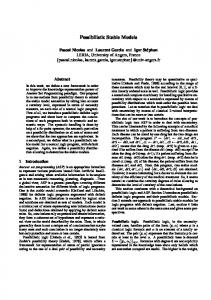
Fig. 7. MRE results. Mann-Whitey (95% confidence). These plots show number of losses of methods (a, b, c, d, e, f, g, h, i) against 158 methods as judged by Mann-Whitney (95% confidence). Each vertical set of marks shows results from 7 subsets of COC81 or 12 subsets of N ASA93.

COC81 MER Losses 150

150

100

100

50

50

0

0 a b c d e f g h i

Fig. 8.

NASA93 MER Losses

a b c d e f g h i

MER results. Mann-Whitey (95% confidence). Same rig as Figure 7.

E. Methods Not Explored We make no claim that this study explores the entire space of possible effort estimation methods: • Many more methods are listed in [50] (Figure 1) and in the first figure of this paper; • The reader may know of other effort estimation methods they believe we should try. Alternatively, the reader may have a design or an implementation of a new kind of effort estimator. Therefore, it is appropriate to ask why we selected these 158 methods and not thousands of others. The answer has two parts, one that is pragmatic and another that is methodological. • Pragmatically, we explore these 158 methods since we have advocated them in prior publications. We are hence required to determine if some (many) of them are sub-standard. • Methodologically, before it can be shown that an existing or new method is better than those we advocate here, we first need a demonstration that it is possible to make stable conclusions regarding the relative merits of different estimation methods. This paper offers such a demonstration.

SUBMITTED TO ASE JOURNAL, NOVEMBER 2009

13

COC81 AR Losses 150

150

100

100

50

50

0

Results using random seed1 :

0 a b c d e f g h i

a b c d e f g h i

COC81 AR Losses

NASA93 AR Losses

150

150

100

100

50

50

0

Results using random seed2 :

0 a b c d e f g h i

a b c d e f g h i

COC81 AR Losses

NASA93 AR Losses

150

150

100

100

50

50

0

Results using random seed3 : Fig. 9.

NASA93 AR Losses

0 a b c d e f g h i

a b c d e f g h i

AR results, repeated three different times with three different random seeds. Same rig as Figure 7.

VI. R ESULTS Figures 7, 8, and 9 show results from 20 repeats of: • Dividing some subset into T rain and T est sets. Note that in the special case of method e, the “subset” was all the data from one source. • Learning an effort model from the T rain set using COSEEKMO’s 158 methods; • Applying that model to the T est set; • Collecting performance statistics from the T est set using AR, MER, or MRE; • Reporting the number of times a method loses, where “loss” is determined by a Mann-Whitney U

SUBMITTED TO ASE JOURNAL, NOVEMBER 2009

14

test (95% confidence); Each mark on these plots shows the number of times a method loses in seven COC81 subsets (left plots) and twelve N ASA93 subsets (right plots). The x-axis shows results from the methods (a, b, c, d, e, f, g, h, i) described in Figure 6. In these plots, methods that generate lower losses are better. For example, the top-left plot of Figure 9 shows results for ranking methods applied to COC81 using AR. In that plot, all of the methods (a, d) result from the seven COC81 subsets that can be seen as y = losses ≈ 0. That is, in that plot, these two methods never lose against the other 158 methods. In these results, conclusion instability due to changing evaluation criteria can be detected by comparing results across Figures 7, 8, and 9. Also, conclusion instability due to changing subsets can be detected by comparing results across different subsets; either across the two sources, COC81 and N ASA9, or across their subsets selected during cross validation. In order to make this test more thorough, we also conducted the study using different random seeds controlling T rain and T est set generation (i.e. the three runs of Figure 9 that used different random seeds). A single glance shows our main result: the plots are very similar. Specifically, the (a, b, c, d) results fall very close to y = 0 losses. The significance of this result is discussed below. There are some instabilities in our results. For example, the exemplary performance of methods (a, d) in the top-left plot of Figure 9 does not repeat in other plots. For example, in the N ASA93 MRE and MER results shown in Figure 7 and Figure 8, method b loses much less than methods (a, d). However, in terms of number of losses generated by methods (a, b, c, d, e, f, g, h, i), the following two results holds across all evaluation criteria and all subsets and all seeds: 1) One member of method (a, b, c, d) always performs better (loses least) than all members of methods (e, f, g, h). Also, all members of methods (e, f, g, h) perform better than i. 2) Compared to 158 methods, one member of (a, b, c, d) always loses at some rate very close to zero. In our results, there is no single universal “best” method. Nevertheless, out of 158 methods, there are 154 clearly inferior methods. Hence, we recommend ranking methods (a, b, c, d) on all the available historical data, then applying the best ranked method to estimate new projects. VII. D ISCUSSION With the exception of the final notes on NEAREST, the following discussion notes should not be generalized beyond COCOMO-style data sets. The methods recommended above are strong endorsements of Boehm’s 1981 estimation research. All our “best” methods are based around Boehm’s preferred method for calibrating generic COCOMO models to local data. Method a is Boehm’s local calibration (or LC) procedure (defined in the appendix). This result endorses three of Boehm’s 1981 assumptions about effort estimation: Boehm’81 assumption 1: Effort can be modeled as a single function that is exponential on lines of code . . . Boehm’81 assumption 2: . . . and linearly proportional to the product of a set of effort multipliers; Boehm’81 assumption 3: The effort multipliers influence the effort by a set of pre-defined constants that can be taken from Boehm’s textbook [1]. Our results argue that there is little added value in methods (e, f, g, h, i), at least for our COCOMOstyle data sets. This is a useful result since these methods contain some of our slowest algorithms. For example, the WRAPPER column selection method used in (f, g, h) is an elaborate heuristic search through, potentially, many combinations. The failure of model trees in method f is also interesting. If the model trees of method f had outperformed (a, b, c, d), that would have suggested that effort is a multi-parametric phenomenon where, e.g.

SUBMITTED TO ASE JOURNAL, NOVEMBER 2009

15

over some critical size of software, different effects emerge. This proved not to be the case, endorsing Boehm’s assumption that effort can be modeled as a single parametric log-linear equation. Note that method e often performs better than other methods. This is partial evidence that increasing the training set size can be as useful as trying smarter algorithms. However, note that method e was always beaten by one of (a, b, c, d). Clearly, the value of training sets specialized to particular subsets can be enhanced by row and column pruning. Of all the methods in Figure 6, (a, b, c, d) perform the best and i performed the worst. The methods (a, b, c, d) lost less than 20 times in all runs while the NEAREST method used in i lost thousands of times. Why? One distinguishing feature of method i is the assumptions it makes about the domain. The NEAREST neighbor method i is assumption-less since it makes none of the Boehm’81 assumptions listed above. We hypothesize that Boehm’s assumptions are useful when processing COCOMO data. To the above comment, we hasten to add that while NEAREST performed relatively worse in isolation, we still believe that nearest neighbor methods like NEAREST are a valuable addition to any effort estimation toolkit: • Nearest neighbors used in conjunction with other methods can be quite powerful. For example, in the above resultss: – Two of the four methods that were consistently better than the rest were {c, d}; – Both these methods used LOCOMO to find nearest neighbors. • As mentioned above, not all domains are described in terms that can be used by the parametric forms like COCOMO. If the available domain data is in another format favorable to some of the other learners, then it is possible that our ranking orders would change. For example, Shepperd & Schofield argue that their case-based reasoning methods, like NEAREST procedure used in method i, are better suited to sparse data domains where precise numeric values are not available on all factors [39]. None of the data used in the study were sparse. VIII. E XTERNAL VALIDITY This study has several biases, listed below. Biases in the paradigm: This paper explores model-based methods (e.g. COCOMO ) and not expertbased methods. Model-based methods use some algorithm to summarize old data and make predictions about new projects. Expert-based methods use human expertise (possibly augmented with process guidelines or checklists) to generate predictions. Jorgensen [4] argues that most industrial effort estimation is expert-based and lists 12 best practices for such effort-based estimation. The comparative evaluation of model-based vs. expert-based methods must be left for future work. The evaluation of expert-based methods will be a human-intensive study and human subjects may rebel at participating in the lengthy experimental procedure described below. Before comparing any effort estimation methods (be they modelbased or expert-based), we must prune the space of model-based methods. For more on expert-based methods, see [4], [35], [39], [51]. Evaluation bias: We showed conclusion stability across three criteria; absolute residual; magnitude of error relative to estimate; or magnitude of relative error. This does not mean that we have shown stability across all possible evaluation biases. Other evaluation biases may offer different rankings to our estimation methods. Sampling bias: Model-based estimation methods use data and so are only useful in organizations that maintain historical data. Such data collection is rare in organizations with low process maturity. However, it is common elsewhere; e.g. amongst government contractors whose contract descriptions include process auditing requirements. For example, United States government contracts often require a model-based estimate at each project milestone. Such models are used to generate estimates or to double-check an expert-based estimate.

SUBMITTED TO ASE JOURNAL, NOVEMBER 2009

16

Another source of sampling bias is that the data sets used in this study come from two sources: (1) Boehm’s 1981 text on Software Engineering [1] and (2) data collected from NASA in the 1980s and 1990s from six different NASA centers, including the Jet Propulsion Laboratory (for details on this data, see the appendix). When we show our results to researchers in the field, they ask if two sources is enough to draw valid external conclusions. In reply, we comment that these two sources were repositories that accepted data from a wide range of projects. For example, our NASA data comes from different teams working at geographical locations spread throughout the United States using a variety of programming languages. While some of our data is from flight systems (a particular NASA specialty), most are ground systems and share many of the properties of other terrestrial software (same operating systems, development languages, development practices). Much of NASA’s software is written by contractors who service a wide range of clients (not just NASA). These contractors are contractually obliged (ISO-9001) to demonstrate their understanding and usage of current industrial best practices. For this reason, prior research has argued that conclusions from NASA data are relevant to the general software engineering industry. Basili, Zelkowitz, et al. [52], for example, published extensively for decades their conclusions taken from NASA data. Yet another source of sampling bias is that our conclusions are based only on the data sets studied here. The data used in this study is the largest public domain set of COCOMO-style data available. Also, our data source is as large as the proprietary COCOMO data sets used in prior TSE publications [35]. Biases in the model: This study adopts the COCOMO model for all its work. This decision was forced on us: the COCOMO-style data sets, described in the appendix, are the only public domain data we could access. Also, all our previous work was based on COCOMO data since our funding body (NASA) makes extensive use of COCOMO. The implications of our work on other estimation frameworks is an open and (as mentioned in the introduction) pressing issue. We strongly urge researchers with access to non-COCOMO data to repeat the kind of row/column pruning analysis described here. IX. C ONCLUSION This paper concludes five years of research that began with the following question; can the new generation of data miners offer better effort estimates than traditional methods? In other work [11], we detected no improvement using bagging [53] and boosting [54] methods for COCOMO-style data sets. In this work, we have found that one of four methods is always better than another 154 methods: • A single linear model is adequate for the purposes of effort estimation. All the methods that assume multiple linear models, such as model trees (f ), or no parametric form at all, such as nearest neighbor (i), perform relatively poorly. F • Elaborate searches do not add value to effort estimation. All the O(2 ) column pruners do worse than near-linear-time column pruning. • The more intricate methods such as model trees do no better than other methods. Unlike Shepperd & Kadoda’s results, we were able to find stable conclusions across different data sets, different random number seeds, and even different evaluation criteria. Consequently, we argue for both a complication and simplification of effort estimation research: • Complication #1: One reason for not using COCOMO is that the available data has to be expressed in terms of the COCOMO features, which is problematic if companies have not collected their historical data using the COCOMO ontology. Nevertheless, our results suggest that it may be worth the effort to use COCOMO-style data collection, if only to reduce the instability in the conclusions. • Complication #2: Simply applying one or two methods in a new domain is not enough. In the study reported in this paper, one method out of a set of four was always the best but that best method was data set-specific. Therefore, prior to researchers drawing conclusions about aspects of effort estimation properties in a particular context, there should be a selection study to rank and prune the available estimators according to the details of a local domain.

SUBMITTED TO ASE JOURNAL, NOVEMBER 2009

17

Simplification: Fortunately, our results also suggest that such selection studies need not be very = 97% of the methods implemented elaborate. At least for COCOMO-style data, we report that 154 158 in our COSEEKMO toolkit [26] added little or nothing to Boehm’s 1981 regression procedure [1]. Such a selection study could proceed as follows. For COCOMO-style data sets, the following methods should be tried and the one that does best on historic data (assessed using Mann-Whitney U test) should be used to predict new projects: • Adopt the three Boehm’81 assumptions and use LC-based methods. F • While some row and column pruning can be useful, elaborate column pruning (requiring an O(2 ) search) is not. Hence, try LC with zero or more of LOCOMO’s row pruning or COCOMIN’s column pruning. For future work, we recommend an investigation of a certain ambiguity in our results: • Prior experiments found conclusion instability after limited application of row and column pruning to non-COCOMO features. • Here, we found conclusion stability after extensive row and column pruning to COCOMO-style features. It is hence unclear what removed the conclusion instability. Was it pruning? Or the use of the COCOMO features? To test this, we require a new kind of data set. Given examples expressed in whatever local features are available, those examples should be augmented with COCOMO features. Then, this study should be repeated: • With and without the local features; • With and without the COCOMO features; • With and without pruning; We would be interested in contacting any industrial group with access to this new kind of data set. •

ACKNOWLEDGMENTS Martin Shepperd was kind enough to make suggestions about different evaluation biases and the design of the NEAREST and LOCOMO methods. A PPENDIX A. Data Used in This Study In this study, effort estimators were built using all or some part of data from two sources: COC81: 63 records in the COCOMO-I format. Source: [1, p496-497]. Download from http:// unbox.org/wisp/trunk/cocomo/data/coc81modeTypeLangType.csv. N ASA93: 93 NASA records in the COCOMO-I format. Download from http://unbox.org/ wisp/trunk/cocomo/data/nasa93.csv. Taken together, these two sets are the largest COCOMO-style data source in the public domain (for reasons of corporate confidentiality, access to Boehm’s COCOMO-II data set is highly restricted). N ASA93 was originally collected to create a NASA-tuned version of COCOMO, funded by the Space Station Freedom Program and contains data from six NASA centers, including the Jet Propulsion Laboratory. For more details on this data set, see [26]. Different subsets and number of subsets used (in parenthesis) are: All(2): selects all records from a particular source. Category(2):N ASA93 designation selecting the type of project; e.g. avionics. Center(2): N ASA93 designation selecting records relating to where the software was built. Fg(1): N ASA93 designation selecting either “f ” (flight) or “g” (ground) software. Kind(2):COC81 designation selecting records relating to the development platform; e.g. max is mainframe.

SUBMITTED TO ASE JOURNAL, NOVEMBER 2009

18

Lang(2): COC81 designation selecting records about different development languages; e.g ftn is FORTRAN. Mode(4): designation selecting records relating to the COCOMO-I development mode: one of semidetached, embedded, and organic. Project(2): N ASA93 designation selecting records relating to the name of the project. Year(2): is a N ASA93 term that selects the development years, grouped into units of five; e.g. 1970, 1971, 1972, 1973, 1974 are labeled “1970”. There are more than 19 data sets overall. Some have fewer than 20 projects and hence were not used. The justification for using 20 projects or more is offered in [26]. B. Learners Used in This Study 1) Learning with Model Trees: Model trees are a generalization of linear regression. Instead of fitting the data to one linear model, model trees learn multiple linear models, and a decision tree that decides which linear model to use. Model trees are useful when the projects form regions and different models are appropriate for different regions. COSEEKMO includes the M5p model tree learner defined by Quinlan [48]. 2) Other Learning Methods: See the Related work section for notes on learning with linear regression; local calibration; and nearest neighbor methods. C. Pre-Processors Used in This Study 1) Pre-processing with Row Pruning: The LOCOMO tool [45] in COSEEKMO is a row pruner that combines a nearest neighbor method with LC. LOCOMO prunes away all projects except those k “nearest” to the T est set data. To learn an appropriate value for k, LOCOMO uses the T rain set as follows: • For each project p0 ∈ T rain, LOCOMO sorts the remaining T rain − p0 examples by their Euclidean distance from p0 . • LOCOMO then passes the k0 examples closest to p0 to LC. The returned < a, b > values are used to estimate effort for p0 . • After trying all possible k0 values, 2 ≤ k0 ≤ |T rain|, k is then set to the k0 value that yielded the smallest mean MRE7 . This calculated value k is used to estimate the effort for projects in the T est set. For all p1 ∈ T est, the k nearest neighbors from T rain are passed to LC. The returned < a, b > values are then used to estimate the effort for p1 . 2) Pre-Processing with Column Pruning: Kirsopp & Schofeld [41] and Chen & Menzies & Port & Boehm [42] report that column pruning improves effort estimation. Miller’s research [40] explains why. Column pruning (a.k.a. feature subset selection [17] or variable subset selection [40]) reduces the deviation of a linear model learned by minimizing least squares error [40]. To see this, consider a linear model with constants βi that inputs features fi to predict for y: y = β0 + β1 · f1 + β2 · f2 + β3 · f3 ... The variance of y is some function of the variances in f1 , f2 , etc. If the set F contains noise, then random variations in fi can increase the uncertainty of y. Column pruning methods decrease the number of features fi , thus increasing the stability of the y predictions. That is, the fewer the features (columns), the more restrained are the model predictions. Taken to an extreme, column pruning can reduce y’s variance to zero (e.g. by pruning the above equation back to y = β0 ) but increases model error (the equation y = β0 will ignore all project data when 7

A justifications for using the mean measure within LOCOMO is offered at the end of the appendix.

SUBMITTED TO ASE JOURNAL, NOVEMBER 2009

19

generating estimates). Hence, intelligent column pruners experiment with some proposed subsets F 0 ⊆ F before changing that set. COSEEKMO currently contains three intelligent column pruners: WRAPPER, LOCALW, and COCOMIN. WRAPPER [47] is a standard best-first search through the space of possible features. At worst, WRAPPER must search a space exponential on the number of features F ; i.e. 2F . However, a simple best-first heuristic makes WRAPPER practical for effort estimation. At each step of the search, all the current subsets are scored by passing them to a target learner. If a set of features does not score better than a smaller subset, then it gets one “mark” against it. If a set has more than ST ALE = 5 number of marks, it is deleted. Otherwise, a feature is added to each current set and the algorithm continues. In general, a WRAPPER can use any target learner. Chen’s LOCALW is a WRAPPER specialized for LC. Previously [26], [42], we have explored LOCALW for effort estimation. The above description of WRAPPER should be read as a brief introduction to all the techniques associated with this kind of column pruner. A WRAPPER is a powerful tool and can be extensively and usefully customized (e.g. using a hash-table cache to hold the frequently seen combinations; alternative search methods to best-first search; etc). We refer the interested reader to the thorough treatment of the subject found in Miller [40] and Kohavi & Johns [47]. Theoretically, WRAPPER (and LOCALW)’s exponential time search is more thorough, hence more useful, than simpler methods that try fewer options. To test that theory, we will compare WRAPPER and LOCALW to a linear-time column pruner called COCOMIN [11]. COCOMIN is defined by the following operators: {sorter, order, learner, scorer} The algorithm runs in linear time over a sorted set of features, F . This search can be ordered in one of two ways: • A “backward elimination” process starts with all features F and throws some away, one at a time. • A “forward selection” process starts with one feature and adds in the rest, one at a time. Regardless of the search order, at some point the current set of features F 0 ⊆ F is passed to a learner to generate a performance score by applying the model learned on the current features to the T rain set. COCOMIN returns the features associated with the highest score. COCOMIN pre-sorts the features on some heuristic criteria. Some of these criteria, such as standard deviation or entropy, are gathered without evaluation of the target learner. Others are gathered by evaluating the performance of the learner using only the feature in question plus any required features, such as KLOC for COCOMO, to calibrate the model. After the features are ordered, each feature is considered for backward elimination, or forward selection if chosen, in a single linear pass through the feature space, F . The decision to keep or discard the feature is based on an evaluation measure generated by calibrating and evaluating the model with the training data. Based on [11], the version of COCOMIN used in this study: • sorted the features by the highest median MRE; • used a backward elimination search strategy; • learned using LC; • scored using mean MRE. Note that mean MRE is used internally to COCOMIN (and LOCOMO, see above) since it is fast and simple to compute. Once the search terminates, this paper strongly recommends the more thorough (and hence more intricate and slower) median non-parametric measures to assess the learned effort estimation model.

SUBMITTED TO ASE JOURNAL, NOVEMBER 2009

20

R EFERENCES [1] B. Boehm, Software Engineering Economics. Prentice Hall, 1981. [2] C. Kemerer, “An empirical validation of software cost estimation models,” Communications of the ACM, vol. 30, no. 5, pp. 416–429, May 1987. [3] Spareref.com, “Nasa to shut down checkout & launch control system,” August 26, 2002, http://www.spaceref.com/news/viewnews.html? id=475. [4] M. Jorgensen, “A review of studies on expert estimation of software development effort,” Journal of Systems and Software, vol. 70, no. 1-2, pp. 37–60, 2004. [5] M. Jorgensen and M. Shepperd, “A systematic review of software development cost estimation studies,” January 2007, available from http://www.simula.no/departments/engineering/publications/Jorgensen.200%5.12. [6] L. Briand, T. Langley, and I. Wieczorek, “A replicated assessment and comparison of common software cost modeling techniques,” in Proceedings of the 22nd International Conference on Software Engineering, Limerick, Ireland, 2000, pp. 377–386. [7] K. Lum, J. Powell, and J. Hihn, “Validation of spacecraft software cost estimation models for flight and ground systems,” in ISPA Conference Proceedings, Software Modeling Track, May 2002. [8] D. Ferens and D. Christensen, “Calibrating software cost models to Department of Defense Database: A review of ten studies,” Journal of Parametrics, vol. 18, no. 1, pp. 55–74, November 1998. [9] I. H. Witten and E. Frank, Data mining. 2nd edition. Los Altos, US: Morgan Kaufmann, 2005. [10] E. Mendes, I. D. Watson, C. Triggs, N. Mosley, and S. Counsell, “A comparative study of cost estimation models for web hypermedia applications,” Empirical Software Engineering, vol. 8, no. 2, pp. 163–196, 2003. [11] D. Baker, “A hybrid approach to expert and model-based effort estimation,” Master’s thesis, Lane Department of Computer Science and Electrical Engineering, West Virginia University, 2007, available from https://eidr.wvu.edu/etd/documentdata.eTD?documentid=5443. [12] T. Menzies, Z. Chen, J. Hihn, and K. Lum, “Selecting Best Practices for Effort Estimation,” IEEE Transactions on Software Engineering, vol. 32, pp. 883–895, 2006. [13] Y. Li, M. Xie, and G. T., “A study of the non-linear adjustment for analogy based software cost estimation,” Empirical Software Engineering, pp. 603–643, 2009. [14] J. W. Keung, B. A. Kitchenham, and D. R. Jeffery, “Analogy-x: Providing statistical inference to analogy-based software cost estimation,” IEEE Trans. Softw. Eng., vol. 34, no. 4, pp. 471–484, 2008. [15] C. Chang, “Finding prototypes for nearest neighbor classifiers,” IEEE Trans. on Computers, pp. 1179–1185, 1974. [16] Y. Li, M. Xie, and T. Goh, “A study of project selection and feature weighting for analogy based software cost estimation,” Journal of Systems and Software, vol. 82, pp. 241–252, 2009. [17] M. Hall and G. Holmes, “Benchmarking attribute selection techniques for discrete class data mining,” IEEE Transactions On Knowledge And Data Engineering, vol. 15, no. 6, pp. 1437– 1447, 2003, available from http://www.cs.waikato.ac.nz/∼mhall/HallHolmesTKDE.pdf. [18] J. Gama and C. Pinto, “Discretization from data streams: applications to histograms and data mining,” in SAC ’06: Proceedings of the 2006 ACM symposium on Applied computing. New York, NY, USA: ACM Press, 2006, pp. 662–667, available from http: //www.liacc.up.pt/∼jgama/IWKDDS/Papers/p6.pdf. [19] U. M. Fayyad and I. H. Irani, “Multi-interval discretization of continuous-valued attributes for classification learning,” in Proceedings of the Thirteenth International Joint Conference on Artificial Intelligence, 1993, pp. 1022–1027. [20] Y. Yang and G. I. Webb, “A comparative study of discretization methods for naive-bayes classifiers,” in Proceedings of PKAW 2002: The 2002 Pacific Rim Knowledge Acquisition Workshop, 2002, pp. 159–173. [21] U. Lipowezky, “Selection of the optimal prototype subset for 1-NN classification,” Pattern Recognition Letters, vol. 19, p. 907918, 1998. [Online]. Available: http://linkinghub.elsevier.com/retrieve/pii/S0167865598000750 [22] F. Walkerden and R. Jeffery, “An empirical study of analogy-based software effort estimation,” Empirical Softw. Engg., vol. 4, no. 2, pp. 135–158, 1999. [23] C. Kirsopp and M. Shepperd, “Making inferences with small numbers of training sets,” IEEE Proc., vol. 149, 2002. [24] M. Shepperd and G. F. Kadoda, “Comparing software prediction techniques using simulation,” IEEE Trans. Software Eng, vol. 27, no. 11, pp. 1014–1022, 2001. [25] B. Boehm, “A spiral model of software development and enhancement,” Software Engineering Notes, vol. 11, no. 4, p. 22, 1986. [26] T. Menzies, Z. Chen, J. Hihn, and K. Lum, “Selecting best practices for effort estimation,” IEEE Transactions on Software Engineering, November 2006, available from http://menzies.us/pdf/06coseekmo.pdf. [27] R. Park, “The central equations of the price software cost model,” in 4th COCOMO Users Group Meeting, November 1988. [28] R. Jensen, “An improved macrolevel software development resource estimation model,” in 5th ISPA Conference, April 1983, pp. 88–92. [29] L. Putnam and W. Myers, Measures for Excellence. Yourdon Press Computing Series, 1992. [30] R. A. Endres, H.D, “A handbook of software and systems engineering: Empirical observations, laws and theories,” 2003. [31] S. Gregor, “Design theory in information systems,” Australasian Journal of Information Systems, December 2002, available from http://dl.acs.org.au/index.php/ajis/article/viewPDFInterstitial/439/399%?ads=. [32] J. Anderson, Cognitive Psychology and its Implications. W.H. Freeman and Company, 1985. [33] D. Simons and C. Chabris, “Gorillas in our midst: Sustained inattentional blindless for dynamic events perception,” Perception, vol. 28, pp. 1059–1074, 1999. [34] M. Shepperd, “Software project economics: A roadmap,” in International Conference on Software Engineering 2007: Future of Software Engineering, 2007. [35] S. Chulani, B. Boehm, and B. Steece, “Bayesian analysis of empirical software engineering cost models,” IEEE Transaction on Software Engineerining, vol. 25, no. 4, July/August 1999. [36] B. Boehm, E. Horowitz, R. Madachy, D. Reifer, B. K. Clark, B. Steece, A. W. Brown, S. Chulani, and C. Abts, Software Cost Estimation with Cocomo II. Prentice Hall, 2000.

SUBMITTED TO ASE JOURNAL, NOVEMBER 2009

21

[37] J. Li and G. Ruhe, “Decision support analysis for software effort estimation by analogy,” in Proceedings, PROMISE’07 workshop on Repeatable Experiments in Software Engineering, 2007. [38] B. A. Kitchenham, E. Mendes, and G. H. Travassos, “Cross- vs. within-company cost estimation studies: A systematic review,” IEEE Transactions on Software Engineering, pp. 316–329, May 2007. [39] M. Shepperd and C. Schofield, “Estimating software project effort using analogies,” IEEE Transactions on Software Engineering, vol. 23, no. 12, November 1997, available from http://www.utdallas.edu/∼rbanker/SE XII.pdf. [40] A. Miller, Subset Selection in Regression (second edition). Chapman & Hall, 2002. [41] C. Kirsopp and M. Shepperd, “Case and feature subset selection in case-based software project effort prediction,” in Proc. of 22nd SGAI International Conference on Knowledge-Based Systems and Applied Artificial Intelligence, Cambridge, UK, 2002. [42] Z. Chen, T. Menzies, D. Port, and B. Boehm, “Finding the right data for software cost modeling,” IEEE Software, Nov 2005. [43] J. Kliijnen, “Sensitivity analysis and related analyses: a survey of statistical techniques,” Journal Statistical Computation and Simulation, vol. 57, no. 1–4, pp. 111–142, 19987. [44] T. Menzies, D. Port, Z. Chen, J. Hihn, and S. Stukes, “Validation methods for calibrating software effort models,” in Proceedings, ICSE, 2005, available from http://menzies.us/pdf/04coconut.pdf. [45] O. Jalali, “Evaluation bias in effort estimation,” Master’s thesis, Lane Department of Computer Science and Electrical Engineering, West Virginia University, 2007. [46] H. B. Mann and D. R. Whitney, “On a test of whether one of two random variables is stochastically larger than the other,” Ann. Math. Statist., vol. 18, no. 1, pp. 50–60, 1947, available on-line at http://projecteuclid.org/DPubS?service=UI&version=1.0&verb= Display&hand%le=euclid.aoms/1177730491. [47] R. Kohavi and G. H. John, “Wrappers for feature subset selection,” Artificial Intelligence, vol. 97, no. 1-2, pp. 273–324, 1997. [Online]. Available: citeseer.nj.nec.com/kohavi96wrappers.html [48] J. R. Quinlan, “Learning with Continuous Classes,” in 5th Australian Joint Conference on Artificial Intelligence, 1992, pp. 343–348, available from http://citeseer.nj.nec.com/quinlan92learning.html. [49] T. Menzies, Z. Chen, D. Port, and J. Hihn, “Simple software cost estimation: Safe or unsafe?” in Proceedings, PROMISE workshop, ICSE 2005, 2005, available from http://menzies.us/pdf/05safewhen.pdf. [50] I. Myrtveit, E. Stensrud, and M. Shepperd, “Reliability and validity in comparative studies of software prediction models,” IEEE Transactions on Software Engineerining, vol. 31, no. 5, pp. 380–391, May 2005. [51] M. Jorgensen and K. Molokken-Ostvold, “Reasons for software effort estimation error: Impact of respondent error, information collection approach, and data analysis method,” IEEE Transactions on Software Engineering, vol. 30, no. 12, December 2004. [52] V. Basili, F. McGarry, R. Pajerski, and M. Zelkowitz, “Lessons learned from 25 years of process improvement: The rise and fall of the NASA software engineering laboratory,” in Proceedings of the 24th International Conference on Software Engineering (ICSE) 2002, Orlando, Florida, 2002, available from http://www.cs.umd.edu/projects/SoftEng/ESEG/papers/83.88.pdf. [53] L. Brieman, “Bagging predictors,” Machine Learning, vol. 24, no. 2, pp. 123–140, 1996. [54] Y. Freund and R. Schapire, “A decision-theoretic generalization of on-line learning and an application to boosting,” JCSS: Journal of Computer and System Sciences, vol. 55, 1997.