Apr 8, 1999 - A procedure is derived for computing standard errors in random intercept ..... Both quadrature formulae provide unbiased estimates and for ...
Standard Errors for EM Estimates in Variance Component Models Herwig Friedl�
Goran Kauermann y
April 8, 1999 Abstract A procedure is derived for computing standard errors in random intercept models for estimates obtained from the EM algorithm. We discuss two different approaches: a Gau�-Hermite quadrature for Gaussian random e�ect models and a nonparametric maximum likelihood estimation for an unspeci ed random e�ect distribution. An approximation of the expected Fisher information matrix is proposed which is based on an expansion of the EM estimating equation. This allows for inferential arguments based on EM estimates, as demonstrated by an example and simulations.
EM algorithm, Gau�-Hermite Quadrature, Nonparametric Maximum Likelihood, Estimating Equation. Keywords:
Institute of Statistics; Technical University Graz; Lessingstr. 27; 8010 Graz, Austria Institute of Statistics; Ludwig-Maximilians-University Munich; Akademiestr. 1; 80796 Munich, Germany �
y
1
1 Introduction We consider a generalized variance component model for n clusters of independent response variables yi = (yi ; : : : ; yin )t , i = 1; : : : ; n. The response yi is assumed to depend on the covariate matrix xi = (xi ; : : : ; xin )t and the unobservable random e�ect zi . The mean response is modeled by the conditional generalized linear model E (yij jzi; xij ) = �ij = h(xtij + zi) where h(�) is the inverse link function and 1
i
1
i
denotes the associated p dimensional parameter vector of interest. Conditional
on the random e�ect, the components of yi are assumed to be independent, i.e. Q f (yi jzi ; ) = j f (yij jzi ; ) where the density f (�j�) is assumed to be of exponential family form. For ni > 1 the model can be used for equi-correlated dependent observations, see e.g. Diggle et al. (1994, chapter 9) or Breslow & Clayton (1993) and references given there. If ni = 1 the model is known as random e�ect model which provides a general and convenient way for modeling overdispersion, see e.g. Aitkin (1996). The random e�ects zi, i = 1; : : : ; n, are assumed to be independently and identically distributed with density f (zi). Since the zi are unobserved this leads to the R observed (marginal) log likelihood l( ) = Pni log f (yijzi)f (zi)dzi which can be maximized by the iterative expectation maximization (EM) algorithm (see Dempster et al., 1977). In the t-th step this gives the function =1
n R X log ff (yijRzi ; )f (zi)g f (yijzi; t )f (zi)dzi ; Q( j ) = f (y jz ; t )f (z )dz ( )
(t)
i
i=1
i
( )
i
i
(1)
which has to be maximized in with t held xed. It is a traditional and also convenient approach to assume normally distributed random e�ects, which allows to approximate l( ) by a Gau�-Hermite (GH) quadrature. More exibility is however achieved by treating the e�ect distribution as unknown, as suggested by Aitkin ( )
2
(1996, 1999). This leads to nonparametric maximum likelihood (NPML) estimation as introduced by Laird (1978). In both settings the EM algorithm can be applied. A criticism of the EM algorithm is, that it does not automatically provide estimates for the variance-covariance matrix of the EM estimate ^. As pointed out in McLachlan & Krishnan (1997) for a variety of examples, this point is closely related to the problem of slow convergence. If the maximization of (1) is done by a NewtonRaphson procedure based on @ Q( j t )=@ @ t , directly applying successive E and M steps will provide an estimate of the complete information at convergence. How2
( )
ever, this does not account for the missing information on the unobservable random e�ects. Louis (1982) provides a very general derivation of the observed information matrix and shows that this matrix can be rewritten as a di�erence of the complete and the missing information. Oakes (1999) discusses a formula for the observed information which depend only on derivatives of Q(�). We suggest a simpli ed version of this approach yielding the appropriate measure of information { the estimated a priori expected information { which takes the special structure of the considered models into account, see also Meilijson (1989). In Section 2 we embed the EM algorithm in the framework of estimating equations. For both settings, GH approximation and NPML estimation, we expand the EM estimating equations. The rst order derivative provides an approximative variance for the estimates. In Section 3 we apply this variance approximation in a data example and investigate its small sample behavior by a simulation study.
3
2 EM Estimating Equations 2.1 Gaussian E�ects Assuming zi iid � N (0; 1), we can model �ij = h(xtij + zi�z ) which allows to approximate the integrals in l( ) by a quadrature formula like GH. Hinde (1982) uses this technique in random e�ect models, Anderson & Aitkin (1985) apply it to variance component models. The quadrature yields the approximation f (yi; �)
=
Z
f (yijzi ; �)'(zi )dzi �
K X k =1
f (yij�k ; �)�k
=: fK (yi; �);
(2)
where ' denotes the standard normal density function, � = ( t; �z )t and K is the number of approximation points. Note that for given K , the masspoints �k and their associated masses �k are known and available from tables. Applying this quadrature also to the nominator in (1), approximates Q(�) by QK (�j�
(t)
)=
n X K X i=1 k =1
(t) wik flog f (yij�k ; �) + log �k g
(3)
with weights wikt = f (yij�k ; � t )�k =fK (yi; � t ). These weights can thereby be seen as masses for the masspoints �k corresponding to the posterior distribution f (zijyi). Formula (3) represents the E-step of the underlying EM algorithm. The M-step is given by the p + 1 dimensional estimating equation ( )
( )
@QK (�j�(t) ) @�
( )
=
n X K X i=1 k =1
(t) wik sik
= 0:
(4)
with sik = sik (�) = @ log f (yij�k ; �)=@� denoting the i-th score contribution, given zi = �k . We embed the EM algorithm into the concept of estimating equations by de ning g� (�) =
@QK (�~j�) @ �~ �~=�
4
as estimating function for � (see also Oakes, 1999). It is easily seen that the EM estimate �^ solves g� (�^) = 0. Let now � denote the vector of true parameter values in the approximating density (2). This means EK fg� (�)g = 0, where subscript K indicates, that the expectation is calculated using the density fK (�). As in the usual likelihood theory, we can expand g� (�^) about � and nd in rst order approximation �^ ? � = ?
@g� (�) @�t
!?
1
g� (�):
Di�erentiation of g� (�) has to take into account that the weights !ik in (3) depend on �. Assuming f (yjz; �) to be of exponential family form one gets @!ik =@� = P !ik (sik ? l !il sil ). This yields @g� (�) @�t
=
n X K X i=1 k =1
�
wik sik stik +
n X K X K @sik � X ? wik wil sik stil : @�t i=1 k =1 l=1
(5)
Using density fK (�) we nd EK (wik sik stik ) = ?EK (wik @sik =@�t ) so that the rst component in (5) has zero expectation. Hence, we can approximate (5) in the usual likelihood fashion by the Fisher type matrix FK (�) := EK
? @g@�� (t�)
!
=
n X K X K X i=1 k =1 l=1
�
EK wik wil sik stil
�
�
�
= EK g� (�)g�t (�) : (6)
In rst order approximation one has varK (�^) = FK? (�) where the variance of the regression coe�cient ^ is obtained by extracting the corresponding submatrix of FK? (�). One should note that this implicitly takes the variability due to the estimation of the random e�ect variance �z into account. 1
1
2
Formula (5) can be related to the results given in Louis (1982). We can rewrite the observed information (5) as the di�erence of the complete and the missing information, again using the approximate density fK (�). Direct calculation provides the complete information Pni PKk wik @sik =@�t , whereas the remaining components in (5) give the missing information. Important for this assignment is the =1
=1
5
property that the random e�ect distribution does not depend on �. Therefore, the conditional scores sik can be also de ned as the complete scores evaluated at zi
= �k . Hence, si(�) := Pk wik sik gives an approximation of the i-th observed
score component, which is the conditional expectation of the corresponding complete score, given the data. Rewriting (6) as the sum of observed score variances,
i.e. FK (�) = Pni varK fsi(�)g, leads to the idea suggetsed in Meilijson (1989). He uses the empirical Fisher information matrix to estimate the Fisher information for identically distributed variates. The arguments above do not hold, if the e�ect den=1
sity is totally unknown. We show however that the estimating equation approach directly provides variance estimation also in this setting.
2.2 Unknown E�ect Distribution Let now f (z) be unknown so that and f (z) have to be estimated simultaneously by the NPML approach as suggested by Aitkin & Francis (1995) or Aitkin (1996, 1999), see also Laird (1978). This approach directly generalizes (3), however now � = (� ; : : : ; �K )t and � = (� ; : : : ; �K )t are both treated as unknown and are estimated from the data. Like in the previous section, Q(�j�) is used to approximate (1) with � = ( t ; � t)t and � as unknown parameters. We get (4) as M-step for � and the masses are obtained from �kt = Pni niwikt = Pni ni . For the following expansion of the EM estimating equations it is helpful to reparameterize � by the canonical multinomial representation �k = expf#k ? �(#)g for k = 1; : : : ; K ? 1. This guarantees �k > 0 for all # = (# ; : : : ; #K ? )t 2 1) + ti t + ti�(j > 1) t g 1
(10)
1
where �(j > 1) is an indicator for the period, i.e. �(j > 1) = 1 for j > 1 and zero otherwise. In (10) t gives the therapy e�ect, adjusts for a placebo e�ect while 1
1
t copes for a possible randomization e�ect.
We t model (10) by NPML estimation which suggests K = 9 distinct masspoints. If a model with K > 9 masspoints is tted, the resulting additional masspoints either do not di�er from these 9 or have negligible masses. The resulting distribution function from �^ and �^ is plotted in Figure 1 and shows a uniform shape. Table 1 gives the estimates for the regression coe�cients with variances calculated by Monte Carlo integration. We also used a Gau� Hermite quadrature (K=12) to t the data where the corresponding tted random e�ect distribution is also shown in Figure 1. The GH estimates hardly di�er from the NPML estimates. Also the inference allows for similar interpretations. The estimated variances resemble those given in Diggle et al. which are based on a normal approximation of the likelihood as suggested by Breslow & Clayton (1993). (Table 1 and Figure 1 about here)
3.2 Simulation We run a simulation study to investigate the small sample behavior of the suggested variance approximation. We consider the model yij jzi � Poissonf�i = 1+ zi + xij g, i = 1; : : : ; n and j = 1; : : : ; ni with = 1, n = 40 and ni = 2. The covariate xij is taken as binary factor, i.e. xij 2 f0; 1g, with balanced design in the sense xi = xi 1
9
2
and xij = 1 for half of the data. The zi 's are drawn from the three settings: normal: zi � N 8 (0; 0:5 ); > < N (0; 0:3 ) with probability 0:5 b) mixed: zi � > : 8 N (1; 0:3 ) with probability 0:5; > < N (0; 0:3 ) with probability 0:9 c) contaminated: zi � > : N (1:5; 0:1 ) with probability 0:1: We t the model by NPML estimation starting with K = 8 masspoints and reducing K until all masspoints are di�erent. We also use a GH quadrature with K = a)
2
2
2
2
2
16 masspoints. Table 2 shows the mean and standard deviation of 2-0 simulated estimates. Both quadrature formulae provide unbiased estimates and for settings a) and b) they show the same variability. In setting c) however the NPML estimate is clearly less variable than a GH estimate. In general, NPML estimation shows to be not less e�cient than GH estimation, even if random e�ects are normally distributed where the GH procedure gives the right quadrature. Moreover the NPML approach can cope for non-normality of the random e�ect distribution. In Table 2 we also report the coverage probability of con dence intervals based on the suggested standard errors. The variance approximations show to work reasonably well with a slightly liberal character though. In the contaminated case on the other hand, the NPML con dence bands are conservative. In general, con dence bands based on NPML estimates behave rather promissing in all three settings. (Table 2 about here)
4 Results and Conclusions The above results suggest a variance approximation of EM estimates in random e�ect models based on quadrature formulae. Assuming the di�erences between the 10
density f (�) of the random e�ect and its approximation fK (�) to be negligible, we can use Fisher type matrices for variance estimation. The same arguments used above also allows to examine di�erences between masspoints �j and �k or the relevance of the masses �k . This indirectly gives an exploratory procedure to evaluate the number K of masspoints used and comply with the proposals in Laird (1978).
References Aitkin, M. (1996). A general maximum likelihood analysis of overdispersion in generalized linear models. Statistics and Computing, 6, 251-262. Aitkin, M. (1999). A general maximum likelihood analysis of variance components in generalized linear models. Biometrics, 55, 218-234. Aitkin, M., Francis, B.J. (1995). Fitting overdispersed generalized linear models by nonparametric maximum likelihood. The GLIM Newsletter, 25, 37-45. Anderson, D.A., Aitkin, M. (1985). Variance component models with binary response: interviewer variability. Journal of the Royal Statistical Society, Series B, 47, 203-210. Breslow, N.E., Clayton, D.G. (1993). Approximate inference in generalized linear mixed models. Journal of the American Statistical Association, 88, 9-25. Dempster, A.P., Laird, N.M., Rubin, D.B. (1977). Maximum likelihood estimation from incomplete data via the EM algorithm. (with discussion). Journal of the Royal Statistical Society B, 39, 1-38. Diggle, P.J., Liang, K.-Y., Zeger, S.L. (1994). Analysis of longitudinal data. Oxford University Press, Oxford 11
Hinde, J. (1982). Compound Poisson regression models. In: GLIM 82 (R. Gilchrist, ed.), 109-121. Springer-Verlag, New York. Laird, N. (1978). Nonparametric maximum likelihood estimation of a mixing distribution. Journal of the American Statistical Association, 73, 805-811. Louis, T.A. (1982). Finding the observed information matrix when using the EM algorithm. Journal of the Royal Statistical Society B, 44, 226-233. McLachlan, G.J., Krishnan, T. (1997). The EM Algorithm and Extensions. John Wiley & Sons, Inc., New York. Meilijson, I. (1989). A fast improvement to the EM algorithm on its own terms. Journal of the Royal Statistical Society B, 51, 127-138. Oakes, D. (1999). Direct calculation of the information matrix via the EM algorithm. Journal of the Royal Statistical Society, Series B, 61, 479-482. Thall, P.F., Vail, S.C. (1990). Some Covariance Models for Longitudinal Count Data With Overdispersion. Biometrics, 46, 537{547.
12
NPML GH
0.0
0.2
probability 0.4 0.6
0.8
1.0
Distribution of random effects
-0.5
0.0
0.5
1.0
1.5
z
Figure 1: Estimated random e�ect distribution for epileptic seizure data NPMLE Fit e�ect ^ pvar( ^) t -.126 .194 .121 .084 t -.295 -.079 1
1
Gau�-Hermite Fit pvar( ^) ^ .048 .070 .122 .052 -.298 .083
Table 1: Estimates and standard errors for epileptic seizure data random e�ect
mean( ^) s.e.( ^) NPMLE normal 0.98 .21 mixed 1.02 .22 contaminated 1.00 .07 GH normal .99 .22 mixed .98 .20 contaminated 1.00 .23
coverage 90 % 95 % 87.1 83.3 93.8
92.6 87.9 98.1
87.0 84.8 84.5
91.5 91.4 91.0
Table 2: Mean and standard error of EM estimates and the resulting coverage probability of con dence intervals based on 200 simulations. i