A Component-wise EM Algorithm for Mixtures

arXiv:1201.5913v1 [stat.CO] 27 Jan 2012

A Component-wise EM Algorithm for Mixtures

Abstract: Estimation finite mixture distributions is typically an incomplete data structure problem for which the Expectation-Maximization (EM) algorithm can be used. One drawback of the algorithm is its slow convergence in some situations. In the mixtures case, little progress in speeding up EM has been made. Standard EM procedures update all parameters simultaneously. In the missing data context, it has been shown that sequential updating could lead to faster convergence. In this paper we propose a component-wise EM for mixtures, which updates the parameters sequentially. It intrinsically decouples the parameter updates so that the estimated proportions may not sum to 1 during an iteration. While maintaining monotone convergence, the algorithm may leave the parameter space but is guaranteed to return upon convergence. We give an interpretation of this procedure as a proximal point algorithm and use it to prove the convergence. Illustrative numerical experiments show how our algorithm compares to EM and a version of the SAGE algorithm. [un mot sur les perf]

Key-words: EM algorithm, Kullback-Leibler divergence, Mixture estimation, Proximal point algorithm, SAGE algorithm.

1

1

Introduction

Estimation in finite mixture distributions is typically an incomplete data structure problem for which the EM algorithm is used (see for instance Dempster, Laird and Rubin 1977 and Redner and Walker 1984). The most documented problem occuring with the EM algorithm is its possible low speed in some situations. Many papers have proposed extensions of the EM algorithm based on standard numerical tools to speed up the convergence. Possible references include Louis (1982), Lewitt and Muehllehner (1986), Kaufman (1987), Meilijson (1989), and Jamshidian and Jennrich (1993). There are often effective, but they do not guarantee monotone increase in the objective function. To overcome this problem, alternatives based on model reduction and efficient data augmentation have recently been considered. As regards model reduction, we refer to Meng and Rubin (1993), Liu and Rubin (1994). For data augmentation, see Fessler and Hero (1994, 1995), Hero and Fessler (1995), Meng and van Dyk (1997, 1998), Neal and Hinton (1998), Liu, Rubin and Wu (1998), see also the chapter 5 of McLachlan (1997). These extensions share the simplicity and stability with EM while speeding up the convergence. However, as far as we know, only two extensions were devoted to speeding up the convergence in the mixture case which is one of the most important domains of application for EM (Pilla and Lindsay 1996, Liu and Sun 1997). The first one of Pilla and Lindsay (1996) is based on a restricted efficient data augmentation scheme for the estimation of the proportions for known discrete distributions. While the second extension of Liu and Sun (1997) is concerned with the implementation of the ECME algorithm (Liu and Rubin 1994) for mixture distributions. In this paper we propose, study and illustrate a component-wise EM algorithm (CEMM: Component-wise EM algorithm for Mixtures) aiming at overcoming the slow convergence problem in the finite mixture context. Our approach is based on a recent work of Chr´etien and Hero (1998a,b, 1999), which recasts the EM procedure in the framework of proximal point algorithms Rockafellar (1976a) and Teboulle (1997). In Section 2 we present the EM algorithm for mixtures. In Section 3, we describe our component-wise algorithm and show that it can be interpreted as a proximal point algorithm. Using this interpretation, convergence of CEMM is proved in the same section. Illustrative numerical experiments comparing the behaviors of EM, a version of the SAGE algorithm (Fessler and Hero 1994, Fessler and Hero 1995) and CEMM are presented in Section 4. Concluding remarks end the paper. An appendix carefully describes the

2

SAGE method in the mixture context in order to provide detailed comparison with the proposed CEMM.

2

The EM algorithm for mixtures

We consider a J-component mixture in Rd g(y|θ) =

J X

pj ϕ(y|αj )

(1)

j=1

where the pj ’s (0 < pj < 1 and

J X pj = 1) are the mixing proportions and where ϕ(y|α) is a density j=1

function parametrized by α. The vector parameter to be estimated is θ = (p1 , . . . , pJ , α1 , . . . , αJ ). The parametric families of mixture densities are assumed to be identifiable. This means that for any two members of the form (1), g(y|θ) ≡ g(y|θ′ ) if and only if J = J ′ and we can permute the components labels so that pj = pj ′ and ϕ(y|αj ) = ϕ(y|αj ′ ), for j = 1, . . . , J. Most mixtures of interest are identifiable (see for instance Redner and Walker 1984). For the sake of simplicity, we restrict the present analysis to Gaussian mixtures, but extension to more general mixtures is straightforward. Thus, ϕ(y|µ, Σ) denotes the density of a Gaussian distribution with mean µ and variance matrix Σ. The parameter to be estimated is θ = (p1 , . . . , pJ , µ1 , . . . , µJ , Σ1 , . . . , ΣJ ). In the following, we denote θj = (pj , µj , Σj ), for j = 1, . . . , J. We also denote by Θ the parameter space {(p1 , . . . , pJ , µ1 , . . . , µJ , Σ1 , . . . , ΣJ )} and by Θ′ the affine submanifold J o n X pℓ = 1 . Θ′ = θ ∈ Θ | ℓ=1

The mixture density estimation problem is typically a missing data problem for which the EM algorithm appears to be useful. Let y = (y1 , . . . , yn ) ∈ Rdn be an observed sample from the mixture distribution g(y|θ). We assume that the component from which each yi arised is unknown so that the missing data are the labels zi , i = 1, . . . , n. We have zi = j if and only if j is the mixture component from which yi arises. Let z = (z1 , . . . , zn ) denote 3

the missing data, z ∈ B n , where B = {1, . . . , J}. The complete sample is x = (x1 , . . . , xn ) with xi = (yi , zi ) and we have x = (y, z). The observed log-likelihood is L(θ|y) = log g(y|θ), where g(y|θ) denotes the density of the observed sample y. Using (1) leads to   J n  X X pj ϕ(yi |µj , Σj ) . log L(θ|y) =   j=1

i=1

The complete log-likelihood is

L(θ|x) = log f (x|θ), where f (x|θ) denotes the density of the complete sample x. We have L(θ|x) =

n X

{log pzi + log ϕ(yi |µzi , Σzi )} .

(2)

i=1

The conditional density function of the complete data given y t(x|y, θ) =

f (x|θ) g(y|θ)

(3)

takes the form t(x|y, θ) =

n Y

tizi (θ)

(4)

i=1

where tij (θ), j = 1, . . . , J denotes the conditional probability, given y, that yi arises from the mixture component with density ϕ(.|µj , Σj ). ¿From Bayes formula, we have for each i (1 ≤ i ≤ n) and j (1 ≤ j ≤ J) tij (θ) =

pj ϕ(yi |µj , Σj ) J X

.

(5)

pℓ ϕ(yi |µℓ , Σℓ )

ℓ=1

Thus the conditional expectation of the complete log-likelihood given y and a previous estimate of θ, denoted θ′ , Q(θ|θ′ ) = IE [log f (θ|x)|y, θ′ ] takes the form Q(θ|θ′ ) =

n X J X

tiℓ (θ′ ) {log pℓ + log ϕ(yi |µℓ , Σℓ )} .

(6)

i=1 ℓ=1

The EM algorithm generates a sequence of approximations to derive the maximum observed likelihood estimator starting from an initial guess θ0 , using two steps. The kth iteration is as follows 4

  E-step: Compute Q(θ|θk ) = IE log f (x|θ)|y, θk . M-step: Find θk+1 = arg max′ Q(θ|θk ), θ∈Θ

In many situations, including the mixture case, the explicit computation of Q(θ|θk ) in the E-step is unnecessary and this step reduces to the computation of the conditional density t(x|y, θk ). For Gaussian mixtures, these two steps take the form

E-step: For i = 1, . . . , n and j = 1, . . . , J compute tij (θk ) =

pkj ϕ(yi |µkj , Σkj ) J X

.

(7)

pkℓ ϕ(yi |µkℓ , Σkℓ )

ℓ=1

M-step : Set θk+1 = (pk+1 , . . . , pk+1 , µk+1 , . . . , µk+1 , Σk+1 , . . . , Σk+1 ) with 1 1 1 J J J n

pk+1 j

1X tij (θk ) = n i=1

µk+1 = j

n X tij (θk ) yi i=1 n X

tij (θk )

(8)

i=1

Σk+1 = j

n X

tij (θk )(yi − µk+1 )(yi − µk+1 )T j j

i=1

n X

. tij

(θk )

i=1

Note that at each iteration, the following properties hold J X

for i = 1, . . . , n,

tij (θk ) = 1

j=1

and

J X j=1

5

pkj = 1.

(9)

3

A Component-wise EM for mixtures

Serial decomposition of optimization methods is a well known procedure in numerical analysis. Assuming that θ lies in Rp , the optimization problem maxp Φ(θ) θ∈R

is decomposed into a series of coordinate-wise maximization problems of the form max Φ(θ1 , . . . , θj−1 , η, θj+1 , . . . , θp ). η∈R

This procedure is called a Gauss-Seidel scheme. The study of this method is standard (see Ciarlet 1988 for example). It has the advantage of using the new information as soon as it is available rather than waiting until all parameters have been updated. One of the most promising general purpose extension of EM, going in this direction, is the Space-Alternating Generalized EM (SAGE) algorithm of Fessler and Hero (1994). Improved convergence rates are reached by updating the parameters sequentially in small groups associated to small missing data spaces rather than one large complete data space. The idea is that less informative missing data spaces lead to smaller root-convergence factors and hence faster converging algorithms. General description and details concerning the rationale, the properties and illustrations of the SAGE algorithm can be found in Fessler and Hero (1994,1995), Hero and Fessler (1995). The CEMM algorithm is closely related to the SAGE approach. For comparison purpose, we described in the appendix of Celeux and al. (1999), a version of SAGE for Gaussian mixtures. This version is nearly a componentwise algorithm except that the mixing proportions need to be updated in the same iteration, which involves the whole complete data structure. For this reason, it may not be significantly faster than the standard EM algorithm. This points out the main interest of the component-wise EM algorithm that we propose for mixtures. No iteration needs the whole complete data space as missing data space. It can therefore be expected to converge faster in various situations.

3.1

The CEMM algorithm

Our Component-wise EM algorithm for Mixtures (CEMM) considers the decomposition of the parameter vector θ = (θj , j = 1, ..., J) with θj = (pj , µj , Σj ). The idea is to update only one component at a time,

6

letting the other parameters unchanged. The order according to which the components are visited may be arbitrary, prescribed or varying adaptively. For simplicity, in our presentation, the components are updated successively, starting from j = 1, . . . , J and repeating this after J iterations. Therefore the component updated at iteration k is given by (10) and the kth iteration of the algorithm is as follows. For j =k−

k ⌋J + 1, J

(10)

.⌋ denoting the integer part, it alternates the following steps E-step: Compute for i = 1, . . . , n, tij (θk ) =

pkj ϕ(yi |µkj , Σkj ) J X

.

(11)

pkℓ ϕ(yi |µkℓ , Σkℓ )

ℓ=1

M-step: Set

n

pk+1 = j

µk+1 = j

1X tij (θk ) n i=1 n X tij (θk )yi i=1 n X

tij (θk )

(12)

i=1

Σk+1 = j

n X

)T tij (θk )(yi − µk+1 )(yi − µk+1 j j

i=1

n X

, tij

(θk )

i=1

and for ℓ 6= j, θℓk+1 = θℓk .

Note that the main difference with the SAGE algorithm presented in Celeux and al. (1999) is that the updating steps of the mixing proportions cannot be regarded as maximization steps as in SAGE. Also, in CEMM, the pj ’s in (12) do not necessarily sum to 1, so that the algorithm may leave the parameter space. Consequently, the SAGE standard assumptions are not satisfied and a specific convergence analysis must be achieved. It shows that the CEMM algorithm is guaranteed to return in the parameter space upon convergence. It is based on the proximal interpretation of CEMM given in the next subsection.

7

3.2

Lagrangian and Proximal representation of CEMM

As shown in Chr´etien and Hero (1998a), the EM procedure can be recast into a proximal point framework. This point of view provides much insight into the algorithm convergence properties (see Chr´etien and Hero 1999). The proximal point algorithm was first studied in Rockafellar (1976b). The proximal methodology was then applied to many types of algorithms and is still in great effervescence (see Teboulle 1992,1997 for instance and the literature therein). Considering the general problem of maximizing a concave function Φ(θ) on Rp , the proximal point algorithm is an iterative procedure which is defined by the following recurrence,   1 θk+1 = arg maxp Φ(θ) − kθ − θk k2 . θ∈R 2

(13)

In other words, the objective function Φ is regularized using a quadratic penalty kθ − θk k2 . The EM algorithm can be viewed as a generalized proximal point algorithm where the quadratic regularization is replaced by a Kullback-type penalty. Note that this presentation includes the interpretation of EM as an alternating optimisation algorithm (Neal and Hinton 1998, Hathaway 1986 in the mixture context). Equation (13) becomes  θk+1 = arg max′ L(θ | y) − D(θ, θk |y) , θ∈Θ

(14)

where L(θ | y) is the observed log-likelihood of Section 2. The penalty term D(θ, θk |y) is the KullbackLeibler divergence I between the two conditional densities t(x|y, θ) and t(x|y, θk ) as defined in (3),   t(x|y, θ′ ) D(θ, θ′ |y) = I(t(x|y, θ′ ), t(x|y, θ)) = IE log |y; θ′ . t(x|y, θ)

(15)

This quantity is well defined under unrestrictive regularity assumptions of the parametrized conditional densities t(x|y, θ) with θ ∈ Θ (see Celeux, Chr´etien, Forbes and Mkhadri 1999 for details). A question of importance is whether or not the following property holds, D(θ, θ′ |y) = 0 ⇒ θ′ = θ .

(16)

Since the Kullback-Leibler divergence is strictly convex, nonnegative and is zero between identical distributions, D vanishes iff t(θ′ ) = t(θ). However, the operator defined by t(.) is not injective on the whole parameter space. Therefore, (16) does not generally hold and the Kullback information does not a priori

8

behave like a distance in all directions of the parameter space. Howevere, in the mixture case, (16) holds J X when the constraint pℓ = 1 is satisfied. In addition, we proved in Celeux and al. (1999) that t(.) is ℓ=1

coordinate-wise injective which allows the Kullback measure to enjoy some distance-like properties at least on coordinate subspaces. More specifically, we proved (see Lemma 1 in Celeux and al. 1999) that for any ν in {1, . . . , J} the operator t(θ1 , . . . , θν−1 , ., θν+1 , . . . , θJ ) is injective. The result below follows easily. Lemma 1 The distance-like function D(θ, θ′ | y) satisfies the following properties (i) D(θ, θ′ | y) ≥ 0 for all θ′ a nd θ in Θ,

(ii) if θ and θ′ only differ in one coordinate, D(θ, θ′ | y) = 0 implies θ′ = θ. This result is essential in proving convergence properties (see Subsection 3.3) of the CEMM algorithm.

The main difficulty in passing to a component-wise approach is the treatment of the constraint J X

pℓ = 1.

ℓ=1

Usually, a reduced parameter space is introduced, Ω=

n

p1 , . . . , pJ−1 , µ1 , . . . , µJ , Σ1 , . . . , ΣJ

o ,

(17)

the remaining proportion being deduced from the equality pJ = 1 −

J−1 X

pℓ ,

ℓ=1

see Redner and Walker (1984) for instance. This is obviously not satisfactory in the context of coordinatewise methods. A Lagrangian approach (ref ??) seems more appropriate. It first provides an alternative interpretation of the EM algorithm for mixtures, where the parameter n is nothing but the Lagrange multiplier associated to the proportion constraint. The EM algorithm for mixtures is equivalent to the following iteration, θ

k+1

(

k

= arg max Q(θ|θ ) − n θ∈Θ

J X ℓ=1

pℓ − 1



)

.

(18)

Then, Looking at the maximization steps (12) and (8) and using formulation (18) for EM, we can easily deduce the proximal representation of CEMM. We refer to Celeux and al. (1999) for a proof.

9

Proposition 1 The CEMM recursion is equivalent to a coordinate-wise generalized proximal point procedure of the type θ

k+1

= arg max

θ∈Θk

(

) J X
k L(θ | y) − n( pℓ − 1) − D θ, θ | y ,

(19)

ℓ=1

where Θk is the parameter set of the form o n Θk = θ ∈ Θ | θℓ = θℓk , ℓ 6= j with j = k − Jk ⌋J + 1. We now establish a series of results concerning the CEMM iterations.

3.3

Convergence of CEMM

Assumption 1 Let θ be any point in Θ. Then, the level set n o Lθ = θ′ | L(θ′ |y) ≥ L(θ|y) is compact. Let Λ(θ | y) be the modified log-likelihood function given by J X Λ(θ | y) = L(θ | y) − n( pℓ − 1). ℓ=1

This function first arised in the Lagrangian framework of Section 3.2. It appears in the right-hand side of equation (18) when the Kullback-type penalty is omitted. Proposition 2 The sequence {Λ(θk | y)}k∈N is monotone non-decreasing, and satisfies Λ(θk+1 | y) − Λ(θk | y) ≥ D(θk+1 , θk | y).

(20)

Proof. ¿From iteration (19), we have Λ(θk+1 | y) − Λ(θk | y) ≥ D(θk+1 , θk | y) − D(θk , θk | y). The proposition follows from D(θk+1 , θk | y) ≥ 0 and D(θk , θk | y) = 0.

10



 Lemma 2 The sequence θk k∈N is bounded and satisfies lim

k→∞

J X

pkj = 1.

(21)

j=1

If in addition, {Λ(θk |y)}k∈N is bounded from above, lim kθk+1 − θk k = 0 .

k→∞

(22)

 Sketch of proof. The fact that θk k∈N is bounded is straightforward from Proposition 2 and Assumption

1. Equations (21) and (22) can be shown using Lemma 1 and standard arguments on sequences (see Celeux and al. 1999 for details).



The proof of the following theorem is in Appendix A.  Theorem 1 Every accumulation point θ∗ of the sequence θk k∈N satisfies one of the following two prop-

erties

• Λ(θ∗ | y) = +∞ • θ∗ is a stationary point of the modified log-likelihood function Λ(θ | y). The following result is direct consequence of Corollary 4.5 in Chr´etien and Hero (1999). Corollary 1 Assume that the modified log-likelihood function Λ(θ | y) is strictly concave in an open   neighborhood of a stationary point of θk k∈N . Then, the sequence θk k∈N converges and its limit is a local maximizer of Λ(θ | y).

The main convergence result for the CEMM procedure is stated below and its proof is given in Appendix B.  Theorem 2 Every accumulation point of the sequence θk k∈N is a stationary point of the log-likelihood

function L(θ | y) on the set defined by the constraint

4

PJ

ℓ=1

pℓ = 1.

Numerical experiments

The behaviors of EM, SAGE (as described in the Appendix of Celeux and al. 1999) and CEMM are compared on the basis of simulation experiments on univariate Gaussian mixtures with J = 3 components. 11

First, we consider a mixture of well separated components with equal mixing proportions p1 = p2 = p3 = 1/3, means µ1 = 0, µ2 = 3, µ3 = 6 and equal variances σ12 = σ22 = σ32 = 1. We will refer to this mixture as the well-separated mixture. Secondly, we consider a mixture of overlapping components with equal mixing proportions p1 = p2 = p3 = 1/3, means µ1 = 0, µ2 = 3, µ3 = 3 and variances σ12 = σ22 = 1, σ32 = 4. This mixture will be referred to as the overlapping mixture. For the well-separated mixture we consider a unique sample of size n = 300 and perform the EM, SAGE and CEMM algorithms from the following initial position: p01 = p02 = p03 = 1/3, µ01 = x ¯ − s, µ02 = x ¯, µ03 = x ¯ + s, σ10 = σ20 = σ30 = s2 where x ¯ and s2 are respectively the empirical sample mean and variance. Starting from this rather favorable initial position, close to the true parameter values, the three algorithms converge to the same solution below pˆ1

=

0.36, µ ˆ 1 = 0.00, σ ˆ12 = 1.10

pˆ2

=

0.29, µ ˆ 2 = 2.96, σ ˆ22 = 0.38

pˆ3

=

0.35, µ ˆ 3 = 5.90, σ ˆ32 = 1.10

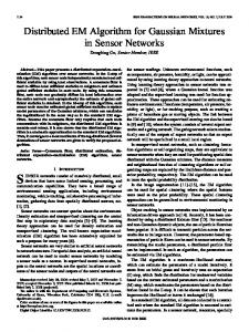
The performances of EM, SAGE and CEMM, in terms of speed, are compared on the basis of the cycles number needed to reach the stationary value of the constraint log-likelihood. ——————Figure 1 about here ——————A cycle corresponds to the updating of all mixture components. For EM, it consists of a E-step (7) and a M-step (8). For SAGE, it is the (J+1) iterations described in the Appendix. For CEMM, it consists of J iterations described in (11) and (12). In each case, a cycle of iterations requires the same number of algebraic operations ,namely, J updatings of the mixing proportions, means and variance matrices and J × n updatings of the conditional probabilities tij (θ). Figure 1 displays the log-likelihood versus cycle for EM, SAGE and CEMM in the well-separated mixture case. As expected, when starting from a good initial position in a well separated mixture situation, EM

12

converges rapidly to a local maximum of the likelihood. Moreover, EM outperforms SAGE and CEMM in this example. For the overlapping mixture, we consider two different samples of size n = 300 and performed the EM, SAGE and CEMM algorithms from the following initial position: p01 = p02 = p03 = 1/3, µ01 = 0.0, µ02 = 0.1, µ03 = 0.2, σ10 = σ20 = σ30 = 1.0, which is far from the true parameter values. For the first sample, the three algorithms converge to the same solution pˆ1

=

0.65, µ ˆ 1 = 0.85, σ ˆ 12 = 1.28

pˆ2

=

0.19, µ ˆ 2 = 3.32, σ ˆ 22 = 0.26

pˆ3

=

0.16, µ ˆ 3 = 5.67, σ ˆ 32 = 2.10. ————————–

Figures 2 and 3 about here ————————– Figure 2 displays the log-likelihood versus cycle for EM, SAGE and CEMM for the first sample of the overlapping mixture. In this situation, EM appears to converge slowly so that SAGE and especially CEMM show a significant improvement of convergence speed. For the second sample, starting from the same position, SAGE and CEMM both converge to the solution below pˆ1

=

0.61, µ ˆ 1 = 0.85, σ ˆ 12 = 1.62

pˆ2

=

0.13, µ ˆ 2 = 3.00, σ ˆ 22 = 0.52

pˆ3

=

0.26, µ ˆ 3 = 4.27, σ ˆ 32 = 4.29,

while EM proposes the following solution, after 1000 cycles, pˆ1

=

0.61, µ ˆ 1 = 0.83, σ ˆ 12 = 1.60

pˆ2

=

0.16, µ ˆ 2 = 2.98, σ ˆ 22 = 0.62

pˆ3

=

0.22, µ ˆ 3 = 4.58, σ ˆ 32 = 4.29. 13

Figure 3 displays the log-likelihood versus cycle for EM, SAGE and CEMM for the second sample of the overlapping mixture. The same conclusions hold for this sample. The CEMM algorithm is the faster while EM is really slow, the correspondant local maximum of the likelihood not being reached after 1000 ierations. Moreover, it appears that the implemented version of the SAGE algorithm is less beneficial than CEMM for situations in which EM converges slowly. A possible reason for this behavior of SAGE is that the (J + 1)th iteration of SAGE involves the whole complete data structure, whereas CEMM iterations never need the whole complete data space as missing data space.

5

Concluding remarks

We presented a component-wise EM algorithm for finite identifiable mixtures of distributions (CEMM) and proved convergence properties similar to that of standard EM. As illustrated in section 4, numerical experiments suggest that CEMM and EM have complementary performances. The CEMM algorithm is of poor interest when EM convergence is fast but shows significant improvement when EM encounters slow convergence rate. Thus, CEMM may be useful in many contexts. An intuitive explanation of our procedure performances is that the component-wise strategy prevents the algorithm from staying too long at critical points (typically saddle points) where standard EM is likely to get trapped. More theoretical investigations would be interesting but are beyond the scope of the present paper. Other futur directions of research include the use of relaxation, as in Chr´etien and Hero (1998b), for accelerating CEMM, and the possibility of using varying/adaptative orders to update the components.

14

A

Proof of Theorem 1

B

Proof of Theorem 2

n o P Let θ∗ be an accumulation point of {θk }k∈N . Note that θ∗ lies in Θ′ = θ ∈ Θ | Jℓ=1 pℓ = 1 . Take any

vector δ such that θ∗ + δ lies in Θ′ . Since Θ′ is affine, an y point θt = θ∗ + tδ, t ∈ R also lies in Θ′ . The directional derivative of Λ at θ∗ in the direction δ is obviously null. It is given by (0 =)Λ′ (θ∗ ; δ | y) = lim

t→0+

Λ(θ∗ | y) − Λ(θ∗ + tδ | y) , t

which is equal to Λ′ (θ∗ ; δ | y) = lim+ t→0

where c(θ) = n we obtain

P

J ℓ=1

L(θ∗ | y) − L(θ∗ + tδ | y) + c(θ∗ ) − c(θ∗ + tδ) , t

 pℓ − 1 . Since θ∗ + tδ lies in Θ′ for all nonnegative t, c(θ∗ + tδ) = c(θ∗ ) = 0, and Λ′ (θ∗ ; δ | y) = L′ (θ∗ ; δ | y).

Thus, L′ (θ∗ ; δ | y) = 0

(23)

References Celeux, G., Chr´etien, S., Forbes, F., and Mkhadri, A. (1999), ”A Component-Wise EM Algorithm for Mixtures”, Technical Report, Inria 3746. (http://www.inria.fr/RRRT/publications-fra.html). Chr´etien, S., and Hero, A. O.(1998a), ”Acceleration of the EM algorithm via proximal point iterations”, IEEE International Symposium on Information Theory, MIT Boston. Chr´etien, S. and Hero, A. O. (1998b), ”Generalized proximal point algorithms and bundle implementation”, Technical Report, CSPL 313, The University of Michigan, Ann Arbor, USA.

15

Chr´etien, S., and Hero, A. O. (1999), ”Kullback proximal algorithms for maximum likelihood estimation”, Technical Report, Inria 3756. (http://www.inria.fr/RRRT/publications-fra.html). Ciarlet, P. G. (1988), ”Introduction to numerical linear algebra and optimization”, Cambridge Texts in Applied Mathematics: Cambridge University Press. Dempster, A. P., Laird, N. M., and Rubin, D. B. (1977), ”Maximum likelihood for incomplete data via the EM algorithm (with discussion)”,J. Roy. Stat. Soc. Ser. B, 39, 1-38. Fessler, J. A., and Hero, A. O.(1994), ”Space-Alternating generalized expectation-maximisation algorithm”, IEEE Trans. Signal Processing, 42, 2664-2677. Fessler, J. A., and Hero, A. O. (1995), ”Penalized maximum-likelihood image reconstruction using spaceAlternating generalized EM algorithms”, IEEE Trans. Image Processing, 4, 1417-1429. Hathaway, R.J. (1986), ”Another interpretation of EM algorithm for mixture distributions”, Statist. and Probab. Letters, 4, 53-56. Hero, A. O., and Fessler, J. A. (1995), ”Convergence in norm for EM-type algorithms”, Statistica Sinica, 5, 41-54. Ibragimov, I. A., and Khas’minskij, R. Z. (1981), ”Asymptotic theory of estimation”, Springer-Verlag. Jamshidian, M. and Jennrich, R. I.”, ”Conjugate gradient acceleration of the EM algorithm”, J. Amer. Stat. Ass., 88, 221-228. Kaufman, L. (1987), ”Implementing and accelerating the EM algorithm for positron emission tomography”, IEEE Trans. Medical Image, 6, 37-51. Lewitt, R. M., and Muehllehner (1986), ”Accelerated iterative reconstruction for positron emission tomography based on the EM algorithm for maximum likelihood estimation”,IEEE Trans. on Medical Image, 5, 16-22. Liu, C., and Rubin, D.B. (1994), The ECME algorithm: A simple extension of EM and ECM with faster monotone convergence”, Biometrika, 81, 633-648. 16

Liu, C., and Sun, D. X. (1997), ”Acceleration of EM algorithm for mixtures models using ECME”, ASA Proceedings of The Stat. Comp. Session, 109-114. Liu, C., Rubin, D.B., and Wu, Y. (1998), ”Parameter expansion to accelerate EM: the PX-EM algorithm”, Biometrika, 755-770. Louis, T. A. (1982), ”Finding the observed information matrix when using the EM algorithm”, J. Roy. Stat. Soc. Ser. B, 44, 226-233. McLachlan, G. J., and Krishnam, T.(1997), ”The EM algorithm and extensions”, New York-London. Sydney-Toronto: John Wiley and Sons, Inc. Meilijson, I. (1989), ”A fast improvement to the EM algorithm in its own terms”,J. Roy. Stat. Soc. Ser. B, 51, 127-138. Meng, X.-L., and Rubin, D.B., (1993). Maximum likelihood estimation via the ECM algorithm: A general framework, Biometrika, 80, 267-278. Meng, X.-L., and van Dyk, D. A. (1997), ”The EM algorithm - an old folk song sung to a fast new tune (with discussion)”, J. Roy. Stat. Soc. Ser. B, 59, 511-567. Meng, X.-L., and van Dyk, D. A. (1998), ”Fast EM-type implementations for mixed effects models”,J. Roy. Stat. Soc. Ser. B, 60, 559-578. Neal, R. N., and Hinton, G. E. (1998), ”A view of the EM algorithm that justifies incremental, sparse and other variants”, Learning in Graphical Models, Jordan, M.I. (Editor), Dordrencht, Kluwer Academic Publishers. Pilla, R. S., and Lindsay, B. G. (1996),”Faster EM methods in high-dimensional finite mixtures”, In ”Proceedinds of the Statistical Computing Section, 166-171, Alexandria, Virginia. ASA. Redner, R. A., and Walker, H. F. (1984), ”Mixture densities, maximum likelihood and the EM algorithm”,SIAM Review, 26, 195-239. Rockafellar, R. T. (1976a), ”Augmented Lagrangians and application of the proximal point algorithm in convex programming”, Mathematics of Operations Research, 17, 96-116. 17

Rockafellar, R. T. (1976b), ”Monotone operators and the proximal point algorithm”, SIAM Journal on Control and Optimization, 14, 877-898. Teboulle, M.(1992), ”Entropic proximal mappings with application to nonlinear programming”, Mathematics of Operations Research, 17, 670-690. Teboulle, M. (1997), ”Convergence of proximal-like algorithms”, SIAM Journal on Control and Optimization, 7, 1069-1083.

18

Figure 1: Comparison of log-likelihood versus cycle for EM (full line), SAGE (dashed line) and CEMM (dotted line) in the well-separated mixture case.

Figure 2: Comparison of log-likelihood versus cycle for EM (full line), SAGE (dashed line) and CEMM (dotted line) in the overlapping mixture case (first sample).

19

Figure 3: Comparison of log-likelihood versus cycle for EM (full line), SAGE (dashed line) and CEMM (dotted line) in the overlapping mixture case (second sample).

20