1964 Greenberg; Han and Nambu: introduction of color quantum number and ... 1986 â Van Dyck, Schwinberg and Dehmelt [83]: high precision mea- surement of ..... However, a mass term for the gauge bosons like. Aa. µAa µ â (Aa. µ â. 1 g.
IFT–P/010/2000
arXiv:hep-ph/0001283v1 27 Jan 2000
Standard Model: An Introduction
∗
S. F. Novaes Instituto de F´ısica Te´orica Universidade Estadual Paulista ˜ Paulo Rua Pamplona 145, 01405–900, Sao Brazil
Abstract
We present a primer on the Standard Model of the electroweak interaction. Emphasis is given to the historical aspects of the theory’s formulation. The radiative corrections to the Standard Model are presented and its predictions for the electroweak parameters are compared with the precise experimental data obtained at the Z pole. Finally, we make some remarks on the perspectives for the discovery of the Higgs boson, the most important challenge of the Standard Model.
∗
To be published in Particle and Fields, Proceedings of the X J. A. Swieca Summer School (World Scientific, Singapore, 2000)
Contents 1 Introduction
4
1.1 A Chronology of the Weak Interactions . . . . . . . . . . .
6
1.2 The Gauge Principle . . . . . . . . . . . . . . . . . . . . .
18
1.2.1 Gauge Invariance in Quantum Mechanics . . . . .
19
1.2.2 Gauge Invariance for Non–Abelian Groups . . . .
22
1.3 Spontaneous Symmetry Breaking . . . . . . . . . . . . . .
25
1.4 The Higgs Mechanism . . . . . . . . . . . . . . . . . . . .
31
1.4.1 The Abelian Higgs Mechanism . . . . . . . . . . .
31
1.4.2 The Non–Abelian Case . . . . . . . . . . . . . . . .
34
2 The Standard Model
35
2.1 Constructing the Model . . . . . . . . . . . . . . . . . . . .
35
2.1.1 General Principles to Construct Gauge Theories .
35
2.1.2 Right– and Left– Handed Fermions . . . . . . . .
37
2.1.3 Choosing the gauge group . . . . . . . . . . . . . .
38
2.1.4 The Higgs Mechanism and the W and Z mass . .
44
2.2 Some General Remarks . . . . . . . . . . . . . . . . . . . .
48
2.2.1 On the mass matrix of the neutral bosons . . . . .
48
2.2.2 On the ρ Parameter . . . . . . . . . . . . . . . . . .
48
2.2.3 On the Gauge Fixing Term . . . . . . . . . . . . . .
49
2
3
4
2.2.4 On the Measurement of sin2 θW at Low Energies .
51
2.2.5 On the Lepton Mass . . . . . . . . . . . . . . . . .
52
2.2.6 On the Cross Sections e+ e− → W + W − . . . . . . .
53
2.3 Introducing the Quarks . . . . . . . . . . . . . . . . . . . .
55
2.3.1 On Anomaly Cancellation . . . . . . . . . . . . . .
57
2.3.2 The Quark Masses . . . . . . . . . . . . . . . . . .
58
2.4 The Standard Model Lagrangian . . . . . . . . . . . . . .
61
Beyond the Trees
64
3.1 Radiative Corrections to the Standard Model . . . . . . .
64
3.1.1 One Loop Calculations . . . . . . . . . . . . . . . .
66
3.2 The Z boson Physics . . . . . . . . . . . . . . . . . . . . .
69
3.2.1 Introduction . . . . . . . . . . . . . . . . . . . . . .
69
3.2.2 The Standard Model Parameters . . . . . . . . . .
71
The Higgs Boson Physics
81
4.1 Introduction . . . . . . . . . . . . . . . . . . . . . . . . . .
81
4.2 Higgs Boson Properties . . . . . . . . . . . . . . . . . . . .
82
4.3 Production and Decay Modes . . . . . . . . . . . . . . . .
87
4.3.1 The Decay Modes of the Higgs Boson . . . . . . . .
87
4.3.2 Production Mechanisms at Colliders . . . . . . . .
89
5 Closing Remarks
91
References
93
3
Chapter 1 Introduction The joint description of the electromagnetic and the weak interaction by a single theory certainly is one of major achievements of the physical science in this century. The model proposed by Glashow, Salam and Weinberg in the middle sixties, has been extensively tested during the last 30 years. The discovery of neutral weak interactions and the production of intermediate vector bosons (W ± and Z 0 ) with the expected properties increased our confidence in the model. Even after the recent precise measurements of the electroweak parameters in electron–positron collisions at the Z 0 pole, there is no experimental result that contradicts the Standard Model predictions. The description of the electroweak interaction is implemented by a gauge theory based on the SU(2)L ⊗ U(1)Y group, which is spontaneously broken via the Higgs mechanism. The matter fields — leptons and quarks — are organized in families, with the left–handed fermions belonging to weak isodoublets while the right–handed components transform as weak isosinglets. The vector bosons, W ± , Z 0 and γ, that mediate the interactions are introduced via minimal coupling to the matter fields. An essential ingredient of the model is the scalar potential that is added to the Lagrangian to generate the vector–boson (and fermion) masses in a gauge invariant way, via the Higgs mechanism. A remnant scalar field, the Higgs boson, is part of the physical spectrum. This is the only missing piece of the Standard Model that still awaits experimental confirmation. 4
In this course, we intend to give a quite pedestrian introduction to the main concepts involved in the construction of the Standard Model of electroweak interactions. We should not touch any subject “beyond the Standard Model”. This primer should provide the necessary background for the lectures on more advanced topics that were covered in this school, such as W physics and extensions of the Standard Model. A special emphasis will be given to the historical aspects of the formulation of the theory. The interplay of new ideas and experimental results make the history of weak interactions a very fruitful laboratory for understanding how the development of a scientific theory works in practice. More formal aspects and details of the model can be found in the vast literature on this subject, from textbooks [1, 2, 3, 4, 5, 6, 7] to reviews [8, 9, 10, 11]. We start these lectures with a chronological account of the ideas related to the development of electromagnetic and weak theories (Section 1.1). The gauge principle (Sec. 1.2) and the concepts of spontaneous symmetry breaking (Sec. 1.3) and the Higgs mechanism (Section 1.4) are presented. In the Chapter 2, we introduce the Standard Model, following the general principles that should guide the construction of a gauge theory. We discuss topics like the mass matrix of the neutral bosons, the measurement of the Weinberg angle, the lepton mass, anomaly cancelation, and the introduction of quarks in the model. We finalize this chapter giving an overview on the Standard Model Lagrangian in Sec. 2.4. In Chapter 3, we give an introduction to the radiative corrections to the Standard Model. Loop calculations are important to compare the predictions of the Standard Model with the precise experimental results of Z physics that are presented in Sec. 3.2. We finish our lectures with an account on the most important challenge to the Standard Model: the discovery of the Higgs boson. In Chapter 4, we discuss the main properties of the Higgs, like mass, couplings and decay modes and discuss the phenomenological prospects for the search of the Higgs in different colliders. Most of the material covered in these lectures can be found in a series of very good textbook on the subject. Among them we can point out the books from Quigg [1], Aitchison and Hey [4], and Leader and Predazzi [7].
5
1.1
A Chronology of the Weak Interactions
We will present in this section the main steps given towards a unified description of the electromagnetic and weak interactions. In order to give a historical flavor to the presentation, we will mention some parallel achievements in Particle Physics in this century, from theoretical developments and predictions to experimental confirmation and surprises. The topics closely related to the evolution and construction of the model will be worked with more details. The chronology of the developments and discoveries in Particle Physics can be found in the books of Cahn and Goldhaber [12] and the annotated bibliography from COMPAS and Particle Data Groups [13]. An extensive selection of original papers on Quantum Electrodynamics can be found in the book edited by Schwinger [14]. Original papers on gauge theory of weak and electromagnetic interactions appear in Ref. [15].
1896 ⋆ Becquerel [16]: evidence for spontaneous radioactivity effect in uranium decay, using photographic film. 1897
⋆
Thomson: discovery of the electron in cathode rays.
1900
⋆
Planck: start of the quantum era.
1905 Einstein: start of the relativistic era. 1911
⋆
Millikan: measurement of the electron charge.
1911 Rutherford: evidence for the atomic nucleus. 1913
⋆
Bohr: invention of the quantum theory of atomic spectra.
1914 Chadwick [17]: first observation that the β spectrum is continuous. Indirect evidence on the existence of neutral penetrating particles. 1919 Rutherford: discovery of the proton, constituent of the nucleus. 1923 ⋆ Compton: experimental confirmation that the photon is an elementary particle in γ + C → γ + C. The “star” (⋆) means that the author(s) have received the Nobel Prize in Physics for this particular work. ⋆
6
1923
⋆
de Broglie: corpuscular–wave dualism for electrons.
1925
⋆
Pauli: discovery of the exclusion principle.
1925
⋆
Heisenberg: foundation of quantum mechanics.
1926
⋆
Schr¨odinger: creation of wave quantum mechanics.
1927 Ellis and Wooster [18]: confirmation that the β spectrum is continuous. 1927 Dirac [19]: foundations of Quantum Electrodynamics (QED). 1928 ⋆ Dirac: discovery of the relativistic wave equation for electrons; prediction of the magnetic moment of the electron. 1929 Skobelzyn: observation of cosmic ray showers produced by energetic electrons in a cloud chamber. 1930 Pauli [20]: first proposal, in an open letter, of the existence of a light, neutral and feebly interacting particle emitted in β decay. 1930 Oppenheimer [21]: self–energy of the electron: the first ultraviolet divergence in QED. 1931 Dirac: prediction of the positron and anti–proton. 1932
⋆
Anderson: first evidence for the positron.
1932
⋆
Chadwick: first evidence for the neutron in α + Be → C + n.
1932 Heisenberg: suggestion that nuclei are composed of protons and neutrons. 1934 Pauli [22]: explanation of continuous electron spectrum of β decay — proposal for the neutrino. n → p + e− + ν¯e .
1934 Fermi [23]: field theory for β decay, assuming the existence of the neutrino. In analogy to “the theory of radiation that describes the emission of a quantum of light from an excited atom”, eJµ Aµ , Fermi proposed a current–current Lagrangian to describe the β decay: � � GF Lweak = √ ψ¯p γµ ψn ψ¯e γ µ ψν . 2 7
1936 Gamow and Teller [24]: proposed an extension of the Fermi theory to describe also transitions with ∆J nuc 6= 0. The vector currents proposed by Fermi are generalized to: � � GF X Lweak = √ Ci ψ¯p Γi ψn ψ¯e Γi ψν , 2 i with the scalar, pseudo–scalar, vector, axial and tensor structures: ΓS = 1 , ΓP = γ 5 ,
ΓVµ = γµ , ΓA µ = γµ γ5 ,
ΓTµν = σµν .
Nuclear transitions with ∆J = 0 are described by the interactions S.S and/or V.V , while ∆J = 0, ±1 (0 6→ 0) transitions can be taken into account by A.A and/or T.T interactions (ΓP → 0 in the non–relativistic limit). However, interference between them are proportional to me /Ee and should increase the emission of low energy electrons. Since this behavior was not observed, the weak Lagrangian should contain, S.S or V.V
and A.A or T.T .
1937 Neddermeyer and Anderson: first evidence for the muon. 1937 Majorana: Majorana neutrino theory. 1937 Bloch and Nordsieck [25]: treatment of infrared divergences. 1940 Williams and Roberts [26]: first observation of muon decay µ− → e− + (¯ νe + νµ ) .
1943 Heisenberg: invention of the S–matrix formalism. 1943 ⋆ Tomonaga [27]: creation of the covariant quantum electrodynamic theory. 1947 Pontecorvo [28]: first idea about the universality of the Fermi weak interactions i.e. decay and capture processes have the same origin. 1947 Bethe [29]: first theoretical calculation of the Lamb shift in non– relativistic QED. 8
1947 ⋆ Kusch and Foley [30]: first measurement of ge − 2 for the electron using the Zeeman effect: ge = 2(1 + 1.19 × 10⁻³ ).
1947 ⋆ Lattes, Occhialini and Powell: confirmation of the π − and first evidence for pion decay π ± → µ± + (νµ ). 1947 Rochester and Butler: first evidence for V events (strange particles).
1948 Schwinger [31]: first theoretical calculation of ge − 2 for the electron: ge = 2(1 + α/2π) = 2(1 + 1.16 × 10⁻³). The high–precision measurement of the anomalous magnetic moment of the electron is the most stringent QED test. The present theoretical and experimental value of ae = (ge − 2)/2, are [32], athr = (115 965 215.4 ± 2.4) × 10−11 , e aexp = (115 965 219.3 ± 1.0) × 10−11 , e where we notice the impressive agreement at the 9 digit level!
1948 ⋆ Feynman [33]; Schwinger [34]; Tati and Tomonaga [35]: creation of the covariant theory of QED. 1949 Dyson [36]: covariant QED and equivalence of Tomonaga, Schwinger and Feynman methods. 1949 Wheeler and Tiomno [37]; Lee, Rosenbluth and Yang [38]: proposal of the universality of the Fermi weak interactions. Different processes like, β − decay µ − decay µ − capture
: : :
n → p + e− + ν¯e , µ− → e− + ν¯e + νµ , µ− + p → νµ + n ,
must have the same nature and should share the same coupling constant, GF =
1.03 × 10⁻⁵ , Mp2
the so–called Fermi constant.
50’s A large number of new particles where discovered in the 50’s: π 0 , ¯ Ξ0 , · · · K ± , Λ, K 0 , ∆++ , Ξ− , Σ± , ν¯e , p¯, KL,S , n ¯ , Σ0 , Λ, 9
1950 Ward [39]: Ward identity in QED. ¨ 1953 Stuckelberg; Gell–Mann: invention and exploration of renormalization group.
1954 Yang and Mills [40]: introduction of local gauge isotopic invariance in quantum field theory. This was one of the key theoretical developments that lead to the invention of non–abelian gauge theories. 1955 Alvarez and Goldhaber [41]; Birge et al. [42]: θ − τ puzzle: The “two” particles seem to be a single state since they have the same width (Γθ = Γτ ), and the same mass (Mθ = Mτ ). However the observation of different decay modes, into states with opposite parity: θ+ → π + + π 0 , J P = 0+ , τ + → π + + π + + π − , J P = 0− , suggested that parity could be violated in weak transitions.
1955 Lehmann, Symanzik and Zimmermann: beginnings of the axiomatic field theory of the S–matrix. 1955 Nishijima: classification of strange particles and prediction of Σ0 and Ξ0 . 1956 ⋆ Lee and Yang [43]: proposals to test spatial parity conservation in weak interactions. 1957 Wu et al. [44]: obtained the first evidence for parity nonconservation in weak decays. They measured the angular distribution of the electrons in β decay, 60
Co (polarized) →
60
Ni + e− + ν¯e ,
and observed that the decay rate depend on the pseudo–scalar quantity: < J~nuc > . ~pe .
1957 Garwin, Lederman and Weinrich [45]; Friedman and Telegdi [46]: confirmation of parity violation in weak decays. They make the measurement of the electron asymmetry (muon polarization) in the decay chain, π + → µ+ + νµ ֒→ e+ + νe + ν¯µ . 10
1957 Frauenfelder et al. [47]: further confirmation of parity nonconservation in weak decays. The measurement of the longitudinal polarization of the electron (~σe .~pe ) emitted in β decay, 60
Co → e− (long. polar.) + ν¯e + X ,
showed that the electrons emitted in weak transitions are mostly left– handed. The confirmation of the parity violation by the weak interaction showed that it is necessary to have a term containing a γ5 in the weak current: �� � GF X Lweak → √ Ci ψ¯p Γi ψn ψ¯e Γi (1 ± γ5 ) ψν . 2 i Note that CP remains conserved since C is also violated.
1957 Salam [48] ; Lee and Yang [49]; Landau [50]: two–component theory of neutrino. This requires that the neutrino is either right or left–handed. Since it was known that electrons (positrons) involved in weak decays are left (right) handed, the leptonic current should be written as: � � � � (1 + γ5 ) i i i ¯ ¯ Γ (1 ± γ5 ) ψν . Jlept ≡ ψe Γ (1 ± γ5 ) ψν → ψe 2 Therefore the measurement of the neutrino helicity is crucial to determine the structure of the weak current. If Γi = V or A then {γ5 , Γi} = 0 and the neutrino should be left–handed, otherwise the current is zero. On the other hand, if Γi = S or T , then [γ5 , Γi ] = 0, and the neutrino should be right–handed.
1957 Schwinger [51]; Lee and Yang [52]: development of the idea of the intermediate vector boson in weak interaction. The four–fermion Fermi interaction is “point–like” i.e. a s–wave interaction. Partial wave unitarity requires that such interaction must give rise to a cross section that is bound by σ < 4π/p2cm . However, since GF has dimension of M −2 , the cross section for the Fermi weak interaction should go like σ ∼ G2F p2cm . Therefore the Fermi theory violates unitarity for pcm ≃ 300 GeV. 11
This violation can be delayed by imposing that the interaction is transmitted by a intermediate vector boson (IVB) in analogy, once again, with the quantum electrodynamics. Here, the IVB should have quite different characteristics, due to the properties of the weak interaction. The IVB should be charged since the β decay requires charge–changing currents. They should also be very massive to account for short range of the weak interaction and they should not have a definite parity to allow, for instance, a V − A structure for the weak current. With the introduction of the IVB, the Fermi Lagrangian for leptons, � GF � Lweak = √ J α (ℓ)Jα† (ℓ′ ) + h.c. , 2
where J α (ℓ) = ψ¯νℓ Γα ψℓ , becomes:
� α + †α LW Wα− , weak = GW J Wα + J
(1.1)
with a new coupling constant GW .
Let us compare the invariant amplitude for µ–decay, in the low– energy limit in both cases. For the Fermi Lagrangian, we have, GF Mweak = i √ J α (µ)Jα (e) . 2
(1.2)
On the other hand, when we take into account the exchange of the IVB, the invariant amplitude should include the vector boson propagator, � � �� � � −i kα kβ W α β Mweak = [i GW J (µ)] 2 g − i G J (e) . αβ W 2 2 k − MW MW
2 At low energies, i.e. for k 2 ≪ MW ,
MW weak
G2W α −→ i 2 J (µ)Jα (e) , MW
(1.3)
and, comparing (1.3) with (1.2) we obtain the relation G2W =
2 MW G √ F 2
12
,
(1.4)
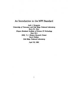
which shows that GW is dimensionless. However, at high energies, the theory of IVB still violates unitarity, for instance, in the cross section for ν ν¯ → W + W − (see Fig. 1).
Let us consider the W ± polarization states. At the W ± rest frame, we can define the transversal and longitudinal polarizations as ǫµT1 (0) = (0, 1, 0, 0) , ǫµT2 (0) = (0, 0, 1, 0) , ǫµL (0) = (0, 0, 0, 1) .
neutrino
W+ electron W-
antineutrino
Fig. 1: Feynman diagram for the process ν + ν¯ → W + + W − . After a boost along the z direction, i.e. transversal states remain unchanged while comes, � � |~p| E µ , pˆ ≃ ǫL (p) = MW MW
for pµ = (E, 0, 0, p), the the longitudinal state bepµ . MW
Since the longitudinal polarization is proportional to the vector boson momentum, at high energies the longitudinal amplitudes should give rise to the worst behavior. In fact, in high energy limit, the polarized cross section for ν ν¯ → W W − behaves like, +
σ(ν ν¯ → WT+ WT− ) −→ constant G2F s σ(ν ν¯ → WL+ WL− ) −→ , 3π 13
which still violates unitarity for large values of s.
1958 Feynman and Gell–Mann [53]; Marshak and Sudarshan [54]; Sakurai [55]: universal V − A weak interactions. � � +µ Jlept = ψ¯e γ µ (1 − γ5 ) ψν . (1.5)
1958 Leite Lopes [56]: hypothesis of neutral vector mesons exchanged in weak interaction. Prediction of its mass of ∼ 60 mproton .
1958 Goldhaber, Grodzins and Sunyar [57]: first evidence for the negative νe helicity. As mentioned before, this result requires that the structure of the weak interaction is V − A. 1959 ⋆ Reines and Cowan: confirmation of the detection of the ν¯e in ν¯e + p → e+ + n.
1961 Goldstone [58]: prediction of unavoidable massless bosons if global symmetry of the Lagrangian is spontaneously broken. 1961 Salam and Ward [59]: invention of the gauge principle as basis to construct quantum field theories of interacting fundamental fields. 1961 ⋆ Glashow [60]: first introduction of the neutral intermediate weak boson (Z 0 ). 1962
⋆
Danby et al.: first evidence of νµ from π ± → µ± + (ν/¯ ν ).
1963 Cabibbo [61]: introduction of the Cabibbo angle and hadronic weak currents. It was observed experimentally that weak decays with change of strangeness (∆s = 1) are strongly suppressed in nature. For instance, the width of the neutron is much larger than the Λ’s, Γ∆s=0 (nudd → puud e¯ ν ) ≫ Γ∆s=1 (Λuds → puud e¯ ν) , which yield a branching ratio of 100% in the case of neutron and just ∼ 8 × 10⁻⁴ for the Λ.
The hadronic current, in analogy with leptonic current (1.5), can be written in terms of the u, d, and s quarks, ¯ µ (1 − γ5 )u + s¯γµ (1 − γ5 )u , JµH = dγ 14
(1.6)
where the first term is responsible for the ∆s = 0 transitions while the latter one gives rise to the ∆s = 1 processes. In order to make the hadronic current also universal, with a common coupling constant GF , Cabibbo introduced a mixing angle to give the right weight to the ∆s = 0 and ∆s = 1 parts of the hadronic current, �� � � � ′ � d cos θC sin θC d , (1.7) = s − sin θC cos θC s′ where d′ , s′ (d, s) are interaction (mass) eigenstates. Now the transition d¯ ↔ u is proportional to GF cos θC ≃ 0.97 GF and the s¯ ↔ u goes like GF sin θC ≃ 0.24 GF .
The hadronic current should now be given in terms of the new interaction eigenstates, JµH = d¯′ γµ (1 − γ5 )u ¯ µ (1 − γ5 )u + sin θC s¯γµ (1 − γ5 )u . = cos θC dγ
(1.8)
1964 Bjorken and Glashow [62]: proposal for the existence of a charmed fundamental fermion (c). 1964 Higgs [63]; Englert and Brout [64]; Guralnik, Hagen and Kibble [65]: example of a field theory with spontaneous symmetry breakdown, no massless Goldstone boson, and massive vector boson. 1964 ⋆ Christenson, Cronin, Fitch and Turlay [66]: first evidence of CP violation in the decay of K 0 mesons. 1964 ⋆ Salam and Ward [67]: Lagrangian for the electroweak synthesis, estimation of the W mass. 1964 ⋆ Gell–Mann; Zweig: introduction of quarks as fundamental building blocks for hadrons. 1964 Greenberg; Han and Nambu: introduction of color quantum number and colored quarks and gluons. 1967 Kibble [68]: extension of the Higgs mechanism of mass generation for non–abelian gauge field theories. 1967 ⋆ Weinberg [69]: Lagrangian for the electroweak synthesis and estimation of W and Z masses. 15
1967 Faddeev and Popov [70]: method for construction of Feynman rules for Yang–Mills gauge theories. 1968
⋆
Salam [71]: Lagrangian for the electroweak synthesis.
1969 Bjorken: invention of the Bjorken scaling behavior. 1969 Feynman: birth of the partonic picture of hadron collisions. 1970 Glashow, Iliopoulos and Maiani [72]: introduction of lepton– quark symmetry and the proposal of charmed quark (GIM mechanism). 1971 ⋆ ’t Hooft [73]: rigorous proof of renormalizability of the massless and massive Yang– Mills quantum field theory with spontaneously broken gauge invariance. 1973 Kobayashi and Maskawa [74]: CP violation is accommodated in the Standard Model with six favours. 1973 Hasert et al. (CERN) [75]: first experimental indication of the existence of weak neutral currents. ν¯µ + e− → ν¯µ + e− ,
νµ + N → νµ + X .
This was a dramatic prediction of the Standard Model and its discovery was a major success for the model. They also measured the ratio of neutral–current to charged–current events giving a estimate for the Weinberg angle sin2 θW in the range 0.3 to 0.4.
1973 Gross and Wilczek; Politzer: discovery of asymptotic freedom property of interacting Yang–Mills field theories. 1973 Fritzsch, Gell–Mann and Leutwyler: invention of the QCD Lagrangian. 1974 Benvenuti et al. (Fermilab) [76]: confirmation of the existence of weak neutral currents in the reaction νµ + N → νµ + X .
1974 ⋆ Aubert et al. (Brookhaven); Augustin et al. (SLAC): evidence for the J/ψ (c¯ c). 1975
⋆
Perl et al. (SLAC) [77]: first indication of the τ lepton.
1977 Herb et al. (Fermilab) [78]: first evidence of Υ (b¯b). 16
1979 Barber et al. (MARK J Collab.); Brandelik et al. (TASSO Collab.); Berger et al. (PLUTO Collab.); W. Bartel (JADE Collab.): evidence for the gluon jet in e+ e− → 3 jet.
1983 ⋆ Arnison et al. (UA1 Collab.) [79]; Banner et al. (UA2 Collab.) [80]: evidence for the charged intermediate bosons W ± in the reactions p + p¯ → W (→ ℓ + ν) + X . They were able to estimate the W boson mass (MW = 81 ± 5 GeV) in good agreement with the predictions of the Standard Model.
1983 ⋆ Arnison et al. (UA1 Collab.) [81]; Bagnaia et al. (UA2 Collab.) [82]: evidence for the neutral intermediate boson Z 0 in the reaction p + p¯ → Z(→ ℓ+ + ℓ− ) + X . This was another important confirmation of the electroweak theory.
1986 ⋆ Van Dyck, Schwinberg and Dehmelt [83]: high precision measurement of the electron ge − 2 factor. ¯0 1987 Albrecht et al. (ARGUS Collab.) [84]: first evidence of B 0 − B mixing. 1989 Abrams et al. (MARK-II Collab.) [85]: first evidence that the number of light neutrinos is 3. 1992 LEP Collaborations (ALEPH, DELPHI, L3 and OPAL) [86]: precise determination of the Z 0 parameters. 1995 Abe et al. (CDF Collab.) [87]; Abachi et al. (DØ Collab.) [88]: observation of the top quark production.
17
1.2
The Gauge Principle
As it is well known, symmetry has always played a very important rˆole in the development of physics. From the spacetime symmetry of special relativity, up to the internal and gauge invariances, the symmetries have mapped out the route to most of the physical theories in this last century. An important result for field theory and particle physics is provided by the Noether’s theorem. If an action is invariant under some group of transformations (symmetry), then there exist one or more conserved quantities (constants of motion) which are associated to these transformations. In this sense, Noether’s theorem establishes that symmetries imply conservation laws. A natural question to ask would be: upon imposing to a given Lagrangian the invariance under a certain symmetry, would it be possible to determine the form of the interaction among the particles? In other words, could symmetry also imply dynamics? In fact, this happens in Quantum Electrodynamics (QED), the best theory ever built to describe Nature, which had become a prototype of a successful quantum field theory. In QED the existence and some of the properties of the gauge field — the photon — follow from a principle of invariance under local gauge transformations of the U(1) group. Could this principle be generalized to other interactions? For Salam and Ward [59], who invented the gauge principle as the basis to construct the quantum field theory of interacting fields, this was a possible dream: “Our basic postulate is that it should be possible to generate strong, weak and electromagnetic interaction terms (with all their correct symmetry properties and also with clues regarding their relative strengths) by making local gauge transformations on the kinetic–energy terms in the free Lagrangian for all particles.” In fact, those ideas could be accomplished just after some new and important ingredients were introduced to describe short distance (weak) 18
and strong interactions. In the case of weak interactions the presence of very heavy weak gauge bosons require the new concept of spontaneous breakdown of the gauge symmetry and the Higgs mechanism [63, 64, 65]. On the other hand, the concept of asymptotic freedom [89, 90] played a crucial rˆole to describe perturbatively the strong interaction at short distances, making the strong gauge bosons trapped. The Quantum Chromodynamics (QCD), the gauge theory for strong interactions, is the subject of Mangano’s lecture at this school.
1.2.1 Gauge Invariance in Quantum Mechanics The gauge principle and the concept of gauge invariance are already present in Quantum Mechanics of a particle in the presence of an electromagnetic field [4]. Let us start from the classical Hamiltonian that ~ + q~v × B), ~ gives rise to the Lorentz force (F~ = q E �2 1 � ~ + qφ , H= p~ − q A (1.9) 2m where the electric and magnetic fields can be described in terms of the ~ potentials Aµ = (φ, A), ~ ~ =∇ ~ ×A ~. ~ = −∇φ ~ − ∂A ; , B E ∂t These fields remain exactly the same when we make the gauge transformation (G) in the potentials: φ → φ′ = φ −
∂χ , ∂t
~→A ~′ = A ~ + ∇χ ~ . A
(1.10)
When we quantize the Hamiltonian (1.9) by applying the usual pre~ we get the Schr¨odinger equation for a particle in an scription ~p → −i∇, electromagnetic field, � � �2 ∂ψ(x, t) 1 � ~ ~ −i∇ − q A + qφ ψ(x, t) = i , 2m ∂t
which can be written in a compact form as
1 ~ 2 ψ = iD0 ψ , (−iD) 2m 19
(1.11)
The equation (1.11) is equivalent to make the substitution ∂ ∂ ~ →D ~ =∇ ~ − iq A ~ , ∇ → D0 = + iqφ . ∂t ∂t in the free Schr¨odinger equation. G ~ −→ ~ ′ ), given by If we make the gauge transformation, (φ, A) (φ′ , A ′ (1.10), does the new field ψ which is solution of 1 ~ ′ )2 ψ ′ = iD ′ ψ ′ , (−iD 0 2m describe the same physics?
The answer to this question is no. However, we can recover the invariance of our theory by making, at the same time, the phase transformation in the matter field ψ ′ = exp (iqχ) ψ
(1.12)
with the same function χ = χ(x, t) used in the transformation of electromagnetic fields (1.10). The derivative of ψ ′ transforms as, h i ′ ′ ~ ~ ~ ~ D ψ = ∇ − iq(A + ∇χ) exp (iqχ) ψ ~ ~ exp (iqχ) ψ = exp (iqχ) (∇ψ)+iq( ∇χ) ~ exp (iqχ) ψ−iq(∇χ) ~ exp (iqχ) ψ −iq A ~ , = exp (iqχ) Dψ
(1.13)
and in the same way, we have for D0 , D0′ ψ ′ = exp (iqχ) D0 ψ .
(1.14)
We should mention that now the field ψ (1.12) and its derivatives ~ (1.13), and D0 ψ (1.14), all transform exactly in the same way: they Dψ are all multiplied by the same phase factor. Therefore, the Schr¨odinger equation (1.11) for ψ ′ becomes 1 ~ ′ )2 ψ ′ = 1 (−iD ~ ′ )(−iD ~ ′ ψ′) (−iD 2m 2m h i 1 ~ ′ ) −i exp (iqχ) Dψ ~ = (−iD 2m 1 ~ 2ψ (−iD) = exp (iqχ) 2m = exp (iqχ) (iD0 )ψ = iD0′ ψ ′ . 20
and now both ψ and ψ ′ describe the same physics, since |ψ|2 = |ψ ′ |2 . In order to get the invariance for all observables, we should assure that the following substitution is made: ~ →D ~ , ∇
∂ → D0 , ∂t
For instance, the current ~ ~ ∗ψ , J~ ∝ ψ ∗ (∇ψ) − (∇ψ) becomes also gauge invariant with this substitution since ~ ′ ψ ′ ) = ψ ∗ exp (−iqχ) exp (iqχ) (Dψ) ~ ~ ψ ∗ ′ (D = ψ ∗ (Dψ) . After we have shown how to obtain a gauge invariant quantum description of a particle in an electromagnetic field, could we reverse the argument? That is: when we demand that a theory is invariant under a spacetime dependent phase transformation, can this procedure impose the specific form of the interaction with the gauge field? In other words, can the symmetry imply dynamics? Let us examine what happens when we start from the Dirac free Lagrangian ¯ 6 ∂ − m)ψ , Lψ = ψ(i that is not invariant under the local gauge transformation, ψ → ψ ′ = exp [−iα(x)] ψ , since ¯ µ ψ(∂ µ α) , Lψ → L′ψ = Lψ + ψγ However, if we introduce the gauge field Aµ through the minimal coupling Dµ ≡ ∂µ + ieAµ , and, at the same time, require that Aµ transforms like 1 Aµ → A′µ = Aµ + ∂µ α . e 21
(1.15)
we have Lψ → L′ψ = ψ¯′ [(i 6 ∂ − e A 6 ′ ) − m] ψ ′ � � � � 1 ¯ 6 + 6 ∂α − m exp(−iα)ψ = ψ exp(+iα) i 6 ∂ − e A e µ ¯ = Lψ − eψγµ ψA . (1.16) The coupling between ψ (e.g. electrons) and the gauge field Aµ (photon) arises naturally when we require the invariance under local gauge transformations of the kinetic–energy terms in the free fermion Lagrangian. Since, the electromagnetic strength tensor Fµν ≡ ∂µ Aν − ∂ν Aµ ,
(1.17)
is invariant under the gauge transformation (1.15), so is the Lagrangian for free gauge field, 1 LA = − Fµν F µν , 4
(1.18)
This Lagrangian together with (1.16) describes the Quantum Electrodynamics. We should point out that a hypothetical mass term for the gauge field, 1 µ Lm A = − Aµ A , 2 is not invariant under the transformation (1.15). Therefore, something else should be necessary to describe massive vector bosons in a gauge invariant way, preserving the renormalizability of the theory.
1.2.2 Gauge Invariance for Non–Abelian Groups As suggested by Heisenberg [91] in 1932, under nuclear interactions, protons and neutron can be regarded as degenerated since their mass are quite similar and electromagnetic interaction is negligible. 22
Therefore any arbitrary combination of their wave function would be equivalent, � � ψp ψ≡ → ψ ′ = Uψ , ψn where U is unitary transformation (U † U = UU † = 1) to preserve normalization (probability). Moreover, if det|U| = 1, U represents the Lie group SU(2): � � τa a τa U = exp −i α ≃ 1 − i αa , 2 2 where τ a , a = 1, 2, 3 are the Pauli matrices. In 1954, Yang and Mills [40] introduced the idea of local gauge isotopic invariance in quantum field theory. “The differentiation between a neutron and a proton is then a purely arbitrary process. As usually conceived, however, this arbitrariness is subject to the following limitation: once one chooses what to call a proton, what a neutron, at one spacetime point, one is then not free to make any choices at other spacetime points. It seems that this is not consistent with the localized field concept that underlies the usual physical theories.” Following their argument, we should preserve our freedom to choose what to call a proton or a neutron no matter when or where we are. This can be implemented by requiring that the gauge parameters depend on the spacetime points, i.e. αa → αa (x).
This idea was generalized by Utiyama [92] in 1956 for any non– Abelian group G with generators ta satisfying the Lie algebra [8], [ta , tb ] = i Cabc tc ,
with Cabc being the structure constant of the group. The Lagrangian Lψ should be invariant under the matter field transformation ψ → ψ′ = Ω ψ , 23
with Ω ≡ exp [−i T a αa (x)] , where T a is a convenient representation (i.e. according to the fields ψ) of the generators ta . Introducing one gauge field for each generator, and defining the covariant derivative by Dµ ≡ ∂µ − igT a Aaµ , Since the covariant derivative transforms just like the matter field, i.e. Dµ ψ → Ω (Dµ ψ), this will ensure the invariance under the local non–Abelian gauge transformation for the terms containing the fields and its gradients as long as the gauge field transformation is � � i a a a a T Aµ → Ω T Aµ + ∂µ Ω−1 , g or, in infinitesimal form, i.e. for Ω ≃ 1 − i T a αa (x), 1 Aaµ ′ = Aaµ − ∂µ αa + Cabc αb Acµ . g Finally, we should generalize the strength tensor (1.17) for a non– abelian Lie group, a Fµν ≡ ∂µ Aaν − ∂ν Aaµ + g Cabc Abµ Acν ,
(1.19)
a′ a c which transforms like Fµν → Fµν + Cabc αb Fµν . Therefore, the invariant kinetic term for the gauge bosons, can be written as
1 a a µν LA = − Fµν F , 4
(1.20)
and is invariant under the local gauge transformation. However, a mass term for the gauge bosons like � �� � 1 1 a b c aµ a d eµ a aµ a , A − ∂µ α + Cade α A Aµ A → Aµ − ∂µ α + Cabc α Aµ g g 24
is still not gauge invariant. Note that since F ∝ (∂A − ∂A) + gAA , unlike the Abelian case, there is a new feature: the gauge fields have triple and quartic self–couplings, LA ∝ (∂A − ∂A)2 + g(∂A − ∂A)AA + g 2 AAAA . propagator triple quartic
1.3
Spontaneous Symmetry Breaking
Exact symmetries give rise, in general, to exact conservation laws. In this case both the Lagrangian and the vacuum (the ground state of the theory) are invariant. However, there are some conservation laws which are not exact, e.g. isospin, strangeness, etc. These situations can be described by adding to the invariant Lagrangian (Lsym ) a small term that breaks this symmetry (Lsb ), L = Lsym + ε Lsb . Another situation occurs when the system has a Lagrangian that is invariant and a non–invariant vacuum. A classic example of the situation is provided by a ferromagnet where the Lagrangian describing the spin–spin interaction is invariant under tridimensional rotations. For temperatures above the ferromagnetic transition temperature (TC ) the spin system is completely disordered (paramagnetic phase), and therefore the vacuum is also SO(3) invariant [see Fig. 2(a)]. However, for temperatures below TC (ferromagnetic phase) a spontaneous magnetisation of the system occurs, aligning the spins in some specific direction [see Fig. 2(b)]. In this case, the vacuum is not invariant under the SO(3) group. This symmetry is broken to SO(2), representing the rotation of the whole system around the spin directions.
25
−→ տ ց ↑ −→ ւ
ր ր ր ր ր ր
տ ↓ ր տ ւ ւ
ր ր ր ր ր ր
←− ր տ տ ւ ւ
ր ր ր ր ր ր
(a)
(b)
↑ −→ ւ −→ տ ց
ր ր ր ր ր ր
−→ −→ ւ տ −→ ր
ր ր ր ր ր ր
Fig. 2: Representation of the spin orientation in the paramagnetic (a) and ferromagnetic (b) phases. Let us analyze the simple example of a scalar self–interacting real field with Lagrangian, 1 L = ∂µ φ ∂ µ φ − V (φ) , 2
(1.21)
1 1 V (φ) = µ2 φ2 + λφ4 . 2 4
(1.22)
with
In the theory of the phase transition of a ferromagnet, the Gibbs free energy density is analogous to V (φ) with φ playing the rˆole of the average spontaneous magnetisation M. The whole Lagrangian (1.21) is invariant under the discrete transformation φ → −φ .
(1.23)
Is the vacuum also invariant under this transformation? The vacuum (φ0 ) can be obtained from the Hamiltonian H=
� 1� (∂0 φ)2 + (∇φ)2 + V (φ) . 2
We notice that φ0 = constant corresponds to the minimum of V (φ) and consequently of the energy: φ0 (µ2 + λφ20 ) = 0 . 26
Since λ should be positive to guarantee that H is bounded, the minimum depends on the sign of µ. For µ2 > 0, we have just one vacuum at φ0 = 0 and it is also invariant under (1.23) [see Fig. 3 (a)]. p However, for ± 2 µ < 0, we have two vacua states corresponding to φ0 = ± −µ2 /λ [see Fig. 3 (b)]. This case corresponds to a wrong sign for the φ mass term. V 8
V 0.6 6
0.4 4
0.2 2
-2 -2
-1
1
-1
1
2
2
-0.2
(a)
(b)
Fig. 3: Scalar potential (1.22) for µ2 > 0 (a) and for µ2 < 0 (b). Since the Lagrangian is invariant under (1.23) the choice between − ∗ φ+ 0 or φ0 is irrelevant . Nevertheless, once one choice is made (e.g. v = φ+ 0 ) the symmetry is spontaneously broken since L is invariant but the vacuum is not. p Defining a new field φ′ by shifting the old field by v = −µ2 /λ, φ′ ≡ φ − v ,
we verify that the vacuum of the new field is φ′0 = 0, making the theory suitable for small oscillations around the vacuum state. The Lagrangian becomes: �2 1 �p 1 1 L = ∂µ φ′ ∂ µ φ′ − −2µ2 φ′ 2 − λ v φ′ 3 − λφ′ 4 . 2 2 4 This Lagrangian describes a scalar field φ′ with real and positive mass, p Mφ′ = −2µ2 , but it lost the original symmetry due to the φ′ 3 term.
− For an interesting discussion discarding the invariant state (φ+ 0 ± φ0 ) as the true vacuum see Ref. [93] ∗
27
A new interesting phenomenon happens when a continuous symmetry is spontaneously broken. Let us analyze the case of a charged self–interacting scalar field, L = ∂µ φ∗ ∂ µ φ − V (φ∗ φ) ,
(1.24)
with a similar potential, V (φ∗ φ) = µ2 (φ∗ φ) + λ(φ∗ φ)2 .
(1.25)
Notice that the Lagrangian (1.24) is invariant under the global phase transformation φ → exp(−iθ)φ . When we redefine the complex field in terms of two real fields by φ=
(φ1 + iφ2 ) √ , 2
the Lagrangian (1.24) becomes L=
1 (∂µ φ1 ∂ µ φ1 + ∂µ φ2 ∂ µ φ2 ) − V (φ1 , φ2 ) , 2
(1.26)
which is invariant under SO(2) rotations, � � � � � � φ1 cos θ − sin θ φ1 −→ . φ2 sin θ cos θ φ2 For µ2 > 0 the vacuum is at φ1 = φ2 = 0, and for small oscillations, L=
2 X 1 i=1
2
� ∂µ φi ∂ µ φi − µ2 φ2i ,
which means that we have two scalar fields φ1 and φ2 with mass m2 = µ2 > 0. In the case of µ2 < 0 we have a continuum of distinct vacua [see Fig. 4 (a)] located at −µ2 v2 (< φ1 >2 + < φ2 >2 ) = ≡ . < |φ| >= 2 2λ 2 2
28
(1.27)
15
10
5
0
0
-5
0 -10
0 -15 -15
(a)
-10
-5
0
5
10
15
(b)
Fig. 4: The potential V (φ1 , φ2) (a) and its contour plot (b)
We can see from the contour plot [Fig. 4 (b)] that the vacua are also invariant under SO(2). However, this symmetry is spontaneously broken when we choose a particular vacuum. Let us choose, for instance, the configuration, φ1 = v , φ2 = 0 . The new fields, suitable for small perturbations, can be defined as, φ′1 = φ1 − v , φ′2 = φ2 . In terms of these new fields the Lagrangian (1.26) becomes, 1 1 1 L = ∂µ φ′1 ∂ µ φ′1 − (−2µ2 )φ′1 2 + ∂µ φ′2 ∂ µ φ′2 + interaction terms . 2 2 2 29
Now we identify in the particle spectrum a scalar field φ′1 with real and positive mass and a massless scalar boson (φ′2 ). This could be seen from Fig. 4 (b), when we consider the mass matrix in tree approximation, ∂ 2 V (φ′1 , φ′2 ) 2 Mij = . ∂φ′i ∂φ′j φ′ =φ′ 0
The second derivative of V (φ′1 , φ′2 ) in the φ′2 direction corresponds to the zero eigenvalue of the mass matrix, while for φ′1 it is positive.
This is an example of the prediction of the so called Goldstone theorem [58] which states that when an exact continuous global symmetry is spontaneously broken, i.e. it is not a symmetry of the physical vacuum, the theory contains one massless scalar particle for each broken generator of the original symmetry group. The Goldstone theorem can be proven as follows. Let us consider a Lagrangian of NG real scalar fields φi , belonging to a NG –dimensional vector Φ, 1 L = (∂µ Φ)(∂ µ Φ) − V (Φ) . 2 Suppose that G is a continuous group that let the Lagrangian invariant and that Φ transforms like δΦ = −i αa T a Φ . Since the potential is invariant under G, we have δV (Φ) =
∂V (Φ) ∂V (Φ) a a δφi = −i α (T )ij φj = 0 . ∂φi ∂φi
The gauge parameters αa are arbitrary, and we have NG equations ∂V (Φ) a (T )ij φj = 0 , ∂φi for a = 1, · · · , NG . Taking another derivative of this equation, we obtain ∂V (Φ) a ∂ 2 V (Φ) a (T )ij φj + (T )ik = 0 . ∂φk ∂φi ∂φi 30
If we evaluate this result at the vacuum state, Φ = Φ0 , which minimizes the potential, we get ∂ 2 V (Φ) (T a )ij φ0j = 0 , ∂φk ∂φi Φ=Φ0 or, in terms of the mass matrix,
2 Mki (T a )ij φ0j = 0 .
(1.28)
If, after we choose a ground state, a sub-group g of G, with dimension ng , remains a symmetry of the vacuum, then for each generator of g, (T a )ij φ0j = 0 for a = 1, · · · , ng ≤ NG , while for the (NG − ng ) generators that break the symmetry, (T a )ij φ0j 6= 0 for a = ng + 1, · · · , NG . Therefore, the relation (1.28) shows that there are (NG − ng ) zero eigenvalues of the mass matrix: the massless Goldstone bosons.
1.4
The Higgs Mechanism
1.4.1 The Abelian Higgs Mechanism The Goldstone theorem implies the existence of massless scalar particle(s). However, we do not have any experimental evidence in nature of these particles. In 1964 several authors independently [63, 64, 65] were able to provide a way out to the Goldstone theorem, that is, a field theory with spontaneous symmetry breakdown, but with no massless Goldstone boson(s). The so called Higgs mechanism has an extra bonus: the gauge boson(s) becomes massive. This is accomplished by requiring that the Lagrangian that exhibits the spontaneous symmetry breakdown is also invariant under local, rather than global, gauge 31
transformations. This feature fits very well in the requirements for a gauge theory of electroweak interactions where the short range character of this interaction requires a very massive intermediate particle. In order to see how this works let us consider again the charged self–interacting scalar Lagrangian (1.24) with the potential (1.25), and let us require a invariance under the local phase transformation, φ → exp [i q α(x)] φ .
(1.29)
In order to make the Lagrangian invariant, we introduce a gauge boson (Aµ ) and the covariant derivative (Dµ ), following the same principles of Section 1.2 We introduce a gauge boson (Aµ ) and the covariant derivative (Dµ ), so that the Lagrangian becomes invariant, following the same principles of Section 1.2 ∂µ −→ Dµ = ∂µ + iqAµ ,
with Aµ −→ A′µ = Aµ − ∂µ α(x) .
The spontaneous symmetry breaking occurs for µ2 < 0, with the vacuum < |φ|2 > given by (1.27). There is a very convenient way of parametrizing the new fields, φ′ , that are suitable for small perturbations, i.e., � ′� ′ φ (φ1 + v) 1 v √ φ = exp i 2 ≃ √ (φ′1 + v + iφ′2 ) = φ′ + √ . (1.30) v 2 2 2 Therefore the Lagrangian (1.24) becomes, 1 1 1 ∂µ φ′1 ∂ µ φ′1 − (−2µ2 )φ′12 + ∂µ φ′2 ∂ µ φ′2 + interact. 2 2 2 2 2 q v 1 Aµ Aµ + qvAµ ∂ µ φ′2 . (1.31) − Fµν F µν + 4 2 p This Lagrangian presents a scalar field φ′1 with mass Mφ′1 = −2µ2 , a massless scalar boson φ′2 (the Goldstone boson) and a massive vector boson Aµ , with mass MA = qv. L =
However the presence of the last term in (1.31), which is proportional to Aµ ∂ µ φ′2 is quite inconvenient since it mixes the propagators of 32
Aµ and φ′2 particles. In order to eliminate this term, we can choose the gauge parameter in (1.29) to be proportional to φ′2 as α(x) = −
1 ′ φ (x) . qv 2
In this way, the field φ (1.30) becomes, � ′� ′ � � ′ �� φ (φ1 + v) φ2 1 √ exp i 2 φ = exp iq − = √ (φ′1 + v) . qv v 2 2 With this choice of gauge (called unitary gauge) the Goldstone boson disappears, and we get the Lagrangian L =
1 1 q2v2 ′ µ ′ 1 ∂µ φ′1 ∂ µ φ′1 − (−2µ2 )φ′12 − Fµν F µν + A A 2 2 4 2 µ λ 1 + q 2 (φ′1 + 2v) φ′1 A′µ Aµ ′ − φ′1 3 (φ′1 + 4v) . 2 4
(1.32)
Where is φ′2 , the Goldstone boson? To answer this question, it is convenient to count the total number of degrees of freedom from the initial (1.24) and final (1.32) Lagrangians:
Initial L (1.24)
Final L (1.32)
φ(∗) charged scalar : 2 Aµ massless vector : 2
φ′1 neutral scalar : 1 A′µ massive vector : 3
4
4
As we can see, the corresponding degree of freedom of the Goldstone boson was absorbed by the vector boson that acquires mass. The Goldstone turned into the longitudinal degree of freedom of the vector boson.
33
1.4.2 The Non–Abelian Case It is straightforward to generalize the last section’s results for a non–Abelian group G of dimension NG , and generators T a . In this case, we introduce NG gauge bosons, such that the covariant derivative is written as ∂µ −→ Dµ = ∂µ − igT a Bµa . After the spontaneous symmetry breaking, a sub–group g of dimension ng remains as a symmetry of the vacuum, that is, Tija φ0j = 0 ,
for
a = 1, · · · , ng .
We would expect the appearance of (NG − ng ) massless Goldstone bosons. Like in (1.30), we parametrize the original scalar field as � a a� φ T φ = (φ˜ + v) exp i GB , v where T a are the (NG − ng ) broken generators that do not annihilate the vacuum. Choose the gauge parameter αa (x) in order to to eliminate φaGB . This will give rise to (NG − ng ) massive gauge bosons. Counting the total number of degrees of freedom we obtain Nφ + 2NG , both before and after the spontaneous symmetry breaking:
Before SSB φ massless scalar : Nφ massless vector : 2 NG
Bµa
After SSB φ˜ massive scalar : Nφ − (NG − ng ) ˜ a massive vector : 3 (NG − ng ) B µ Bµa massless vector : 2 ng
34
Chapter 2 The Standard Model 2.1
Constructing the Model
2.1.1 General Principles to Construct Gauge Theories Based on what we have learned from the previous sections, we can establish some quite general principles to construct a gauge theory. The recipe is as follows, • Choose the gauge group G with NG generators; • Add NG vector fields (gauge bosons) in a specific representation of the gauge group; • Choose the representation, in general the fundamental representation, for the matter fields (elementary particles); • Add scalar fields to give mass to (some) vector bosons; • Define the covariant derivative and write the most general renormalizable Lagrangian, invariant under G, which couples all these fields;
35
• Shift the scalar fields in such a way that the minimum of the potential is at zero; • Apply the usual techniques of quantum field theory to verify the renormalizability and to make predictions; • Check with Nature if the model has anything to do with reality; • If not, restart from the very beginning! In fact, there were several attempts to construct a gauge theory for the (electro)weak interaction. In 1957, Schwinger [51] suggested a model based on the group O(3) with a triplet gauge fields (V + , V − , V 0 ). The charged gauge bosons were associated to weak bosons and the neutral V 0 was identified with the photon. This model was proposed before the structure V − A of the weak currents have been established [53, 54, 55]. The first attempt to incorporate the V − A structure in a gauge theory for the weak interactions was made by Bludman [94] in 1958. His model, based on the SU(2) weak isospin group, also required three vector bosons. However in this case the neutral gauge boson was associated to a new massive vector boson that was responsible for weak interactions without exchange of charge (neutral currents). The hypothesis of a neutral vector boson exchanged in weak interaction was also suggested independently by Leite Lopes [56] in the same year. This kind of process was observed experimentally for the first time in 1973 at the CERN neutrino experiment [75]. Glashow [60] in 1961 noticed that in order to accommodate both weak and electromagnetic interactions we should go beyond the SU(2) isospin structure. He suggested the gauge group SU(2) ⊗ U(1), where the U(1) was associated to the leptonic hypercharge (Y ) that is related to the weak isospin (T ) and the electric charge through the analogous of the Gell-Mann–Nishijima formula (Q = T3 + Y /2). The theory now requires four gauge bosons: a triplet (W 1 , W 2 , W 3 ) associated to the generators of SU(2) and a neutral field (B) related to U(1). The charged weak bosons appear as a linear combination of W 1 and W 2 , while the photon and a neutral weak boson Z 0 are both given by a mixture of W 3 and B. A similar model was proposed by Salam and Ward [67] in 1964. 36
The mass terms for W ± and Z 0 were put “by hand”. However, as we have seen, this procedure breaks explicitly the gauge invariance of the theory. In 1967, Weinberg [69] and independently Salam [71] in 1968, employed the idea of spontaneous symmetry breaking and the Higgs mechanism to give mass to the weak bosons and, at the same time, to preserve the gauge invariance, making the theory renormalizable as shown later by ’t Hooft [73]. The Glashow–Weinberg–Salam model is known, at the present time, as the Standard Model of Electroweak Interactions, reflecting its impressive success.
2.1.2 Right– and Left– Handed Fermions Before the introduction of the Standard Model, let us make an interlude and discuss some properties of the fermionic helicity states. At high energies (i.e. for E ≫ m), the Dirac spinors u(p, s) ,
and
v(p, s) ≡ C u¯T (p, s) = i γ2 u∗ (p, s) ,
are eigenstates of the γ5 matrix. The helicity +1/2 (right–handed, R) and helicity −1/2 (left–handed, L) states satisfy uR = L
1 1 (1 ± γ5 ) u and v R = (1 ∓ γ5 ) v . 2 2 L
It is convenient to define the helicity projectors: L≡
1 (1 − γ5 ) 2
,
R≡
1 (1 + γ5 ) , 2
which satisfy the usual properties of projection operators, L+R RL = LR L2 R2
37
= = = =
1, 0, L, R.
(2.1)
For the conjugate spinors we have, ¯ ψ¯L = (Lψ)† γ0 = ψ † L† γ0 = ψ † Lγ0 = ψ † γ0 R = ψR ¯ . ψ¯R = ψL Let us make some general remarks. First of all, we should notice that fermion mass term mixes right– and left–handed fermion components, ¯ = ψ¯R ψL + ψ¯L ψR . ψψ
(2.2)
On the other hand, the electromagnetic (vector) current, does not mix those components, i.e. ¯ µ ψ = ψ¯R γ µ ψR + ψ¯L γ µ ψL . ψγ
(2.3)
Finally, the (V − A) fermionic weak current can be written in terms of the helicity states as, ¯ µ Lψ = ψγ ¯ µ L2 ψ = ψγ ¯ µ Lψ = 1 ψγ ¯ µ (1 − γ5 )ψ , ψ¯L γ µ ψL = ψRγ 2
(2.4)
what shows that only left–handed fermions play a rˆole in weak interactions.
2.1.3 Choosing the gauge group Let us investigate which gauge group would be able to unify the electromagnetic and weak interactions. We start with the charged weak current for leptons. Since electron–type and muon–type lepton numbers are separately conserved, they must form separate representations of the gauge group. Therefore, we refer as ℓ any lepton flavor (ℓ = e, µ, τ ), and the final Lagrangian will be given by a sum over all these flavors. From Eq. (2.4), we see that the weak current (1.5), for a generic lepton ℓ, is given by, ¯ µ (1 − γ5 )ν = 2 ℓ¯L γµ νL . Jµ+ = ℓγ 38
(2.5)
If we introduce the left–handed isospin doublet (T = 1/2), � � � � � � νL Lν ν , = = L≡ ℓL Lℓ ℓ L
(2.6)
where the T3 = +1/2 and T3 = −1/2 components are the left–handed parts of the neutrino and of the charged lepton respectively. Since, there is no right–handed component for the neutrino ∗ , the right–handed part of the charged lepton is accommodated in a weak isospin singlet (T = 0) R ≡ R ℓ = ℓR .
(2.7)
The charged weak current (2.5) can be written in terms of leptonic isospin currents: Jµi = ¯L γµ
τi L, 2
where τ i are the Pauli matrices. In a explicit form, � �� � � 1 ¯ 1 νL 0 1 1 ¯ = ℓL γµ νL + ν¯L γµ ℓL , (¯ νL ℓL ) γµ Jµ = ℓL 1 0 2 2 � �� � � i ¯ 1 νL 0 −i = ℓL γµ νL − ν¯L γµ ℓL , (¯ νL ℓ¯L ) γµ Jµ2 = ℓL i 0 2 2 � �� � � 1 1 νL 1 0 = ν¯L γµ νL − ℓ¯L γµ ℓL . (¯ νL ℓ¯L ) γµ Jµ3 = ℓL 0 −1 2 2 Therefore, the weak charged current (2.5), that couples with intermediate vector boson Wµ− , can be written in terms of J 1 and J 2 as, � Jµ+ = 2 Jµ1 − iJµ2 .
In order to accommodate the third (neutral) current J 3 , we can define the hypercharge current by, � � ¯ γµ R = − ν¯L γµ νL + ℓ¯L γµ ℓL + 2 ℓ¯R γµ ℓR . JµY ≡ − ¯L γµ L + 2 R ∗
At this moment, we consider that the neutrinos are massless. The possible mass term for the neutrinos will be discussed later, Sec. 2.4.
39
The electromagnetic current can be written as � 1 Jµem = − ℓ¯ γµ ℓ = − ℓ¯L γµ ℓL + ℓ¯R γµ ℓR = Jµ3 + JµY . 2 We should notice that neither T3 nor Q commute with T1,2 . However, the ‘charges’ associated to the currents J i and J Y , Z Z i 3 i T = d x J0 and Y = d3 x J0Y , satisfy the algebra of the SU(2) ⊗ U(1) group: [T i , T j ] = i ǫijk T k ,
and
[T i , Y ] = 0 ,
and the Gell-Mann–Nishijima relation between Q and T3 emerges in a natural way, 1 Q = T3 + Y 2
(2.8)
.
With the aid of (2.8) we can define the weak hypercharge of the doublet (YL = −1) and of the fermion singlet (YR = −2).
Let us follow our previous recipe for building a general gauge theory. We have just chosen the candidate for the gauge group, SU(2)L ⊗ U(1)Y
.
The next step is to introduce gauge fields corresponding to each generator, that is, SU(2)L U(1)Y
−→ −→
Wµ1 , Wµ2 , Wµ3 , Bµ .
Defining the strength tensors for the gauge fields according to (1.17) and (1.19), i Wµν ≡ ∂µ Wνi − ∂ν Wµi + g ǫijk Wµj Wνk , Bµν ≡ ∂µ Bν − ∂ν Bµ ,
40
we can write the free Lagrangian for the gauge fields following the results (1.18) and (1.20), 1 i Lgauge = − Wµν Wi 4
µν
1 − Bµν B µν . 4
(2.9)
For the leptons, we write the free Lagrangian, ¯ i 6 ∂ R + ¯L i 6 ∂ L R ℓ¯R i 6 ∂ ℓR + ℓ¯L i 6 ∂ ℓL + ν¯L i 6 ∂ νL ℓ¯ i 6 ∂ ℓ + ν¯ i 6 ∂ ν .
Lleptons = = =
(2.10)
Remember that a mass term for the fermions (2.2) mixes the right– and left–components and would break the gauge invariance of the theory from the very beginning. The next step is to introduce the fermion–gauge boson coupling via the covariant derivative, i.e. L :
∂µ + i
R :
g′ g i i τ Wµ + i Y Bµ , 2 2
(2.11)
g′ Y Bµ , 2
(2.12)
∂µ + i
where g and g ′ are the coupling constant associated to the groups SU(2)L and U(1)Y respectively, and YL = −1 ,
YR = −2 .
ℓ
ℓ
Therefore, the fermion Lagrangian (2.10) becomes � � g i i g′ µ ¯ Lleptons −→ Lleptons + L iγ i τ Wµ + i Y Bµ L 2 2 � ′ � ¯ iγ µ i g Y Bµ R . +R 2
(2.13)
(2.14)
Let us first pick up just the “left” piece of (2.14), � 1 � τ τ2 2 τ3 g′ L µ 1 ¯ Lleptons = −g L γ Wµ + Wµ L − g ¯L γ µ L Wµ3 − Y ¯L γ µ L Bµ . 2 2 2 2 41
The first term is charged and can be written as � � g ¯ µ 0 Wµ1 − iWµ2 L(±) Lleptons = − L γ L. Wµ1 + iWµ2 0 2 This suggests the definition of the charged gauge bosons as 1 Wµ± = √ (Wµ1 ∓ Wµ2 ) , 2
(2.15)
in such a way that � g � L(±) ¯ µ (1 − γ5 )ν W − , Lleptons = − √ ν¯γ µ (1 − γ5 )ℓ Wµ+ + ℓγ µ 2 2
(2.16)
reproduces exactly the (V − A) structure of the weak charged current .
When we compare the Lagrangian (2.16) with (1.1) and take into account the √ result from low–energy phenomenology (1.4) we see that GW = g/2 2 and we obtain the relation g √ = 2 2
�
2 MW G √ F 2
�1/2
.
(2.17)
Now let us treat the neutral piece of Lleptons (2.14) that contains both left and right fermion components, � � 3 � g′ ¯ µ (L+R)(0) µτ ¯ µ Y R Bµ ¯ L Wµ3 − Lγ Y L + Rγ Lleptons = −g L γ 2 2 ′ g = −g J3µ Wµ3 − JYµ Bµ , (2.18) 2 where the currents J3 and JY have been defined before, 1 (¯ νL γ µ νL − ℓ¯L γ µ ℓL ) 2 � = − ν¯L γ µ νL + ℓ¯L γ µ ℓL + 2ℓ¯R γ µ ℓR .
J3µ = JYµ
Note that the ‘charges’ respect the Gell-Mann–Nishijima relation (2.8) and currents satisfy, 1 Jem = J3 + JY . 2 42
In order to obtain the right combination of fields that couples to the electromagnetic current, let us make the rotation in the neutral fields, defining the new fields A and Z by, � � � � �� Bµ Aµ cos θW sin θW , (2.19) = Wµ3 Zµ − sin θW cos θW or, Wµ3 = sin θW Aµ + cos θW Zµ , Bµ = cos θW Aµ − sin θW Zµ , where θW is called the Weinberg angle and the relation with the SU(2) and U(1) coupling constants hold, sin θW = p
g′
cos θW = p
g 2 + g ′2
g g 2 + g ′2
.
(2.20)
In terms of the new fields, the neutral part of the fermion Lagrangian (2.18) becomes 1 (L+R)(0) Lleptons = −(g sin θW J3µ + g ′ cos θW JYµ )Aµ 2 1 µ +(−g cos θW J3 + g ′ sin θW JYµ )Zµ 2 ¯ µ ℓ) Aµ = −g sin θW (ℓγ X g ψ¯i γ µ (gVi − gAi γ5 )ψi Zµ , − 2 cos θW ψ =ν,ℓ
(2.21)
i
and we easily identify the electromagnetic current coupled to the photon field Aµ and the electromagnetic charge, e = g sin θW = g ′ cos θW .
(2.22)
The Standard Model introduces a new ingredient, weak interactions without change of charge, and make a specific prediction for the vector (V ) and axial (A) couplings of the Z to the fermions, gVi ≡ T3i − 2Qi sin2 θW , 43
(2.23)
gAi ≡ T3i .
(2.24)
This was a very successful prediction of the Standard Model since at that time we had no hint about this new kind of weak interaction. The experimental confirmation of the existence of weak neutral currents occurred more than five years after the model was proposed [75]. Up to now we have in the theory: • 4 massless gauge fields Wµi , Bµ or equivalently, Wµ± , Zµ , and Aµ ; • 2 massless fermions: ν, ℓ. The next step will be to add scalar fields in order to break spontaneously the symmetry and use the Higgs mechanism to give mass to the three weak intermediate vector bosons, making sure that the photon remains massless.
2.1.4 The Higgs Mechanism and the W and Z mass In order to apply the Higgs mechanism to give mass to W ± and Z 0 , let us introduce the scalar doublet � + � φ . (2.25) Φ≡ φ0 From the relation (2.8), we verify that the hypercharge of the Higgs doublet is Y = 1. We introduce the Lagrangian Lscalar = ∂µ Φ† ∂ µ Φ − V (Φ† Φ) , where the potential is given by V (Φ† Φ) = µ2 Φ† Φ + λ (Φ† Φ)2 .
(2.26)
In order to maintain the gauge invariance under the SU(2)L ⊗U(1)Y , we should introduce the covariant derivative ∂µ → Dµ = ∂µ + i g
τi i g′ Wµ + i Y Bµ . 2 2
44
We can choose the vacuum expectation value of the Higgs field as, � � 0√ < Φ >0 = , v/ 2 where v=
r
−
µ2 . λ
(2.27)
Since we want to preserve the exact electromagnetic symmetry to maintain the electric charged conserved, we must break the original symmetry group as SU(2)L ⊗ U(1)Y → U(1)em , i.e. after the spontaneous symmetry breaking, the sub–group U(1)em , of dimension 1, should remain as a symmetry of the vacuum. In this case the corresponding gauge boson, the photon, will remain massless, according to results of section 1.4.2. We can verify that our choice let indeed the vacuum invariant under U(1)em . This invariance requires that eiαQ < Φ >0 ≃ (1 + i α Q) < Φ >0 = < Φ >0 , or, the operator Q annihilates the vacuum, Q < Φ >0 = 0. This is exactly what happens: the electric charge of the vacuum is zero, � � 1 Q < Φ >0 = T3 + Y < Φ >0 2 �� � � �� � � 1 0√ 1 0 1 0 = + =0. 0 −1 0 1 v/ 2 2 The other gauge bosons, corresponding to the broken generators T1 , T2 , and (T3 − Y /2) = 2T3 − Q should acquire mass. In order to make this explicit, let us parametrize the Higgs doublet c.f. (1.30), � � i �� τ χi 0 √ Φ ≡ exp i (v + H)/ 2 2 v � � � √ � 1 1 χ2 + iχ1 i 2ω + =√ ≃ < Φ >0 + √ . 0 2 2 2H − iχ3 2 v + H − iz 45
where ω ± and z 0 are the Goldstone bosons. Now, if we make a SU(2)L gauge transformation with αi = χi /v (unitary gauge) the fields become � � � � τ i χi (v + H) 0 ′ Φ → Φ = exp −i Φ= √ . (2.28) 1 2 v 2 and the scalar Lagrangian can be written in terms of these new field as � � � � 2 ′ i g (v + H) τ 0 i √ Lscalar = ∂µ + ig Wµ + i Y Bµ 1 2 2 2 (v + H)4 (v + H)2 −λ . (2.29) − µ2 2 4 In terms of the physical fields W ± (2.15) and Z 0 (2.19) the first term of (2.29), that contain the vector bosons, is � � 2 � � g Wµ+ 0√ √ + i (v + H) ∂µ H/ 2 (−1/ 2cW )Zµ 2 � � 1 1 g2 + −µ µ 2 µ = ∂µ H∂ H + (v + H) Wµ W + 2 Zµ Z , (2.30) 2 4 2cW where we defined cW ≡ cos θW .
The quadratic terms in the vector fields, are, g 2v 2 + − µ g2v2 Wµ W + Zµ Z µ , 4 8 cos2 θW
When compared with the usual mass terms for a charged and neutral vector bosons, 1 2 MW Wµ+ W − µ + MZ2 Zµ Z µ , 2 and we can easily identify MW =
gv 2
MZ =
46
MW gv = 2cW cW
.
(2.31)
We can see from (2.30) that no quadratic term in Aµ appears, and therefore, the photon remains massless, as we could expect since the U(1)em remains as a symmetry of the theory. Taking into account the low–energy phenomenology via the relation (2.17), we obtain for the vacuum expectation value v=
�√
2GF
�1/2
≃ 246 GeV
,
(2.32)
and the Standard Model predictions for the W and Z masses are �2 � 37.2 e2 2 πα 2 2 GeV ∼ (80 GeV)2 , MW = 2 v = 2 v ≃ 4sW sW sW MZ2
≃
�
�2 37.2 GeV ∼ (90 GeV)2 , sW cW
where we assumed a experimental value for s2W ≡ sin2 θW ∼ 0.22.
We can learn from (2.29) that one scalar boson, out of the four degrees of freedom introduced in (2.25), is remnant of the symmetry breaking. The search for the so called Higgs boson, remains as one of the major challenges of the experimental high energy physics, and will be discussed later in this course (see Sec. 4). The second term of (2.29) gives rise to terms involving exclusively the scalar field H, namely, � � 1 1 2 2 4 3 1 4 2 2 − (−2µ )H + µ v H + 4H − 1 . (2.33) 2 4 v3 v In (2.33) we can also identify the Higgs boson mass term with MH =
p
−2µ2 ,
(2.34)
and the self–interactions of the H field. In spite of predicting the existence of the Higgs boson, the Standard Model does not give a hint on the value of its mass since µ2 is a priori unknown. 47
2.2
Some General Remarks
Let us address some general features of the Standard Model:
2.2.1 On the mass matrix of the neutral bosons In order to have a different view of the rotation (2.19) we analyze the mass term for Wµ3 and Bµ in (2.29). It can be written as � 3 � � � 2 2 τ g′ v 3 0 3 W −B g W + Y B Lscalar = µ µ 1 2 2 2 �� �� � � � v2 Bµ g ′ 2 −gg ′ 3 . Bµ Wµ = W3µ −gg ′ g 2 8 The mass matrix is not diagonal and has two eigenvalues, namely, � � 2 1 (g + g ′ 2 )v 2 1 0 and = MZ2 , 2 4 2
which correspond exactly to the photon (MA = 0) and Z mass (2.31).
We obtain a better understanding of the meaning of the Weinberg angle rotation by noticing that the same rotation matrix used to define the physical fields in (2.19), � � cos θW sin θW , RW = − sin θW cos θW
is the one that diagonalizes the mass matrix for the neutral gauge bosons, i.e. � � � � ′2 v2 0 0 g −gg ′ T RW RW = . 0 MZ2 −gg ′ g 2 4
2.2.2 On the ρ Parameter We can define a dimensionless parameter ρ by: ρ=
2 MW , cos2 θW MZ2
48
that represents the relative strength of the neutral and charged effective Lagrangians (J 0 µ Jµ0 /J + µ Jµ− ), g2 ρ= 8 cos2 θW MZ2
�
g2 . 2 8MW
In the Standard Model, at tree level, the ρ parameter is 1. This is not a general consequence of the gauge invariance of the model, but it is, in fact, a successful prediction of the model. In a model with an arbitrary number of Higgs multiplets φi with isospin Ti and third component Ti3 , and vacuum expectation value vi , the ρ parameter is given by P [Ti (Ti + 1) − (T3 i )2 ] vi2 P ρ= i , 2 i (T3 i )2 vi2
which is 1 for an arbitrary number of doublets.
Therefore, ρ represents a good test for the isospin structure of the Higgs sector. As we will see later, it is also sensitive to radiative corrections.
2.2.3 On the Gauge Fixing Term The unitary gauge chosen in (2.28) has the great advantage of making the physical spectrum clear: the W ± and Z 0 become massive and no massless Goldstone boson appears in the spectrum. In this gauge the vector boson (V ) propagator is given by � � qµ qν −i U gµν − 2 . Pµν (V ) = 2 q − MV2 MV U Notice that Pµν does not go like ∼ 1/q 2 as q → ∞ due to the term proportional to qµ qν . This feature has some very unpleasant consequences. First of all there are very complicated cancellations in the invariant amplitudes involving the vector boson propagation at high energies.
49
More dramatic is the fact that it is very hard to prove the renormalizability of the theory since it makes use of power counting analysis in the loop diagrams. A way out to this problem [73, 95] is to add a gauge–fixing term to the original Lagrangian, Lgf = − with
� 1 − 2 2 2G+ W GW + GZ + GA , 2
� 1 ∂ µ Wµ± ∓ iξW MW ω ± , G± W = √ ξW 1 GZ = √ (∂ µ Zµ − ξZ MZ z) , ξZ 1 µ GA = √ ∂ Aµ , ξA where ω ± and z are the Goldstone bosons. This is called the Rξ gauge. Notice, for instance, that, 1 1 (∂µ Z µ − ξZ MZ z)2 − GZ2 = − 2 2ξZ � � 1 1 1 µ ν = Zµ ∂ ∂ Zν − ξZ MZ2 z 2 + MZ z ∂ µ Zµ , 2 ξZ 2 where the last term that mixes the Goldstone (z) and the vector boson (∂ µ Zµ ) is canceled by an identical term that comes from the scalar Lagrangian [see Eq. (1.31)]. In the Rξ gauge the vector boson propagators is � � −i qµ qν Rξ Pµν (V ) = 2 gµν − (1 − ξV ) 2 . q − MV2 q − ξV MV2 In this gauge the Goldstone bosons, with mass the spectrum and their propagators are given by, P Rξ (GB) =
q2
50
i . − ξV MV2
√
(2.35)
ξV MV , remain in
and the physical Higgs propagator remains the same. In the limit of ξV → ∞ the Goldstone bosons disappear and the unitary gauge is recovered. Other gauge choices like Landau gauge (ξV → 0) and Feynman gauge (ξV → 1) are contained in (2.35). Therefore, all physical processes should not depend on the parameter ξV .
2.2.4 On the Measurement of sin2 θW at Low Energies The value of the Weinberg angle is not predicted by the Standard Model and should be extract from the experimental data. Once we have measured θW (and of course, e) the value of the SU(2)L and U(1)Y coupling constants are determined via (2.22). At low energies the value of sin2 θW can be obtained from different reactions. For instance: • The cross section for elastic neutrino–lepton scattering νµ νµ ν¯µ + e → ν¯µ + e ,
which involve a t–channel Z 0 exchange is given by � � G2F Me Eν 1 e e e 2 e 2 σ= (gV ± gA ) + (gV ∓ gA ) . 2π 3 The vector and axial couplings of the electron to the Z are given by (2.23) and (2.24), 1 gVe = − + 2 sin2 θW , 2
1 gAe = − , 2
and depend on the sin2 θW . For νe reaction we should make the substie e tution gV,A → (gV,A + 1) since in this case there is also a W exchange contribution. When the ratio σ(νµ e)/σ(¯ νµ e) is measured the systematic 2 uncertainties cancel out and yields sin θW = 0.221 ± 0.008 [32].
• Deep inelastic neutrino scattering from isoscalar targets (N). The ratio between the neutral (NC) and charged (CC) current cross sections Rν(¯ν ) ≡
σ NC [ν(¯ ν )N] , CC σ [ν(¯ ν )N] 51
depends on the sin2 θW as Rν(¯ν ) ≃
1 5 − sin2 θW + [1 + r(1/r)] sin4 θW , 2 9
with r ≡ σ CC (¯ ν N)/σ CC (νN) ≃ 0.44. The measurement of these reactions yields sin2 θW = 0.226 ± 0.004 [32].
• Atomic parity violation. The Z 0 mediated electron–nucleus interaction in cesium, thallium, lead and bismuth can be described by the interaction Hamiltonian, GF H = √ QW γ5 ρ nuc , 2 2
with QW being the “weak charge” that depends on the Weinberg angle, QW ≃ Z(1 − 4 sin2 θW ) − N , where Z(N) is the number of protons (neutrons). This measurement furnishes sin2 θW = 0.220 ± 0.003 [32]. Nevertheless, the most precise measurements of the Weinberg angle are obtained at high energies, for instance in electron–positron collisions at the Z pole (see section 3.2).
2.2.5 On the Lepton Mass Note that the charged lepton is still massless, since Mℓ ℓ¯ ℓ = Mℓ (ℓ¯R ℓL + ℓ¯L ℓR ) , mixes L and R components and breaks gauge invariance. A way to give mass in a gauge invariant way is via the Yukawa coupling of the leptons with the Higgs field (2.28), that is, � � � � ¯ Φ† L + ¯L Φ R Lℓyuk = −Gℓ R � � � � � � (v + H) ¯ 0 νL ℓR + (ν¯L ℓ¯L ) ℓR (0 1) = −Gℓ √ 1 ℓ L 2 Gℓ Gℓ v (2.36) = − √ ℓ¯ ℓ − √ ℓ¯ ℓ H . 2 2 52
Thus, we can identify the charged lepton mass, Gℓ v Mℓ = √ . 2
(2.37)
We notice that this procedure is able to generate a mass term for the fermion in a gauge invariant way. However, it does not specify the value of the mass since the Yukawa constant Gℓ introduced in (2.36) is arbitrary. As a consequence, we obtain the Higgs–lepton coupling with strength, = CℓℓH ¯
Mℓ , v
(2.38)
which is a precise prediction of the Standard Model that should also be checked experimentally.
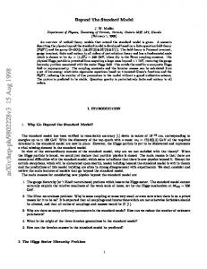
2.2.6 On the Cross Sections e+ e− → W + W − A very interesting example on how the Standard Model is able to improve the unitarity behavior of the cross sections is provided by the e+ e− → W + W − processes, which is presented in Fig. 5.
The first two diagrams are the t–channel neutrino exchange, similar to the contribution of Fig. 1, and the s–channel photon exchange. Both of them are present in any theory containing charged intermediate vector boson. However, the Standard Model introduces two new contributions: the neutral current contribution (Z exchange) and the Higgs boson exchange (H). The leading p–wave divergence of the neutrino diagram, which is proportional to s, is analogous to the one found in the reaction ν ν¯ → W + W − . However, in this case it is exactly canceled by the sum of the contributions of the photon (A) and the Z. This delicate canceling is a direct consequence of the gauge structure of the theory [96].
53
e-
W-
e-
neutrino W+
e+
W-
e-
A
neutrino
Z W+
e+ photon
e-
W-
W+
e+ Z boson
WH W+
e+ H boson
Fig. 5: Feynman diagram for the reaction e+ e− → W + W − . √ However, the s–wave scattering amplitude is proportional to (mf s) and, therefore, is also divergent at high energies. This remaining divergence is canceled by the Higgs exchange diagram. Therefore, the existence of a scalar boson, that gives rise to a s–wave contribution and couples proportionally to the fermion mass, is an essential ingredient of the theory. In Quigg’s words [1], “If the Higgs boson did not exist, we should have to invent something very much like it.”
54
2.3
Introducing the Quarks
In order to introduce the strong interacting particles in the Standard Model we shall first examine what happens with the hadronic neutral current when the Cabibbo angle (1.7) is taken into account. We can write the hadronic neutral current in terms of the quarks u and d′ , JµH (0) = u¯γµ (1 − γ5 )u + d¯′ γµ (1 − γ5 )d′ ¯ µ (1 − γ5 )d + sin2 θC s¯γµ (1 − γ5 )s = u¯γµ (1 − γ5 )u + cos2 θC dγ � � ¯ µ (1 − γ5 )s + s¯γµ (1 − γ5 )d . + cos θC sin θC dγ
We should notice that the last term generates flavor changing neutral currents (FCNC), i.e. transitions like d + s¯ ↔ d¯ + s, with the same strength of the usual weak interaction. However, the observed FCNC processes are extremely small. For instance, the branching ratio of charged kaons decaying via charged current is, � + + BR Ku¯ → µ+ ν ≃ 63.5% , s → W while process involving FCNC are very small [32]: � + + BR Ku¯ ¯ ≃ 4.2 × 10⁻¹⁰ , s → πud¯ν ν � L + − BR Kd¯ → µ µ ≃ 7.2 × 10⁻⁹ . s
In 1970, Glashow, Iliopoulos, and Maiani proposed the GIM mechanism [72]. They consider a fourth quark flavor, the charm (c), already introduced by Bjorken and Glashow in 1963. This extra quark completes the symmetry between quarks (u, d, c, and s) and leptons (νe , e, νµ , and µ) and suggests the introduction of the weak doublets � � � � u u = , LU ≡ cos θC d + sin θC s L d′ L � � � � c c . (2.39) = LC ≡ − sin θC d + cos θC s L s′ L and the right–handed quark singlets, RU ,
RD , 55
RS ,
RC .
(2.40)
Notice that now all particles, i.e. the T3 = ±1/2 fields, have also the right components to enable a mass term for them. In order to introduce the quarks in the Standard Model, we should start, just like in the leptonic case (2.10), from the free massless Dirac Lagrangian for the quarks, Lquarks = ¯LU i 6 ∂ LU + ¯LC i 6 ∂ LC ¯ U i 6 ∂ RU + · · · + R ¯ C i 6 ∂ RC . +R
(2.41)
We should now introduce the gauge bosons interaction via the covariant derivatives (2.11) with the quark hypercharges determined by the Gell-Mann–Nishijima relation (2.8), in such a way that the up–type quark charge is +2/3 and the down–type −1/3, YL = Q
1 , 3
YR = U
4 , 3
2 YR = − . D 3
(2.42)
Therefore, the charged weak couplings quark–gauge bosons, is given by, g (±) Lquarks = √ [¯ uγ µ (1 − γ5 )d′ + c¯γ µ (1 − γ5 )s′ ] Wµ+ + h.c. . 2 2
(2.43)
On the other hand, the neutral current receives a new contribution proportional to c¯γµ (1 − γ5 )c + s¯′ γµ (1 − γ5 )s′ and becomes diagonal in the quarks flavors, since the inconvenient terms of JµH (0) cancels out, avoiding the phenomenological problem with the FCNC. For instance, for the process K L → µ+ µ− , the GIM mechanism introduces a new box contribution containing the c–quark that cancels most of the u–box contribution and gives a result in agreement with experiment [97]. Finally, the neutral current interaction of the quarks become, X g (0) ψ¯q γ µ (gVq − gAq γ5 )ψq Zµ , (2.44) Lquarks = − 2cW ψ =u,··· ,c q
with the vector and axial couplings for the quarks given by (2.23) and (2.24), for i = q. 56
2.3.1 On Anomaly Cancellation In field theory, some loop corrections can violate a classical local conservation law, derived from gauge invariance via Noether’s theorem The so–called anomaly is a disaster since it breaks Ward–Takahashi identities and invalidate the proofs of renormalizability. The vanishing of the anomalies is so important that have been used as a guide for constructing realistic theories. Let us consider a generic theory with Lagrangian � ¯ γ µ T+a R + L ¯ γ µ T−a L Vµa , Lint = −g R
where T±a are the generators in the right (+) and left (−) representation of the matter fields, and Vµa are the gauge bosons. This theory will be anomaly free if abc Aabc = Aabc + − A− = 0 ,
where Aabc ± is given by the following trace of generators � a b c� Aabc ≡ Tr {T± , T± }T± . ±
In a V − A gauge theory like the Standard Model, the only possible anomalies come from V V A triangle loops, i.e. loops with two vectors and one axial vertex and are proportional to: X � � � � Y SU(2)2 U(1) : Tr {τ a , τ b }Y = Tr {τ a , τ b } Tr [Y ] ∝ doub.
3
U(1)
:
X � � Tr Y 3 ∝ Y3 . f erm.
Remembering the value of the hypercharge of the leptons (2.13) and quarks (2.42), we can write for the SU(2)2 U(1) case, � � �� X 1 abc A ∝− Y = − −1 + 3 =0, 3 doub.
57
and for the U(1)3 case, Aabc ∝
X
f erm
Y+3 − Y−3
(
"� � � �3 #) 3 4 −2 = (−2)3 + 3 + 3 3 ( "� � � �3 #) 3 1 1 =0. + − (−1)3 + (−1)3 + 3 3 3
where the 3 colors of the quarks were taken into account. This shows that the Standard Model is free from anomalies if the fermions appears in complete multiplets, with the general structure: � � � � �� νe u , eR , , u R , dR , e L d L that should be repeated always respecting this same structure: �� � � � � νµ c , µR , , cR , sR , µ L s L The discovery of the τ lepton in 1975 [77], and of a fifth quark flavor, the b [78], two years later, were the evidence for a third fermion generation, � � � � �� t ντ , tR , bR . , τR , b L τ L The existence of complete generations, with no missing partner, is essential for the vanishing of anomalies. This was a compelling theoretical argument in favor of the existence of a top quark before its discovery in 1995 [87, 88].
2.3.2 The Quark Masses In order to generate mass for both the up (Ui = u, c, and t) and down (Di = d, s, and b) quarks, we need a Y = −1 Higgs doublet. Defining the conjugate doublet Higgs as, � 0∗ � φ ∗ ˜ = i σ2 Φ = , (2.45) Φ −φ− 58
we can write the Yukawa Lagrangian for three generations of quarks as, Lqyuk
3 h � � X �i U ¯ † D ¯ † ˜ =− Gij RUi Φ Lj + Gij RDi Φ Lj + h.c. .
(2.46)
i,j=1
˜ doublets, we obtain From the vacuum expectation values of Φ and Φ the mass terms for the up ′ u U ′ ′ ′ ′ c + h.c. , (u , c , t )R M t′ L
and down quarks
(d′ , s′ , b′ )R MD
d′ s′ + h.c. , b′ L
U (D)
with the non–diagonal matrices Mij
√ U (D) = (v/ 2) Gij .
The weak eigenstates (q ′ ) are linear superposition of the mass eigenstates (q) given by the unitary transformations: ′ ′ d u d u ′ c′ s s c = DL,R , = UL,R , ′ ′ b b t t L,R L,R L,R L,R where U(D)L,R are unitary matrices to preserve the form of the kinetic terms of the quarks (2.41). These matrices diagonalize the mass matrices, i.e., mu 0 0 UR−1 MU UL = 0 mc 0 0 0 mt md 0 0 −1 DR MD DL = 0 ms 0 . 0 0 mb 59
The (V − A) charged weak current (2.43), for three generations, will be proportional to ′ d d (u′, c′ , t′ )L γµ s′ = (u, c, t)L (UL† DL ) γµ s , b′ L b L
with the generation mixing of the mass eigenstates (q) described by: V ≡ (UL† DL ) .
On the other hand, for the neutral current of the quarks (2.44), now becomes, ′ u u (u′ , c′ , t′ )L γµ c′ = (u, c, t)L (UL† UL ) γµ c . t′ L t L We can notice that there is no mixing in the neutral sector (FCNC) since the matrix UL is unitary: UL† UL = 1. The quark mixing, by convention, is that is with T3q = −1/2, ′ d s′ = V b′ L
restricted to the down quarks, d s . b L
V is the Cabibbo–Kobayashi–Maskawa matrix [61, 74], that can be parametrized as V = R1 (θ23 )R2 (θ13 , δ13 )R3 (θ12 ) , where Ri (θjk ) are rotation matrices around the axis i, the angle θjk describes the mixing of the generations j and k and δ13 is a phase. We should notice that, for three generations, it is not always possible to choose the V matrix to be real, that is δ13 = 0, and therefore the weak interaction can violate CP and T † . †
The violation of CP can also occur in the interaction of scalar bosons, when we have two or more scalar doublets. For a review see Ref. [98].
60
The Cabibbo–Kobayashi–Maskawa matrix can be written as c12 c13 s12 c13 s13 e−iδ13 s23 c13 , V = −s12 c23 − c12 s23 s13 eiδ13 c12 c23 − s12 s23 s13 eiδ13 iδ13 iδ13 s12 s23 − c12 c23 s13 e −c12 s23 − s12 c23 s13 e c23 c13
where sij (cij ) ≡ sin(cos)θi j. Notice that, in the limit of θ23 = θ13 → 0, we associate θ12 → θC , the Cabibbo angle (1.7), and c12 s12 0 V → −s12 c12 0 . 0 0 1 Using unitarity constraints and assuming only three generations the experimental value for the elements of the matrix V , with 90% of C.L., can be extract from weak quark decays and from deep inelastic neutrino scattering [32], 0.9742 − 0.9757 0.219 − 0226 0.002 − 0.005 V = 0.219 − 0.225 0.9734 − 09749 0.037 − 0.043 . 0.004 − 0.014 0.035 − 0.043 0.9990 − 0.9993
2.4
The Standard Model Lagrangian
We end this chapter giving a birds’ eye view of the Standard Model, putting all terms together and writing the whole Lagrangian in a schematic way. Gauge–boson + Scalar The gauge–boson (2.9) and the scalar (2.29) Lagrangians give rise to the free Lagrangian for the photon, W , Z, and the Higgs boson. Besides that, they generate triple and quartic couplings among the vector
61
bosons and also couplings involving the Higgs boson: Lgauge + Lscalar = 1 1 + − µν − Fµν F µν − Wµν W 4 2 1 Zµν Z µν + MZ2 Zµ Z µ + − 4 + W +W − A + W +W − Z
(2.47) 2 + MW Wµ+ W − µ
1 1 ∂µ H∂ µ H − MH2 H 2 2 2
+
W + W − AA + W + W − ZZ + W + W − AZ + W + W − W + W −
+
HHH + HHHH
+
W + W − H + W + W − HH + ZZH + ZZHH .
The vector–boson self–couplings that appear in (2.47) are strictly constrained by the SU(2)L ⊗ U(1)Y gauge invariance and any small deviation from the Standard Model predictions would destroy, for instance, the precise cancellation of the high–energy behavior between the various diagrams, giving rise to an anomalous growth of the cross section with energy. Therefore, the careful study of the vector–boson self–interactions is a important test of the Standard Model (see M. E. Pol, these Proceedings). Leptons + Yukawa The leptonic (2.14) and the Yukawa (2.36) Lagrangians are responsible for the lepton free Lagrangian and for the couplings with the gauge bosons: photon (QED interaction), W (charged weak current) and Z (neutral weak current). The mass terms are generated by the Yukawa interaction which also gives rise to the coupling of the massive lepton with the Higgs boson: Lleptons + Lℓyuk = X ¯ 6 ∂ − mℓ )ℓ + ℓ(i
ℓ=e,µ,τ
(2.48) X
νℓ =νe ,νµ ,ντ
ν¯ℓ (i 6 ∂)νℓ
+
ℓ¯ℓ A + ν¯ℓ ℓ W + + ℓ¯νℓ W − + ℓ¯ℓ Z + ν¯ℓ νℓ Z
+
ℓ¯ℓ H . 62
Even if the neutrinos have mass, as seems to suggest the recent experimental results [99, 100], their Dirac mass terms could be incorporated in the framework of the Standard Model without any difficulty. The procedure would be similar to the one that lead to the quark mass terms, that is, introducing a right–handed component of the neutrino and a Yukawa coupling with the conjugate Higgs doublet (2.45). One may notice, however, than being electrically neutral neutrinos may also have a Majorana mass which violates lepton number. The simultaneous existence of both type of mass terms, Dirac and Majorana, can be used to explain the smallness of the neutrino mass as compared to the charged leptons via the so called see-saw mechanism [101]. Quarks + Yukawa The quark Lagrangian (2.41) and the corresponding Yukawa interaction (2.46) give rise to the free Dirac term and to the electromagnetic and weak interaction of the quarks. A quark–Higgs coupling is also generated, Lquarks + LqYuk = X q¯(i 6 ∂ − mq )q
(2.49)
q=u,··· ,t
+
q¯ q A
+
u¯ d′ W + + d¯′ u W − + q¯ q Z
+
q¯ q H .
Besides the propagators and couplings presented above, in a general Rξ gauge, we should also take into account the contribution of the Goldstone bosons and of the ghosts. The Faddeev–Popov ghosts [70] are important to cancel the contribution of the unphysical (timelike and longitudinal) degrees of freedom of the gauge bosons. A practical guide to derive the Feynman rules for the vertex and propagators can be found, for instance, in Ref. [2], where the complete set of rules for the Standard Model is presented.
63
Chapter 3 Beyond the Trees 3.1
Radiative Corrections to the Standard Model
It was shown that the Standard Model is a renormalizable field theory. This means that when we go beyond the tree level (Born approximation) we are still able to make definite predictions for observables. The general procedure to evaluate these quantities at the quantum level is to collect and evaluate all the loop diagrams up to a certain level. Many of these contributions are ultraviolet divergent and a convenient regularization method (e.g. dimensional regularization) should be used to isolate the divergent parts. These divergences are absorbed in the bare couplings and masses of the theory. Assuming a renormalization condition (e.g. on–shell or MS scheme), we can evaluate all the counterterms. After all these ingredients are put together we are able to obtain finite results for S–matrix elements that can be translated in, for instance, cross sections and decay widths. The predictions of the Standard Model for several observables are obtained and can be compared with the experimental results for these quantities enabling the theory to be falsified (in the Popperian sense). The subject of renormalization is very cumbersome and deserves a whole course by itself. Here we want to give just the minimum necessary tools to enable the reader to appreciate the astonishing agreement 64
of the Standard Model, even at the quantum level, with the recent experimental results. Very good accounts of the electroweak radiative corrections can be found elsewhere [102, 103, 104]. Let us start considering the Standard Model Lagrangian which is given by the sum of the contributions (2.47), (2.48), and (2.49). The LSM is a function of coupling constants g and g ′ and of the vacuum expectation value of the Higgs field, v. The observables can be determined in terms of these parameters and any possible dependence on other quantities like MH or mt appears just through radiative corrections. Therefore, we need three precisely known observables in order to determine the basic input parameters of the model. A natural choice will be the most well measured quantities, like, e.g.: • The electromagnetic fine structure constant that can be extracted, for instance, from the electron ge − 2 or from the quantum Hall effect, α(0) = 1/137.0359895(61) ; • The Fermi constant measured from the muon lifetime, GF (µ) = 1.16639(1) × 10−5 GeV−2 ; • The Z boson mass that was obtained by LEP at the Z pole, MZ = 91.1867(21) GeV . These input parameters can be written, at tree level, in terms of just g, g ′ and v as g 2 s2W , 4π 1 , = √ 2v 2 g2v2 = . 4c2W
α0 (0) = GF 0 MZ20
65
(3.1)
where the subscript 0 indicates that these relations are valid at tree level, and s2W ≡
g′ 2 , g2 + g′ 2
and c2W ≡
g2 , g2 + g′ 2
depend only on g and g ′ :
3.1.1 One Loop Calculations Let us write the vacuum polarization amplitude (self–energy) for vector bosons (a, b = γ, W, Z) as 2 µν Πµν Πab (q 2 ) + (q µ q ν terms) . ab (q ) ≡ g
The terms proportional to q µ q ν can be dropped since these amplitudes should be plugged in conserved fermion currents, and from the Dirac equation, they will give rise to terms that goes with the external fermion mass that can be neglected in the usual experimental situation. We can summarize the relevant quantities for the loop corrections of the Standard Model [103]: • The vector and axial form factors of the Z 0 coupling, at q 2 = MZ2 , which include both the vertex and the fermion self–energy radiative corrections. From (2.21) we can write g µ VZf = −i ψ¯f γ µ (gVf − gAf γ5 )ψf , f¯ 2 cos θW where (2.23) and (2.24) now are given by � √ � f gVf = ρ T3 − 2 κf Qf sin2 θW , √ f ρ T3 . gAf =
(3.2)
which define the relative strength of the neutral and charged currents, ρ, and the coefficient of the sin2 θW , κf . Notice that at tree level, ρ = κf = 1. 66
• Correction to µ–decay amplitude at q 2 = 0, which includes the box (B), vertex (V ) and the fermion self–energy corrections � �� � M(µ) = −i δG(B,V ) ψ¯e γ µ (1 − γ5 )ψνe ψ¯νµ γ µ (1 − γ5 )ψµ . We can write the corrections to the input parameters as, α = α0 + δα , MZ2 = MZ20 + δMZ2 , GF = GF0 + δGF ,
(3.3)
where, in terms of the vacuum polarization amplitude, and δG(B,V ) the corrections become δα sW ΠγZ (0) = −Πγγ (0) − 2 , α cW MZ2 δMZ2 ΠZZ (MZ2 ) = − , (3.4) MZ2 MZ2 δGF ΠW W (0) δG(B,V ) = . + 2 GF MW GF Correction to the Derived Observables From the corrections to the input parameters we can estimate the radiative corrections to the derived observables. Let us write the tree level input variables α0 , GF0 , and MZ0 as I0i . When we compute the radiative correction to the input parameters I0i , we have I0i −→ I i (I0i ) = I0i + δI i (I0i ) .
The relation for the renormalized input variables, I i , can be inverted to write I0i = I0i (I i ).
The same holds true for any derived observable (O) or any S–matrix element, that is, O[I0i (I i )] = O0 (I0i ) + δO(I0i ) = O0 (I i − δI i ) + δO(I i − δI i ) X ∂O0 = O0 (I i ) − δI i + δO(I i ) i ∂I i ≡ O0 (I i ) + ∆O(I i ) . 67
(3.5)
At one loop it is enough to renormalize just the input variables I i . However, at two loops it is necessary also to renormalize all other parameters that intervene at one loop level like mt and MH . As an example, let us compute the radiative correction to the W boson mass. At tree level MW is given by [see (2.31)] 2 MW = c2W0 MZ20 . 0
Writing c2W in terms of the input variables, we have � � �� � � �� 4πα πα 2 2 cW = (1 − sW ) = 1 − = 1− √ . g2 2GF MZ2 c2W Solving for c2W , we get ( " �1/2 #) � 4πα 1 2 MZ2 . 1+ 1− √ (I i ) = MW 0 2 2GF MZ2 Taking into account the derivatives, 2 ∂MW 0 ∂α 2 ∂MW 0 ∂GF 2 ∂MW 0 ∂MZ2
s2W c2W MZ2 , s2W − c2W α s2 c2 MZ2 = − 2 W W2 , sW − cW G F c4 = − 2 W 2 . sW − cW =
We obtain from (3.5) the MW correction 2 MW
= =
2 MW (I i ) 0
c2W MZ2
−
−
2 X ∂MW
0
∂I i � 2
i 2 cW MZ 2 sW − c2W
2 δI i + δMW (I i )
s2W
δα δGF δMZ2 − s2W − c2W α GF MZ2
with 2 2 δMW = −ΠW W (MW ).
68
�
2 + δMW ,
3.2
The Z boson Physics
3.2.1 Introduction The most important experimental tests of the Standard Model in this decade was performed at the Z pole. The four LEP Collaborations (Aleph, Delphi, L3, and Opal)[105] and the SLAC SLD Collaboration [106] studied the reaction, e+ e− → Z 0 → f f¯ . The main purpose of these experiments was to test the Standard Model at the level of its quantum corrections and also to try to obtain some hint on the top quark mass and on the Higgs boson.
Fig. 6: The Z profile measured by the L3 Collab. [107] At CERN, after scanning the Z resonance (see Fig. 6), data were collected at the Z peak, and around 17 millions of Z’s were produced and studied. 69
The shape of the resonance is characterised by the cross section for the fermion pair (f f¯) production at the Z peak, σf0f¯ =
12π Γe Γf , MZ2 Γ2Z
where the position of the peak gives the value MZ = 91186.7 ± 2.1 MeV, the full width at half maximum (FWHM) represents the Z width, ΓZ = 2493.9 ± 2.4 MeV, and the height of the peak gives the value of the total cross section for f f¯ production, σf0f¯. For the analysis of the Z physics it is necessary to choose the input parameters at the appropriate scale, MZ . The relative uncertainty of the input parameters are: Parameter
Value
Uncertainty
mt [108]
174.3 ± 5.1 GeV
2.9 %
αs (MZ2 ) [105] α−1 (MZ2 ) [109, 110] MZ [105] GF (µ) [32]
0.119 ± 0.002
128.878 ± 0.090
91186.7 ± 2.1 MeV
(1.16639 ± 0.00001) × 10−5 GeV−2
1.7 % 0.07 % 0.0023 % 0.00086 %
Table I: Relative uncertainty of the input parameters. For the Higgs boson mass we just have available a lower bound of MH > 95.2 GeV at 95% of C.L. [111]. Notice that, in spite of the very precise measurement of the electromagnetic structure constant at low energy, which has a relative uncertainty of just 0.0000045 %, its value at MZ is much less precise. This uncertainty arises from the contribution of light quarks to the vacuum polarization. The evolution of α is given by α(MZ2 ) =
α(0) , 1 − ∆α
70
(3.6)
where ∆α = ∆αlep + ∆αhad + ∆αtop . The top quark contribution is proportional to 1/m2t ∼ 10−5 . The contributions from leptons (ℓ) [110] and light quarks (q) [109] are: ∆αlep = 0.031498 , ∆αhad = −(0.02804 ± 0.00065) .
(3.7)
where the error in ∆αlep is negligible. Therefore, the loss of precision comes from ∆αhad due to non–perturbative QCD effects that are large at low energies and to the imprecision in the light quark masses. Other important pure QED corrections are the initial and final state photon radiation. The initial state radiation is taken into account by convoluting the cross section with the radiator function H(k), σ(s) =
Z
kmax
0
dk H(k)σ0 [s(1 − k)] ,
where kmax represents a cut in the maximum radiated energy. The radiator function takes into account virtual and real photon emissions and includes soft photon resummation [112]. The final state radiation is included by multiplying the bare cross sections and widths by the QED correction factor, � � 3αQ2f 1+ ≃ (1 + 0.002 Q2f ) . 4π where Qf is the fermion charge.
3.2.2 The Standard Model Parameters We present in the following sections the Standard Model predictions for some observables. We compare these predictions with the values measured by the CERN LEP and at the SLAC SLD Collaborations, and stress the very impressive agreement between them. 71
Z Partial Widths The Z width into a fermion pair, at tree level, is given in the Standard Model by, i GF M 3 h Γ(Z → f f¯) = C √ Z (gAf )2 + (gVf )2 , 6 2π
(3.8)
where C refers to the fermion color, i.e., � 1 , for leptons , C= 3 [1 + αs (MZ )/π + 1.409αs2 (MZ )/π 2 + · · · ] , for quarks . where the QCD corrections were included for quarks. At loop level we should consider the modifications to gVf and gAf (3.2) and the appropriate QED corrections discussed in the last section. The value of the partial width for the different fermion flavors are f f¯ Pair
Partial Width 167.25 MeV 84.01 MeV 300.30 MeV 383.10 MeV 376.00 MeV
ν ν¯ e e u¯ u dd¯ b¯b
+ −
Table II: Z → f f¯ partial widths. The experimental results for the partial widths are [105], Γℓ ≡ Γhad ≡ ΓZ ≡ Γinv ≡
Γ(Z → ℓ+ ℓ− ) = 83.90 ± 0.10 MeV , Γ(Z → hadrons) = 1742.3 ± 2.3 MeV , Γ(Z → all) = 2493.9 ± 2.4 MeV , ΓZ − 3 Γℓ − Γhad = 500.1 ± 1.9 GeV ,
where we assume three leptonic channels (e+ e− , µ+ µ− , and τ + τ − ), and Γinv is the invisible Z width. 72
Number of Neutrino Species We can extract information on the number of light neutrino species by supposing that they are responsible for the invisible width, i.e. Γinv = Nν Γν . The LEP data [105] gives the ratio of the invisible and leptonic Z partial widths, Γinv /Γℓ = 5.961 ± 0.023. On the other hand, Standard Model predicts the (Γν /Γℓ )SM = 1.991 ± 0.001, where the error is associated to the variation of mt and MH . In the ratio of these two expressions, Γℓ cancels out and yields the number of neutrino species, Nν = 2.994 ± 0.011 , where Nν represents the total number of neutrino flavors that are accessible kinematically to the Z, that is Mν < MZ /2. This result indicates that, if the observed pattern of the first three generations is assumed, then we have only these families of fermions in nature. Radiative Corrections Beyond QED An important question to be asked when comparing the Standard Model predictions with experimental data is if the effect of pure weak radiative correction could indeed be measured. This question can be answered by looking, for instance, at the plot of sin2 θeff × Γℓ (Fig. 7), where Γℓ is given by (3.8) and, � � 1 gVℓ 2 sin θeff ≡ 1 − ℓ = 0.23157 ± 0.00018 . 4 gA The point at the lower–left corner shows the prediction when only the QED (photon vacuum polarization) correction is included and the respective variation for α(MZ2 ) varying by one standard deviation. The Standard Model prediction, with the full (QED + weak) radiative correction, is represented by the band that reflects the dependence on the Higgs (95 GeV < MH < 1000 GeV) and on the top mass (169.2 GeV < mt < 179.4 GeV). We notice that the presence of genuine electroweak correction is quite evident.
73
mt= 174.3 ± 5.1 GeV mH= 95...1000 GeV
0.233 0.2325
sin2θeff
lept
mH
0.232
0.2315 0.231
∆α
mt
Preliminary
83.6
68% CL
83.8
84
84.2
Γl [MeV] Fig. 7: LEP + SLD measurements of sin2 θeff and Γℓ , compared to the Standard Model prediction [113].
Another important evidence for pure electroweak correction comes from the radiative correction ∆rW to the relation between MW and GF , � 2 � 2 MW πα(MZ2 ) MW √ , (3.9) = 1− 2 MZ MZ2 2GF MZ2 (1 − ∆rW ) where α(MZ2 ) is given by (3.6), and therefore, the effect of the running of α was subtracted in the definition of ∆rW . Taking into account the value measured at LEP and Tevatron, MW = 80.394 ± 0.042 GeV, we have [104]: (∆r)exp W = −0.02507 ± 0.00259. Thus, the correction representing only the electroweak contribution, not associated with the running of α, is ∼ 10 σ different from zero.
74
gVℓ , gAℓ , and the Lepton Universality The partial Z width in the different lepton flavors is able to provide a very important information on the universality of the electroweak interactions. The values of gVℓ and gAℓ can be plotted for ℓ = e, µ and τ .
-0.031
Preliminary
-0.035
gVl
mH
-0.039
mt Al (SLD) +−
ll + − ee + − µµ + − ττ
-0.043
-0.503
68% CL
-0.502
-0.501
-0.5
gAl Fig. 8: 68% C.L. contours in the gVℓ × gAℓ plane. The solid line is a fit assuming lepton universality. The band corresponds to the SLD result from ALR (3.12) measurements [113]. The result present in Fig. 8 shows that the measurements of gVℓ × gAℓ are consistent with the hypothesis that the electroweak interaction is universal and yields gVℓ = −0.03703 ± 0.00068 , 75
gAℓ = −0.50105 ± 0.00030 .
Notice that the value of gAℓ disagrees with the Born prediction of −0.5 (2.24) by 3.5 σ. However they are in very good agreement with the Standard Model values [32]: (gVℓ )SM = −0.0397 ± 0.0003 and (gAℓ )SM = −0.5064 ± 0.0001. This is another important evidence of the weak radiative corrections. Asymmetries Since parity violation comes from the difference between the right and left couplings of the Z 0 to fermions, it is convenient to define the combination of the vector and axial couplings of the fermions as Af =
2gVf gAf (gVf )2 + (gAf )2
.
(3.10)
The events e+ e− → f + f − can be characterized by the momentum direction of the emitted fermion. We say that the final state fermion (f − ) travels forward (F ) or backward (B) with respect to the electron (e− ) beam. Therefore, we can define the forward–backward asymmetry by AF B ≡
σF − σB , σF + σB
and at the Z pole, this asymmetry is given by 3 A0F,Bf = Ae Af . 4
(3.11)
The measurement of A0F ,Bf for charged leptons, and c and b quarks give us information only on the product of Ae and Af . On the other hand, the measurement of the τ lepton polarization is able to determine the values of Ae and Aτ separately. The longitudinal τ polarization is defined as Pτ ≡
σR − σL , σR + σL
76
where σR(L) is the cross section for tau–lepton pair production of a right (left) handed τ − . At the Z pole, Pτ can be written in terms of scattering (e− , τ − ) angle θ as, Pτ = −
Aτ (1 + cos2 θ) + 2Ae cos θ . 1 + cos2 θ + 2Ae Aτ cos θ
This yields [105] Ae = 0.1479 ± 0.0051 , Aτ = 0.1431 ± 0.0045 , which are in agreement with the lepton universality (Aℓ = 0.1469 ± 0.0027). They are also in agreement with the Standard Model prediction: ASM = 0.1475 ± 0.0013. ℓ
This result can be used to extract information on the heavy quark couplings: Ac = 0.646 ± 0.043 and Ab = 0.899 ± 0.025, which should be compared with the Standard Model values of ASM = 0.6679 ± 0.0006 and c SM Ab = 0.9348 ± 0.0001.
Another interesting asymmetry that can be measured by SLD is the left–right cross section asymmetry, ALR =
σL − σR , σL + σR
(3.12)
where σL(R) is the cross section for (left–) right–handed incident electron with the positron kept unpolarized. Since, at the Z pole, ALR = Ae , we can get the best measurement of the electron couplings: Ae = 0.1510 ± 0.0025 (see Fig. 8). Higgs Mass Sensitivity In order to give an idea of the sensitivity of the different electroweak observables to the Higgs boson mass, we compare in Fig. 9 the experimental values with the the Standard Model theoretical predictions, as a function of MH . The vertical band represents the experimental measurement with the respective error. The theoretical prediction includes the errors in α(MZ2 ), from ∆αhad (3.7), αs (MZ2 ), and mt (see Table I). 77
3
3
mH [GeV]
10
mH [GeV]
10
10
2
10
3
2.49
10
2
10
3
2.5
0.015
0.02
AFB0,l
mH [GeV]
mH [GeV]
ΓZ [GeV]
10
2
10
3
10 41.4
41.6
0.095
σ0 h [nb]
0.1
0.105
AFB0,b
3
mH [GeV]
10
mH [GeV]
2
10
2
10 20.7
20.8
2
0.06
0.07
Rl 3
3
mH [GeV]
10
mH [GeV]
10
0.08
AFB0,c
10
2
10
3
0.14
10
2
10
3
0.16
0.232
sin Θ
lepteff
0.234
from
mH [GeV]
mH [GeV]
0.23 2
Aτ
10
2
10
3
10 0.14
0.16
2
80.25
80.5
mW [GeV]
Ae
Measurement
mH [GeV]
∆α(5) had= 0.02804 ± 0.00065
10
αs= 0.119 ± 0.002 mt= 174.3 ± 5.1 GeV 2
0.14
0.16
Al (SLD)
Fig. 9: LEP measurements compared with the Standard Model predictions, as a function of MH [113]. 78
In this figure σh0 is the hadronic cross section at the Z pole, Rℓ ≡ (Γhad /Γℓ ). A0F,Bf is defined in (3.11) and Af in (3.10). < QF B > is the average charge, which is related to the forward–backward asymmetries by < QF B >=
X
δq AqF B
q
Γqq¯ , Γhadr
where δq is the average charge difference between the q and q¯ hemispheres. For the sake of comparison Ae , extracted by SLD from ALR (3.12), is also shown. We can see from Fig. 9 that dependence on the Higgs mass varying in the range 95 GeV < MH < 1000 GeV is quite mild for all the observables, since the Higgs effect enters only via log(MH2 /MZ2 ) factors.
6
theory uncertainty ∆α(5) had = 0.02804±0.00065 0.02784±0.00026
∆χ2
4
2
0
Excluded 10
Preliminary
10
2
mH [GeV]
10
3
Fig. 10: ∆χ2 ≡ χ2 − χ2min as a function of MH [105, 113]. 79
However we can extract information on MH from the global fit including all data on the different observables. In Fig. 10 we show the plot of ∆χ2 ≡ χ2 − χ2min versus MH . The left vertical band represents > the excluded region due to the direct search for the Higgs (MH ∼ 95 GeV). The band represents an estimate of the theoretical error due to missing higher order corrections. The global fit results in MH = 91+64 −41 GeV.
mZ [GeV] ΓZ [GeV] 0
σhadr [nb]
Measurement
Pull
91.1871 ± 0.0021
.08
2.4944 ± 0.0024
-.56
41.544 ± 0.037
1.75
20.768 ± 0.024
1.16
Afb
0.01701 ± 0.00095
.80
Ae
0.1483 ± 0.0051
.21
Aτ
0.1425 ± 0.0044
-1.07
Re 0,e
2 lept
sin θeff
0.2321 ± 0.0010
.60
mW [GeV]
80.350 ± 0.056
-.62
Rb
0.21642 ± 0.00073
Rc
0.1674 ± 0.0038
-1.27
0,b
0.0988 ± 0.0020
-2.20
Afb
0,c
0.0692 ± 0.0037
-1.23
Ab
0.911 ± 0.025
-.95
Ac
0.630 ± 0.026
-1.46
Afb
2 lept
sin θeff 2
.81
0.23099 ± 0.00026 -1.95
sin θW
0.2255 ± 0.0021
1.13
mW [GeV]
80.448 ± 0.062
1.02
mt [GeV] (5)
∆αhad(mZ)
Pull -3 -2 -1 0 1 2 3
174.3 ± 5.1
.22
0.02804 ± 0.00065
-.05
-3 -2 -1 0 1 2 3
Fig. 11: Comparison of the precision electroweak measurements with the Standard Model predictions [113]. As a final comparison, we present in Fig. 11 a list of several electroweak observables. The experimental values are compared with the Standard Model theoretical predictions. The Pull ≡ (Omeas − Ofit )/σmeas , represents the number of standard deviations that separate the central values. This results show an impressive agreement with the Standard Model expectations. 80
Chapter 4 The Higgs Boson Physics
4.1
Introduction
The procedure of generating vector boson masses in a gauge invariant way requires the introduction of a complex doublet of scalar fields (2.25) which corresponds to four degrees of freedom. Three out of these are “eaten” by the gauge bosons, W + , W − , and Z 0 , and become their longitudinal degree of freedom. Therefore, it remains in the physical spectrum of the theory the combination (φ0 + φ¯0 ) √ =H +v , 2 where v is given by (2.27), and H is the physical Higgs boson field. The Higgs boson mass (2.34) can be written as √ !1/2 p √ √ 2 λ. MH = −2µ2 = 2λ v = GF
(4.1)
Both Higgs potential parameters, µ2 and λ, are a priori unknown — just their ratio is fixed by the low energy data [see (2.17) and (2.31)]. Therefore the Standard Model does not provide any direct information on the Higgs boson mass. 81
The discovery of this particle is one of the challenges of the high– energy colliders. This is the most important missing piece of the Standard Model and its experimental verification could furnish very important information on the spontaneous breaking of the electroweak symmetry and on the mechanism for generating fermion masses. The phenomenology of the Standard Model Higgs boson is covered in great detail in reference [114]. Recent review articles include Ref. [115], [116], [117], [118]. We intend to emphasize here the most relevant properties of Higgs particle and make a brief summary of the prospects for its search in the near future.
4.2
Higgs Boson Properties
The Higgs Couplings The Higgs boson couples to all particles that get mass (∝ v) through the spontaneous symmetry breaking of SU(2)L ⊗ U(1)Y . We collect in Table III the intensity of the coupling to the different particles from (2.30), (2.33), (2.36), and (2.46), Coupling
Intensity
Hf f¯ HW + W − HZ 0 Z 0 HHW + W − HHZ 0 Z 0 HHH HHHH
Mf /v 2 2MW /v 2 MZ /v 2 MW /v 2 MZ2 /2v 2 MH2 /2v MH2 /8v 2
Table III: The Higgs coupling to different particles. From the results of Table III it becomes evident that the Higgs couples proportionally to the particle masses. Therefore we can establish two general principles that should guide the search of the Higgs boson: 82
(i) it will be produced in association with heavy particles; (ii) it will decay into the heaviest particles that are accessible kinematically. Besides the couplings presented in Table III, the Higgs can also couple to γγ [119], Zγ [120, 121] and also to gluons [122, 123], at one loop level. The neutral and weak interacting Higgs boson can interact with photons through loops of charged particles that share the weak and electromagnetic interactions: leptons, quarks and W boson. In the same way the Higgs couples indirectly with the gluons via loops of (weak and strong interacting) quarks. Bounds on the Higgs Boson Mass Since the Higgs boson mass is not predicted by the model we should rely on some experimental and theoretical bounds to guide our future searches. The most stringent lower bound was recently established by the LEP Collaborations [111] and read MH > 95.2 GeV . at 95% C.L.. It is also possible to obtain a theoretical lower bound on the Higgs boson mass based on the stability of the Higgs potential when quantum corrections to the classical potential (2.26) are taken into account [124]. Requiring that the standard electroweak minimum is stable (i.e. the vacuum is an absolute minimum) up to the Planck scale, Λ = 1019 GeV, the following bound can be established [125]: � � αs − 0.12 MH (in GeV) > 133 + 1.92(mt − 175) − 4.28 . 0.006 The behavior of MH as a function of the scale Λ is given in the lower curve of Fig. 13, for mt = 175 GeV and αs = 0.118. We see from this figure that, if a Higgs boson is discovered with MH ≃ 100 GeV, it would mean that the electroweak vacuum is instable at Λ ∼ 105 GeV ∗ . ∗
Reversing the argument, since we live in a stable vacuum, this means that the Standard Model must break down at this same scale.
83
There are also some theoretical upper bounds on the Higgs boson mass. A bound can be obtained by requiring that unitarity is not violated in the scattering of vector bosons [126]. Let us take as an example the W W scattering represented in Fig. 12.
W
W
W A
Z W
W
W
W
W
W
W
W
W
W
W
W
W
Z
W
W H
W
W
A W
W
W
W H W
W
W
W
Fig. 12: Feynman contributions to W + W − → W + W − . We should notice that if we exclude the Higgs boson contribution by taking MH → ∞, we expect that the remaining amplitudes would eventually violate unitarity, since the theory is not renormalisable without the Higgs. Therefore, it is natural to expect that the Higgs mass should play an important rˆole in high energy behaviour of the scattering amplitudes of longitudinally polarized vector bosons. This is what happened for instance in the reaction e+ e− → W + W − discussed in section 2.2. A convenient way to estimate amplitudes involving longitudinal gauge bosons is through the use of the Goldstone Boson Equivalence The84
orem [126, 127]. This theorem states that at high energies, the amplitude M for emission or absorption of a longitudinally polarized gauge boson is equal to the amplitude for emission or absorption of the corresponding Goldstone boson, up to terms that fall like 1/E 2 , i.e., � 2 M(WL± , ZL0 ) = M(ω ± , z 0 ) + O MW,Z /E 2 . (4.2)
We can use an effective Lagrangian approach to describe the Goldstone boson interactions. Starting from the Higgs doublet in terms of ω ± and z 0 , � � √ 1 i 2ω + Φ= √ , 0 2 v + H − iz we can write the Higgs potential as V (Φ† Φ) = µ2 Φ† Φ + λ(Φ† Φ)2 1 2 2 g MH2 2 = MH H + H(H 2 + 2ω + ω − + z 0 ) 2 4 MW 2 2 g MH 2 (H 2 + 2ω + ω − + z 0 )2 . + 2 32 MW Therefore, with the aid of (4.2), the amplitude for WL+ WL− → WL+ WL− is obtained as, M(WL+ WL− → WL+ WL− ) ≃ M(ω + ω − → ω + ω − ) � � g 2 MH2 MH2 MH2 = −i 2+ + . 2 4 MW s − MH2 t − MH2 and, at high energies, we have: M(ω + ω − → ω + ω − ) ≃ −i
√ g 2 MH2 2GF MH2 . = −i 2 2 2 MW
Therefore, for s-wave, unitarity requires A0 =
2GF 1 |M(ω +ω − → ω + ω − )| = √ MH2 < 1 . 16π 8π 2 85
When this result is combined with the other possible channels (z 0 z 0 , < z 0 h, hh) it leads to the requirement that λ ∼ 8π/3 or, translated in terms of the Higgs mass, √ !1/2 8π 2 < MH ∼ ≃ 1 TeV . 3GF Another way of imposing a bound on the Higgs mass is provided by the analysis of the triviality of the Higgs potential [124]. The renormalization group equation, at one loop, for the quartic coupling λ is � 1 dλ = 12λ2 + (terms involving g, g ′, Yukawa) , 2 dt 16π
where t = log(Q2 /µ2 ). Therefore, for a pure φ4 potential, i.e., when the gauge and Yukawa couplings are neglected, we have the solution � 2� 1 1 3 Q − = 2 log . λ(µ) λ(Q) 4π µ2 Since the stability of the Higgs potential requires that λ(Q) ≥ 0, we can write λ(µ) ≤
4π 2 , 3 log(Q2 /µ2 )
(4.3)
and, for large values of Q2 , we can see that λ(µ) → 0 and the theory becomes trivial, that is, not interacting. The relation (4.3), can be written as � � 4π 2 2 2 . Q ≤ µ exp 3λ(µ) This result gives rise to a bound in the Higgs boson mass when we consider the scale µ2 = MH2 and take into account (4.1), � 2 2� 8π v 2 2 Q ≤ MH exp . 3MH2 Therefore, there is a maximum scale Q2 = Λ2 , for a given Higgs boson mass, up to where the Standard Model theory should be valid. 86
Fig. 13: Perturbative and stability bound on MH as a function of the scale Λ, from Ref. [125].
In Fig. 13, we present the stability bound (lower curve) and the triviality bound (upper curve) on the Higgs boson mass as a function of the scale Λ. If we expect that the Standard Model is valid up to a given scale — let us say ΛGUT ∼ 1016 GeV [128] — a bound on the Higgs mass < < should lie between both curves, in this case 140 GeV ∼ MH ∼ 180 GeV.
4.3
Production and Decay Modes
4.3.1 The Decay Modes of the Higgs Boson The possible decay modes of the Higgs boson are essentially determined by the value of its mass. In Fig. 14 we present the Higgs branching ratio for different MH . When the Higgs boson mass lies in the range 95 GeV < MH < 130 GeV, the Higgs is quite narrow ΓH < 10 MeV and the main branching 87
1
_ bb
WW
BR(H) ZZ 10
-1
+ −
ττ _ cc
tt-
gg 10
-2
γγ Zγ 10
-3
50
100
200 MH [GeV]
500
1000
Fig. 14: The branching ratios of the Higgs boson as a function of its mass from Ref. [117].
ratios come from the heaviest fermions that are accessible kinematically: BR(H → b¯b) ∼ 90% , BR(H → c¯ c) ≃ BR(H → τ + τ − ) ∼ 5% . For MH ≃ 120 GeV the gluon–gluon channel is important giving a contribution of ∼ 5% of the width. For a heavier Higgs, i.e. MH > 130 GeV, the vector boson channels H → V V ∗ , with V = W , Z, are dominant, BR(H → W + W − ) ∼ 65% , BR(H → Z 0 Z 0 ) ∼ 35% . For MH ≃ 500 GeV the top quark pair production contributes with ∼ 20% of the width. Note that the BR(H → γγ) is always small O(10−3 ). However, we can think of some alternative models that give rise to larger Hγγ couplings (for a review see [129] and references therein). For large values of MH the Higgs becomes a very wide resonance: ΓH ∼ [MH (in TeV)]3 /2. 88
4.3.2 Production Mechanisms at Colliders Electron–Positron Colliders The Higgs boson can be produced in electron–positron collisions via the Bjorken mechanism [130] or vector boson fusion [131], (i) Bjorken: (ii) WW Fusion: (iii) ZZ Fusion:
e+ + e− → Z → Z H ,
e+ + e− → ν ν¯(W W ) → ν ν¯ H ,
e+ + e− → e+ e− (ZZ) → e+ e− H .
√ At LEPI and II, where s ≃ MZ or 2 MW the Higgs production is dominated by the Bjorken mechanism and they were able to rule out from very small Higgs masses up to 95.2 GeV [111]. Maybe, when the whole analysis is complete, they will be able to rule out up to MH ∼ 106 GeV. + − At the √ future e e accelerators, like the Next Linear Collider [132], where s = 500 GeV, the production of a Higgs with 100 < MH < 200 GeV will be dominated by the W W fusion, since its cross section behaves like σ ∝ log(s/MH2 ) and therefore dominates at high energies. We can expect around 2000 events per year for an integrated luminosity of L ≃ 50 fb−1 , and the Next Linear Collider should be able to explore up to MH ∼ 350 GeV.
Hadron Colliders At proton–(anti)proton collisions the Higgs boson can be produced via the gluon fusion mechanism [122, 123], through the vector boson fusion and in association with a W ± or a Z 0 ,
(i) Gluon fusion:
p¯ p → gg → H ,
(ii) VV Fusion: (iii) Association with V: 89
p¯ p→VV →H ,
p¯ p → q q¯′ → V H .
√ At the Fermilab Tevatron [133], with s = 1.8 (2) TeV, the Higgs is better produced in association with vector boson and they look for the V H(→ b¯b) signature. After the improvement in the luminosity at TEV33 they will need L ∼ 10 fb−1 to explore up to MH ∼ 100 GeV with 5 σ. √ At the CERN Large Hadron Collider [134], that will operate with s = 14 TeV, the dominant production mechanism is through the gluon fusion and the best signature will be H → ZZ → 4 ℓ± for MH > 130 GeV. For MH < 130 GeV they should rely on the small BR(H → γγ) ∼ 10−3 . We expect that the LHC can explore up to MH ∼ 700 GeV with an integrated luminosity of L ∼ 100 fb−1 . Once the Higgs boson is discovered it is important to establish with precision several of its properties like mass, spin, parity and width. The next step would be to search for processes involving multiple Higgs production, like V V → HH or gg → HH, which could give some information on the Higgs self–coupling.
90
Chapter 5 Closing Remarks In the last 30 years, we have witnessed the striking success of a gauge theory for the electroweak interactions. The Standard Model made some new and crucial predictions. The existence of a weak neutral current and of intermediate vector bosons, with definite relation between their masses, were confirmed by the experiments. Recently, a set of very precise tests were performed by Tevatron, LEP and SLC colliders that were able to reach an accuracy of 0.1% or even better, in the measurement of the electroweak parameters. This guarantees that even the quantum structure of the model was successfully confronted with the experimental data. It was verified that the W and Z couplings to leptons and quarks have exactly the same values anticipated by the Standard Model. We already have some strong hints that the triple–gauge–boson couplings respect the structure prescribed by the SU(2)L ⊗ U(1)Y gauge symmetry. The Higgs boson, remnant of the spontaneous symmetry breaking, has not yet been discovered. However, important information, extracted from the global fitting of data taking into account the loop effects of the Higgs, assures that this particle is just around the corner. The Higgs mass should be less than ∼ 260 GeV at 95% C.L., in full agreement with the theoretical upper bounds for the Higgs mass. These remarkable achievements let just a small room for the new physics beyond the Standard Model. Nevertheless, we still have some
91
conceptual difficulties like the hierarchy problem, that may indicate that the explanation provided by the Standard Model should not be the end of the story. A series of alternative theories — technicolour, grand unified theory, supersymmetric extensions, superstrings, extra dimension theories, etc — have been proposed, but they all suffer from lack of an experimental spark. Nevertheless, the physics beyond the Standard Model is also beyond the scope of these lectures . . .
Acknowledgments We are grateful to M. C. Gonzalez–Garcia and T. L. Lungov for the critical reading of the manuscript. This work was supported by Conselho Nacional de Desenvolvimento Cient´ıfico e Tecnol´ogico (CNPq), by ˜ de Amparo a` Pesquisa do Estado de Sao ˜ Paulo (FAPESP), Fundac¸ao ´ by Programa de Apoio a Nucleos de Excelˆencia (PRONEX), and by ˜ para o Desenvolvimento da Universidade Estadual Paulista Fundac¸ao (FUNDUNESP).
92
Bibliography [1] C. Quigg, Gauge Theories of the Strong, Weak, and Electromagnetc Interactions (Addison–Wesley Pub. Co., Menlo Park, 1983). [2] T. P. Cheng and L.-F. Li, Gauge Theory of Elementary Particle Physics (Claredon Press, Oxford, 1984). [3] The partial Z width in the different lepton flavors is able to provide a very important information on the universality of the electroweak interactions. The values of gVℓ and F. Halzen and A. D. Martin, Quarks and Leptons: An Introductory Course on Modern Particle Physics (John Wiley & Sons, New York, 1984). [4] I. J. R. Aitchison and A. J. G. Hey, Gauge Theories in Particle Physics : A Practical Introduction (Adam Hilger, Bristol, 1990). [5] P. Renton, Electroweak Interactions: An Introduction to the Physics of Quarks and Leptons (Cambridge University Press, Cambridge, 1990). [6] E. Golowich J. F. Donoghue and B. R. Holstein, Dynamics of the Standard Model (Cambridge University Press, Cambridge, 1992). [7] E. Predazzi E. Leader, An Introduction to Gauge Theories and Modern Particle Physics (Cambridge University Press, Cambridge, 1996). [8] E. S. Abers and B. W. Lee, Phys. Rep. 9, 1 (1973). [9] M. Levine J. E. Kim, P. Langacker and H. H. Williams, Rev. Mod. Phys. 53, 211 (1981). 93
[10] M. A. B. Beg and A. Sirlin, Phys. Rep. 88, 1 (1982). [11] M. S. Chanowitz, Ann. Rev. Nucl. Part. Sci. 38, 323 (1988). [12] R. N. Cahn and G. Goldhaber, The Experimental Foundations of Particle Physics (Cambridge Univ. Press, Cambridge, 1989). [13] V. V. Ezhela et al., Particle Physics: One Hundred Years of Discoveries (American Institute of Physics, New York, 1996). [14] J. Schwinger (editor), Selected Papers on Quantum Electrodynamics (Dover Pub., Inc., New York, 1981). [15] C. H. Lai (editor), Selected Papers on Gauge Theory of Weak and Electromagnetic Interactions (World Scientific, Singapore, 1981). [16] H. Becquerel, Compt. Ren. 122, 501 (1896), (Five papers were published in the same issue. See also pages 559, 689, 762, and 1086). [17] J. Chadwick, Verhandl Dtsch. Phys. Ges. 16, 383 (1914). [18] C. D. Ellis and W. A. Wooster, Proc. Roy. Soc. A117, 109 (1927). [19] P. A. M. Dirac, Proc. Roy. Soc. A114, 243 (1927); idem, A114, 710 (1927). [20] W. Pauli, Open Letter to Radioactive Persons, 1930, for an English translation see: Physics Today 31, 27 (1978). [21] J. R. Oppenheimer, Phys. Rev. 35, 461 (1930). [22] W. Pauli, in Septi`eme Conseil de Physique, Solvay (Gauthier– Villars, Paris, 1934), p. 324. [23] E. Fermi, Z. Phys. 88, 161 (1934); idem, Nuovo Cim. 11, 1 (1934). [24] G. Gamow and E. Teller, Phys. Rev. 49, 895 (1936). [25] F. Bloch and A. Nordsieck, Phys. Rev. 52, 54 (1937). [26] E. J. Williams and G. E. Roberts, Nature 145, 102 (1940).
94
[27] S. Tomonaga, Bull. I. P. C. R. (Riken Iho) 22, 545 (1943), for the English translation see Prog. Theor. Phys. 1, 27 (1946). [28] B. Pontecorvo, Phys. Rev. 72, 246 (1947). [29] H. A. Bethe, Phys. Rev. 72, 339 (1947). [30] P. Kusch and H. M. Foley, Phys. Rev. 72, 1256 (1947). [31] J. Schwinger, Phys. Rev. 73, 416 (1948). [32] C. Caso et al., The European Physical Journal 1 (1998). [33] R. P. Feynman, Phys. Rev. 74, 1430 (1948); idem, 76, 769 (1949). [34] J. Schwinger, Phys. Rev. 74, 1439 (1948); idem, 75, 651 (1949). [35] T. Tati and S. Tomonaga, Prog. Theor. Phys. 3, 391 (1948); see also: Z. Koba, T. Tati and S. Tomonaga, Prog. Theor. Phys. 2, 101 and 198 (1947). [36] F.J. Dyson, Phys. Rev. 75, 486 (1949). [37] J. Tiomno and J. A. Wheeler, Rev. Mod. Phys. 21, 144 (1949). [38] T. D. Lee, M. N. Rosenbluth, and C. N. Yang, Phys. Rev. 75, 905 (1949). [39] J. C. Ward, Phys. Rev. 78, 182 (1950). [40] C. N. Yang and R. L. Mills, Phys. Rev. 96, 191 (1954). [41] L. W. Alvarez and S. Goldhaber, Nuovo Cim. 2, 344 (1955). [42] R. W. Birge et al., Phys. Rev. 100, 430 (1955). [43] T. D. Lee and C. N. Yang, Phys. Rev. 104, 254 (1956). [44] C. S. Wu et al., Phys. Rev. 105, 1413 (1957). [45] R. L. Garwin, L. M. Lederman, and M. Weinrich, Phys. Rev. 105, 1415 (1957). [46] J. I. Friedman and V. L. Teledgi, Phys. Rev. 105, 1681 (1957). 95
[47] H. Frauenfelder et al., Phys. Rev. 106, 386 (1957). [48] A. Salam, Nuovo Cim. 5, 299 (1957). [49] T. D. Lee and C. N. Yang, Phys. Rev. 105, 1671 (1957). [50] L. D. Landau, Zh. Eksp. Teor. Fiz. 32, 407 (1957); see also JETP 5, 337 (1957). [51] J. Schwinger, Ann. Phys. 2, 407 (1957). [52] T. D. Lee and C. N. Yang, Phys. Rev. 108, 1611 (1957). [53] R. P. Feynman and M. Gell-Mann, Phys. Rev. 109, 193 (1958). [54] R. E. Marshak and E. C. G. Sudarshan, Phys. Rev. 109, 1860 (1958). [55] J. J. Sakurai, Nuovo Cim. 7, 649 (1958). [56] J. Leite Lopes, Nucl. Phys. 8, 234 (1958). [57] M. Goldhaber, L. Grodzins, and A. W. Sunyar, Phys. Rev. 109, 1015 (1958). [58] J. Goldstone, Nuovo Cim. 19, 154 (1961); see also: Y. Nambu, Phys. Rev. Lett. 4, 380 (1962). [59] A. Salam and J. C. Ward, Nuovo Cim. 19, 165 (1961). [60] S. L. Glashow, Nucl. Phys. 22, 579 (1961). [61] N. Cabibbo, Phys. Rev. Lett. 10, 531 (1963). [62] S. L. Glashow J. D. Bjorken, Phys. Lett. 11, 255 (1964). [63] P. W. Higgs, Phys. Lett. 12, 132 (1964). [64] F. Englert and R. Brout, Phys. Rev. Lett. 13, 321 (1964). [65] G. S. Guralnik, C. R. Hagen, and T. W. B. Kibble, Phys. Rev. Lett. 13, 585 (1964).
96
[66] J. H. Christenson, J. W. Cronin, V. L. Fitch, and R. Turlay, Phys. Rev. Lett. 13, 138 (1964). [67] A. Salam and J. C. Ward, Phys. Lett. 13, 168 (1964). [68] T. W. B. Kibble, Phys. Rev. 155, 1554 (1967). [69] S. Weinberg, Phys. Rev. Lett. 19, 1264 (1967). [70] L. D. Faddeev and V. N. Popov, Phys. Lett. B 25, 29 (1967). [71] A. Salam, in “Elementary Particle Theory”, The Nobel Symposium no 8, edited by N. Svartholm (Almqvist and Wiksell, Stock¯ holm, 1968), p. 367. [72] S. L. Glashow, J. Iliopoulos, and L. Maiani, Phys. Rev. D 2, 1285 (1970). [73] G. ’t Hooft, Nucl. Phys. B33, 173 (1971); idem, B35, 167 (1971). [74] M. Kobayashi and T. Maskawa, Prog. Theor. Phys. 49, 652 (1973). [75] F. J. Hasert et al., Phys. Lett. B 46, 121 (1973); idem, B 46, 138 (1973). [76] A. Benvenuti et al., Phys. Rev. Lett. 32, 800 (1974). [77] M. L. Perl et al., Phys. Rev. Lett. 35, 1489 (1975). [78] S. W. Herb et al., Phys. Rev. Lett. 39, 252 (1977). [79] G. Arnison et al. (UA1 Collab.), Phys. Lett. B 122, 103 (1983). [80] M. Banner et al. (UA2 Collab.), Phys. Lett. B 122, 476 (1983). [81] G. Arnison et al. (UA1 Collab.), Phys. Lett. B 126, 398 (1983). [82] P. Bagnaia et al. (UA2 Collab.), Phys. Lett. B 129, 130 (1983). [83] R. S. Van Dyck, P. B. Schwinberg, and H. G. Dehmelt, Phys. Rev. D 34, 722 (1986). [84] H. Albrecht et al. (ARGUS Collab.), Phys. Lett. B 192, 245 (1987). 97
[85] G. S. Abrams et al. (MARK–II Collab.), Phys. Rev. Lett. 63, 2173 (1989). [86] LEP Collaborations: ALEPH, DELPHI, L3 and OPAL, Phys. Lett. B 276, 247 (1992). [87] F. Abe et al. (CDF Collab.), Phys. Rev. Lett. 74, 2626 (1995). [88] S. Abachi et al. (DØ Collab.), Phys. Rev. Lett. 74, 2632 (1995). [89] D. J. Gross and F. Wilczek, Phys. Rev. Lett. 30, 1343 (1973). [90] H. D. Politzer, Phys. Rev. Lett. 30, 1346 (1973). [91] W. Heisenberg, Z. Phys. 77, 1 (1932). [92] R. Utiyama, Phys. Rev. 101, 1597 (1956). [93] S. Weinberg, The Quantum Theory of Fields (Cambridge University Press, Cambridge, 1996), vol. II, pp. 164–167. [94] S. A. Bludman, Nuovo Cim. 9, 433 (1958). [95] B. W. Lee K. Fujikawa and Sanda, Phys. Rev. D 6, 2923 (1972). [96] C. H. Llwellyn Smith, Phys. Lett. B 46, 233 (1973). [97] M. K. Gaillard and B. W. Lee, Phys. Rev. D 10, 897 (1974). [98] B. Winstein and L. Wolfenstein, Rev. Mod. Phys. 65, 1113 (1993). [99] Y. Suzuki, talk given at the XIX International Symposium on Lepton and Photon Interactions at High Energies Stanford University (1999). [100] T. Mann, talk given at the XIX International Symposium on Lepton and Photon Interactions at High Energies Stanford University (1999). [101] R. Slansky M. Gell-Mann, P. Ramond, in Supergravity, , edited by P. van Nieuwenhuizen and D. Z. Freedman (North Holland Publ. Co., Amsterdan, 1979), pp. Print–80–0576 (CERN); see also, R. Mohapatra and G. Senjanovic, Phys. Rev. Lett. 44, 912 (1980). 98
[102] W. Hollik, in Particle and Fields, Proceedings of the VII J. A. ´ Swieca Summer School, edited by O. J. P. Eboli and V. O. Rivelles (World Scientific, Singapore, 1994), p. 169. [103] R. Barbieri, in 1994 European School of High Energy Physics, Proceedings of the 1994 European School of High Energy Physics, edited by N. Ellis and M. B. Gavela (CERN, Geneva, 1995), p. 43. [104] A. Sirlin, talk given at the XIX International Symposium on Lepton and Photon Interactions at High Energies Stanford University (1999), hep-ph/9912227. [105] The LEP Collaborations ALEPH, DELPHI, L3, OPAL, the LEP Electroweak Working Group and the SLD Heavy Flavour and Electroweak Groups, Technical Report No. CERN–EP/99–15 (unpublished). [106] S. Willocq (for the SLD Collaboration), in The strong interaction, from hadrons to partons, Proceedings of the 24th Annual SLAC Summer Institute on Particle Physics: The Strong Interaction, From Hadrons to Protons, edited by L. Dixon J. Chan, L. DePorcel (Springfield, NTIS, 1997), p. 405. [107] B. Adeva et al. (L3 Collab.), Phys. Lett. B 247, 473 (1990). [108] S. Kim (for the CDF and DØ Collaborations), Technical Report No. FERMILAB–Conf-99/262–E (unpublished). [109] S. Eidelmann and F. Jegerlehmer, Z. Phys. 585 (1995). [110] M. Steinhauser, Phys. Lett. B 429, 158 (1998). [111] ALEPH, DELPHI, L3, OPAL, and the LEP Working Group for Higgs Boson Searches, Technical Report No. ALEPH 99– 081 CONF 99-052, submitted to the International Europhysics Conference on High Energy Physics, Tampere, Finland (unpublished). [112] O. Nicrosini G. Montagna and F. Piccinini, Phys. Lett. B 406, 243 (1997). 99
[113] See also the LEP Electroweak Working Group Home Page, http://www.cern.ch/LEPEWWG/ (Summer 99 Plots). [114] G. Kane J. F. Gunion, H. E. Haber and S. Dawson, The Higgs Hunter’s Guide (Addison–Wesley Pub. Co., Menlo Park, 1990), and references therein. [115] B. A. Kniehl, Phys. Rep. 240, 211 (1994). [116] A. Djouadi, Int. J. Mod. Phys. A 10, 1 (1995). [117] M. Spira and P. Zerwas, in 36th International University School of Nuclear and Particle Physics: Computing Particle Properties (36 IUKT), Lecture Notes in Physics 512, edited by C. B. Land H. Gausterer (Springer, Berlin, 1998), p. 161. [118] C. Quigg, Acta Phys. Polon. B30, 2145 (1999). [119] M. K. Gaillard J. Ellis and D. V. Nanopoulos, Nucl. Phys. B 106, 292 (1976). [120] N. Fleishon R. N. Cahn, M. S. Chanowitz, Phys. Lett. B 82, 113 (1979). ˜ A. Barroso, J. Pulido, Nucl. Phys. B 267, 509 (1986). [121] J. C. Romao [122] M. E. Machacek D. V. Nanopoulos H. M. Georgi, S. L. Glashow, Phys. Rev. Lett. 40, 692 (1978). [123] S. F. Novaes, Phys. Rev. D 27, 2211 (1983). [124] M. Sher, Phys. Rep. 179, 273 (1989). [125] M. Quiros J. A. Casas, J. R. Espinosa, Phys. Lett. B 342, 171 (1995); see also M. Quiros, in Perspectives on Higgs Physics II, edited by G. L. Kane (World Scientific, Singapore, 1997), hepph/9703412. [126] H. B. Thacker B. W. Lee, C. Quigg, Phys. Rev. D 16, 1519 (1977). [127] M. Chanowitz and M. K. Gaillard, Nucl. Phys. B 261, 379 (1985).
100
[128] G. G. Ross, Grand Unified Theories (Addison–Wesley Pub. Co., Menlo Park, 1984), and references therein. [129] M. C. Gonzalez-Garcia, Int. J. Mod. Phys. A 14, 3121 (1999). [130] J. D. Bjorken, Proccedings of the Summer Institute on Particle Physics, Technical Report No. SLAC-198 (unpublished). [131] R. Cahn and S. Dawson, Phys. Lett. B 136, 196 (1984), [E: B 138, 464 (1984)]. [132] H. Murayama and M. E. Peskin, Ann. Rev. Nucl. Part. Sci. 46, 533 (1996), E. Accomando et al., Phys. Rep. 299, 1 (1998). [133] W. Marciano A. Stange and S. Willenbrock, Phys. Rev. D 49, 1354 (1994); idem, D 50, 4491 (1994). [134] D. Graudenz M. Spira, A. Djouadi and P. M. Zerwas, Nucl. Phys. B 453, 17 (1995).
101