colliding set, before executing actual primitive-level queries. Our ... 3 Preliminaries. Our algorithm evaluates self-intersections on 2-manifold triangle meshes ...
Star-Contours for Efficient Hierarchical Self-Collision Detection Sara C. Schvartzman
´ Alvaro G. P´erez URJC Madrid
Miguel A. Otaduy
Abstract Collision detection is a problem that has often been addressed efficiently with the use of hierarchical culling data structures. In the subproblem of self-collision detection for triangle meshes, however, such hierarchical data structures lose much of their power, because triangles adjacent to each other cannot be distinguished from actually colliding ones unless individually tested. Shape regularity of surface patches, described in terms of orientation and contour conditions, was proposed long ago as a culling criterion for hierarchical self-collision detection. However, to date, algorithms based on shape regularity had to trade conservativeness for efficiency, because there was no known algorithm for efficiently performing 2D contour self-intersection tests. In this paper, we introduce a star-contour criterion that is amenable to hierarchical computations. Together with a thorough analysis of the tree traversal process in hierarchical self-collision detection, it has led us to novel hierarchical data structures and algorithms for efficient yet conservative self-collision detection. We demonstrate the application of our algorithm to several example animations, and we show that it consistently outperforms other approaches.
1
Introduction
Highly deformable objects, such as cloth, threads, plants, flesh, or articulated objects, often suffer collisions against themselves. Detecting self-collision has long posed a challenge to computer animation, and it often becomes the bottleneck in simulations, in particular for cloth animation. We are interested in the acceleration of self-collision detection for triangle meshes. For inter-object collision detection between deformable bodies, hierarchical algorithms based on bounding volume hierarchies offer an attractive solution as long as the bodies do not suffer topology changes. They carry a moderate update cost, and their query cost smoothly adapts to the inherent complexity of the collision configuration. In self-collision detection, however, hierarchical algorithms based on bounding volumes suffer a particular problem: tests between triangles adjacent to each other cannot be culled away at high levels in the hierarchy, and even situations without actual collisions turn out to be computationally expensive. Volino and Magnenat-Thalmann [1994] introduced a hierarchical self-collision detection technique based on shape regularity, which does not suffer from difficulties induced by adjacency. Their work has been continued by many others, who have improved the efficiency of elementary tests [Provot 1997], incorporated continuous collision detection [Tang et al. 2008], optimized computations for
2D projection
2D projection
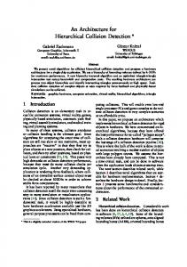
Figure 1: Examples of contours with and without selfintersections. In the bottom image, a surface patch in the knee of the cat self-intersects. This patch passes the orientation test, but its 2D-projected contour self-intersects. Our algorithm executes contour tests in a conservative yet efficient way. specific types of deformations [Schvartzman et al. 2009], designed parallelizable extensions [Baciu and Wong 2002], or extended it to subdivision surfaces [Grinspun and Schr¨oder 2001]. However, this line of work also suffers one important limitation: efficiency must be traded for conservativeness. One step in the original algorithm, known as the contour test, cannot guarantee a cost independent of the resolution of the triangle mesh, which is a requirement for strictly efficient hierarchical collision detection. In this paper, we present a hierarchical self-collision detection algorithm for triangle meshes that is both conservative and efficient. The algorithm misses no collisions (up to geometric degeneracies or rounding errors), and it fulfills the basic requirements for efficiency of hierarchical collision detection algorithms [Gottschalk 2000]. Our novel algorithm builds on the approach of Volino and Magnenat-Thalmann, and it uses the same underlying geometric criteria for culling away non-colliding surface patches, but it presents several important contributions in its data structures and algorithms. We also introduce a novel analysis of hierarchical selfcollision detection, which lays the grounds for our algorithmic improvements. Specifically, the main novelties in our work are: ∙ A novel contour test based on the star-shaped property of a polygon, amenable to hierarchical computations (Section 4). ∙ The analysis of the traversal process of hierarchical selfcollision detection, resulting in a novel tree data structure, the self-collision test tree. It simplifies the traversal algorithm and becomes the central data structure of our method (Section 5). ∙ A hierarchical data structure of patch contour segments for efficient execution of the star-contour test (Section 6). We have evaluated our algorithm on a variety of examples, including cloth animations, other thin shell simulations, character skinning, or meshes animated with finite element models. It outperforms spatial hashing by 2× to 6×, and AABB-trees by up to 4×.
2
Related Work
A number of different methods have been designed for the evaluation of self-collision detection on deformable models. One option is to use a spatial partitioning, as in the case of optimized spatial hashing [Teschner et al. 2003]. The main features of this method are that it does not rely on any preprocessing and it does not impose requirements on the characteristics of the triangle meshes to be tested, hence it has a very wide applicability. On the other hand, this method has a high offset cost as every primitive (or a bound) needs to be tested against several other primitives. Its performance is also rather sensitive to the variance in triangle size. Another approach to self-collision detection based on spatial partitioning is to use discrete Voronoi diagrams [Sud et al. 2006], which has the additional benefit of allowing for distance computations. Bounding volume hierarchies (BVHs), independently of the type of BV used (AABBs, OBBs, 𝑘-DOPs, spheres, etc.), rely on a series of properties in order to provide strictly efficient queries. For a triangle mesh with 𝑛 triangles, the branching factor of the tree must be 𝑂(1), the depth 𝑂(lg 𝑛) (these two conditions together imply size 𝑂(𝑛)), the cost to perform an elementary test on a BV 𝑂(1), and the cost to update the complete hierarchy 𝑂(𝑛) (in an amortized sense, it implies an 𝑂(1) cost per BV) [Gottschalk 2000]. When used with deformable objects, they are typically updated in a bottom-up fashion [Van den Bergen 1997]. However, these conditions do not guarantee efficiency in practice, as this depends on the collision configuration as well. Self-collision queries with BVHs are executed by starting a recursive query on the root BV against itself. Unfortunately, adjacent triangle pairs force many branches of the collision query to expand all the way to the leaves of the BVH. Mezger et al. [2003] applied BVHs to self-collision detection, using in particular inflated 𝑘-DOPs, but they added the shape regularity criterion [Volino and Magnenat-Thalmann 1994] to improve performance. One of the positive aspects of BVHs is that they can be used for interruptible collision detection, even with on-demand update of BVs [James and Pai 2004]. Visibility-based culling techniques [Govindaraju et al. 2003] return a set of potentially colliding triangles, and they require further processing in order to identify potentially colliding pairs. Their main asset is that they provide very high performance in practice, thanks to their parallelism and implementation on graphics hardware architectures. Govindaraju et al. [2005] later combined visibility-based culling and a chromatic decomposition of the triangle mesh, in order to radically improve the performance of self-collision detection using BVHs. Specifically, they proposed a first step based on an AABB-tree query for identifying potentially colliding pairs of triangles, and then additional steps based on visibility queries and chromatic decomposition that drastically reduced the potentially colliding set, before executing actual primitive-level queries. Our work is complementary to theirs, as our algorithm could replace and outperform the initial AABB-tree query, which is, incidentally, the bottleneck in their algorithm. As mentioned in the introduction, our work is closest to hierarchical self-collision detection based on shape regularity [Volino and Magnenat-Thalmann 1994]. This approach partitions hierarchically a triangle mesh into connected patches, and prunes away surface patches that fulfill two tests: (i) The orientation test searches for a direction that has a positive dot product with the normals of all triangles in the patch; and (ii) the contour test checks whether the contour of the patch projected along the aforementioned direction is intersection-free. The initial algorithm employed discrete normal cones for the orientation test, while Provot [1997] improved performance using actual cones. Baciu and Wong [2002] adopted many of the ideas into a parallel algorithm and implemented it on graphics hardware. More recently, Tang et al. [2008] have incorporated
Figure 2: Deflating horse benchmark, with 25K triangles and large self-colliding regions. Our algorithm outperforms AABBtrees by 1.8× at the beginning of the simulation, and it remains slightly faster when the complete mesh has degraded at the end. additional adjacency-related optimizations, as well as an extension of the original orientation and contour tests to the continuous collision detection setting. Grinspun et al. [2001] have applied it in the context of subdivision surfaces, and Schvartzman et al. [2009] to certain reduced deformations. Although the shape regularity approach is in theory an elegant one, the design of an efficient algorithm has posed important problems so far. The original implementation avoided the contour test, and pruned surface patches with a valid orientation test. As shown in Fig. 1, the decision of ignoring the contour test may introduce missed collisions. As noted by several researchers [Grinspun and Schr¨oder 2001; Tang et al. 2008], the contour test can itself be solved using bounding data structures. √Contours of patches high in the hierarchy are expected to have 𝑂( 𝑛) edges, hence a hierarchical contour test is not guaranteed to run in constant time. Moreover, the edge-hierarchy of every patch needs to be updated, with √ cost up to 𝑂( 𝑛), and it is not clear how to reuse edge-hierarchies of low levels when computing edge-hierarchies at high levels. We conclude that, to the best of our knowledge, there is no efficient algorithm for the contour test. Before describing the contributions of our work, let us anticipate that a large part of the novelty lies on the application of star-shaped polygon tests to the self-collision detection problem. Star-shaped polygon tests have also seen application in other problems, such as roadmap computation [Varadhan and Manocha 2005], or the art gallery problem [Avis and Toussaint 1981].
3
Preliminaries
Our algorithm evaluates self-intersections on 2-manifold triangle meshes, possibly with boundaries. For objects with multiple connected components, we simply handle each component separately. Semi-regular meshes are beneficial for the performance of the algorithm, as it depends on aspects such as the number of triangles adjacent to each triangle. Given a triangle mesh, we partition it to create a binary tree of connected patches. Each patch must itself constitute one connected component. Again, a good partitioning, formed by patches with smooth boundaries and semi-regular size per level, is beneficial for the performance of the algorithm. For each patch in the binary tree, we store a bounding volume and a normal cone. In our implementation, we have used AABBs and discrete normal cones (DNCs) with 14 directions [Volino and Magnenat-Thalmann 1994], respectively. The binary tree of bounding volumes constitutes a BVH.
In the following sections, we describe data structures and algorithms that allow for an efficient application of the star-contour test in hierarchical self-collision detection. Thanks to these data structures and algorithms, the contour test of a patch can be executed with cost 𝑂(1), regardless of the number of edges in the contour, provided that the given mesh and its hierarchical partitions have a bounded vertex valence.
5
Figure 3: General Vs. line-search star-shaped test. Top: a starshaped polygon showing its kernel (left), and the application of our line-search approach (right). 𝑡 and 𝑏 indicate, respectively, the lower bound of top edges (in blue) and the upper bound of bottom edges (in red). Bottom: an example polygon whose contour passes the interior-halfplanes test, but fails the ray-to-infinity test, which yields two intersections.
4
Star-Contour Test
We propose a star-shaped polygon test as a sufficient condition for determining whether the contour of a projected patch is free of intersections. A polygon is defined to be star-shaped if and only if there exists at least one point q such that, for all points p in the polygon, the line segment pq lies entirely inside the polygon [Lee and Preparata 1979]. Considering the contour of the polygon to be opaque, the complete polygon must be visible from point q. The set of points q that fulfill the condition form the kernel of the polygon. The definition of star-shapedness can be broken into two conditions (up to geometric degeneracies): (i) There must exist a point that lies on the interior half-planes defined by all the contour edges, and (ii) a ray-to-infinity from that point must intersect the contour once. The first condition can be formulated as a linear programming problem, with cost linear in the number of edges. The second condition can also be tested with a cost linear in the number of edges if no preprocessing is performed. These two conditions, but in particular the linear program, do not appear amenable for a hierarchical algorithm, which is a key condition for the application of star-shapedness as an efficient yet conservative contour selfintersection test. In order to design efficient tests, we restrict the search for a kernel point to a line, thus turning the linear program into a line-search problem. Under no preprocessing, the line-search also bears a linear cost, but we will demonstrate that it is well-suited for hierarchical computations.
Self-Collision Test Tree (SCTT)
The traversal process of a hierarchical collision detection algorithm can be represented as a tree, the Bounding Volume Test Tree (BVTT) [Gottschalk 2000], where a node contains two patches of the BVH that are tested for collision. We define as the Self-Collision Test Tree (SCTT) the subtree of the BVTT whose nodes contain two adjacent patches. Nodes of the SCTT represent self-collision tests for pairs of adjacent patches. Fig. 4a shows an example mesh and its hierarchical partitioning, Fig. 4b shows its associated BVH, and Fig. 4c shows its SCTT. Formally, we define the root of the SCTT as the node containing the two children of the root of the BVH, (𝐵𝑉 𝐻𝑟𝑜𝑜𝑡.𝑙𝑒𝑓 𝑡, 𝐵𝑉 𝐻𝑟𝑜𝑜𝑡.𝑟𝑖𝑔ℎ𝑡). Then, we define the rest of the nodes recursively in the following manner. For a node (𝐴, 𝐵), we define its children nodes as {(𝐴.𝑐ℎ𝑖𝑙𝑑, 𝐵.𝑐ℎ𝑖𝑙𝑑)}, if 𝐴.𝑐ℎ𝑖𝑙𝑑 and 𝐵.𝑐ℎ𝑖𝑙𝑑 are adjacent. Moreover, if 𝐴 and 𝐵 have the same parent in the BVH, i.e., 𝐴.𝑝𝑎𝑟𝑒𝑛𝑡 = 𝐵.𝑝𝑎𝑟𝑒𝑛𝑡, we also define as children nodes (𝐴.𝑙𝑒𝑓 𝑡, 𝐴.𝑟𝑖𝑔ℎ𝑡) and (𝐵.𝑙𝑒𝑓 𝑡, 𝐵.𝑟𝑖𝑔ℎ𝑡). Pairs of children that are not adjacent constitute nodes of the BVTT, but not the SCTT, and they are shown in red in Fig. 4c. For unbalanced BVHs, the construction of the SCTT can be eased by the definition of the Extended BVH (xBVH). As shown in Fig. 4b, the xBVH is formed by replicating leaf nodes of the BVH down to the level of the deepest leaf. The xBVH also plays a key role in the construction of contour segments, explained in Section 6. Unlike earlier approaches to hierarchical self-collision detection, we explicitly create the SCTT as a preprocessing step based on patch adjacency information and the traversal process of a selfcollision query. Hierarchical self-collision detection can then be easily formulated as the top-down traversal of the SCTT. When a node of the SCTT is visited, its associated patch is first tested for a valid orientation. If this test succeeds, its contour is tested for self-intersection. We formulate this test in a conservative manner using our star-contour criterion. In the next section, we describe the hierarchical data structures for efficient formulation of the starcontour test. In the special case where two adjacent BVH nodes share only one vertex, our star-contour test would always fail on their combined patch. Their SCTT node requires simple though special handling, which is described in the Appendix.
Given the contour of a polygon, let us separate its edges into top and bottom ones, according to their orientation w.r.t. a search line 𝐿. For every edge 𝑒, we consider its associated ray 𝑟(𝑒). Then, the polygon is guaranteed to be star-shaped if the following two conditions hold: (i) the lowest intersection 𝑡 of top edge rays with 𝐿 is higher than the highest intersection 𝑏 of bottom edge rays with 𝐿, i.e., 𝑡 > 𝑏; and (ii) the search line 𝐿 intersects only one top edge. These conditions constitute the basis for our star-contour test. Fig. 3 shows two examples of the application of our star-contour test.
Another positive result of preprocessing the SCTT is that, unlike earlier approaches, we do not need to query for patch adjacency at runtime. The storage requirements of the SCTT are low for semiregular meshes. If every patch is adjacent to 𝑂(1) patches at the same level, then the SCTT has 𝑂(𝑛) nodes, where 𝑛 is the number of triangles in the mesh.
In practice, we choose as search lines the middle vertical and horizontal lines of the AABB enclosing the polygon. We choose these lines based on the heuristic that the kernel, if it exists, is likely to lie somewhere in the center of the polygon. Using both search lines instead of just one produced up to a 10% speed-up on our benchmarks, while adding a 3𝑟𝑑 line turned more expensive.
As presented in Section 4, our algorithm executes a star-shape test as a sufficient condition for pruning patch contours that do not selfintersect. The algorithm outlined in Section 4 is based on the intersection of edge rays with a search line. In this section, we present an efficient version of the algorithm that exploits a hierarchical representation of contour segments. We start by describing this hier-
6 Contour Segments
$ " )*$$!
+"#,!
"#$$! %&'(!
%&'(!
!"
#
% "
! %
!"#$"#-"#,#
."#-"#/"#!#
" & " ! # ! &
# &
1"#)"#*"# -"#/"#0!
!"#$"#-"#/!
!"#$"#%"## 0"#-"#'"#(# )"#*"%"#!# &"#'"#(!
(a) Mesh Partitioning
#&%+&,-! "(./(%+0!
(b) xBVH
(c) SCTT
(d) CSF
Figure 4: Examples of the data structures used in our algorithm: (a) Partitioning of a triangle mesh at 4 levels, showing contour segments. (b) BVH and xBVH (with xBVH nodes shown in dotted red lines). (c) SCTT, with each node showing the two patches involved, and the list of contour segments that surround them. The node (𝐷, 𝐶) is a node of the BVTT, but not the SCTT, because 𝐷 and 𝐶 are not adjacent. (d) Contour Segment Forest (CSF) for the same example. archical representation, followed by the actual star-shape test using contour segments. Then, we describe the efficient update of the hierarchical contour representation. And we conclude by introducing a novel method for bounding bundles of rays in 2D, which is a key building block of our actual star-shape test.
6.1
Contour Segment Forest (CSF)
A node of the xBVH is present in several SCTT nodes, specifically, in as many as its number of adjacent xBVH nodes at the same level, as shown in Fig. 4c. Various parts of the contour of the xBVH node may then be visited in several star-shape tests. Following this observation, and in the context of the star-shape test, instead of testing every contour edge individually against the search line, we have designed a conservative test that utilizes bounds of contour segments, and tests for intersection between those bounds and the search line. We define as a contour segment a continuous set of edges shared by two adjacent xBVH nodes of the same level. Contour segments of one xBVH node can be constructed by merging contour segments of its children nodes. Therefore, we define the Contour Segment Forest (CSF) as the hierarchical data structure whose nodes correspond to individual contour segments, and the children of a segment 𝑎 correspond to other segments that are merged to produce 𝑎. This hierarchical data structure is a forest, not a tree, because the contour segments defining the boundary between two sibling xBVH nodes simply ‘disappear’ from the xBVH when the nodes merge. The same contour segment may exist at various consecutive levels of the xBVH, as long as it suffers no modifications during the merging of xBVH nodes. Since the star-shape test defined in Section 4 separates the edges into top and bottom ones, for practical reasons and ease of implementation, we define the contour segments as oriented segments. Then, the continuous boundary between two adjacent xBVH nodes defines two different contour segments. Fig. 4a shows an example mesh with the contour segments at all levels of the BVH, Fig. 4c indicates the lists of contour segments that surround each SCTT node for the same mesh, and Fig. 4d shows the full CSF. At runtime, our algorithm stores the CSF and the list of contour segments surrounding each SCTT node. The CSF is an efficient data structure from the point of view of both complexity and storage. Assuming semi-regular meshes with balanced partitioning and smooth patch boundaries, each xBVH node is adjacent to 𝑂(1) other nodes. Therefore, the size of the CSF is
𝑂(𝑛), being 𝑛 the number of triangles in the surface. In our implementation, we construct the CSF in a bottom-up manner. First, we define the oriented half-edges of the triangle mesh as the contour segments for the leaves of the xBVH, and we set them as the leaf nodes of the CSF. Then, we construct the CSF by analyzing the merging operations of xBVH nodes, creating a new contour segment whenever old ones can be merged, and setting child-parent relationships accordingly. We store temporarily for each xBVH node a list of its contour segments, and these lists are later used for creating the list of contour segments of each SCTT node.
6.2
Star-Contour Test with Contour Segments
Based on the star-contour test outlined in Section 4, we propose here a modified version that is amenable to efficient implementation using the CSF. Instead of testing individually each contour edge or edge ray of an SCTT node 𝐴 against a search line 𝐿, the efficient algorithm tests bounds of contour segments. As a result, the expected cost of a star-contour test for an SCTT node becomes 𝑂(1). For each contour segment 𝑠, we define a top subsegment 𝑠.𝑡𝑜𝑝 and a bottom subsegment 𝑠.𝑏𝑜𝑡𝑡𝑜𝑚. The top subsegment is formed by the top edges in the segment, and similarly for the bottom subsegment. Fig. 5-left shows an example patch contour, its contour segments, and top and bottom subsegments for one particular segment. For each subsegment, we store an interval that bounds its horizontal extent (assuming a vertical search line), as well as bounds for its edge rays. For top subsegments we compute lower bounds of edge rays, while for bottom subsegments we compute upper bounds of edge rays. Our algorithm works with any representation of ray bounds, but we have defined a novel representation (described in Section 6.4) that is particularly efficient for our purposes. Given the contour subsegments of an SCTT node 𝐴, with horizontal intervals and ray bounds, our star-contour test proceeds as follows: 1. Compute the horizontal interval of the projected patch of 𝐴, by bounding the horizontal intervals of all subsegments in 𝐴. 2. Determine the middle vertical line 𝐿 of the horizontal interval. 3. Find the lowest intersection 𝑡 of the ray bounds of top subsegments with 𝐿, and the highest intersection 𝑏 of the ray bounds of bottom subsegments. 4. If 𝑏 > 𝑡, the patch contour is potentially self-intersecting.
!" $" #" Figure 5: Contour segments, subsegments, and their bounds. Left: Contour of a patch with 3 segments (a, b, c), and the top and bottom subsegments of a colored in blue and red respectively. Right: The top subsegment of a and its lower bound (colored in green), showing the intersections with three possible search lines. 5. Otherwise, count the number of top subsegments actually intersecting 𝐿, by testing 𝐿 against the horizontal intervals of the top subsegments. 6. If there is one intersection with a top subsegment 𝑠.𝑡𝑜𝑝, and the segment 𝑠 has no bottom subsegment, the patch contour is self-intersection free. 7. Otherwise, the patch contour is potentially self-intersecting, because the segment 𝑠 may loop around, with more than one top edge intersecting 𝐿. If the test with the middle vertical line fails, we also test the middle horizontal line, as discussed in Section 4. A key operation in our algorithm is the intersection of ray bounds with vertical lines, which we depict in Fig. 5-right and describe in detail in Section 6.4 for our ray bound representation.
6.3
Update of the Contour Segment Forest
The execution of the star-contour test for an SCTT node 𝐴 requires the projection of the 3D contour of the patch of 𝐴 onto a plane whose normal passes the orientation test for 𝐴. Therefore, the update of contour data can only take place once the orientation test yields a valid direction. In practice, we use the average of all valid directions of the discrete normal cone. Note also that, if a direction is valid for a node 𝐴 of the SCTT, it is also valid for the complete subtree rooted at 𝐴. Therefore, once a node 𝐴 passes the orientation test, it is not necessary to run further orientation tests along its subtree. Following this observation, we have designed the following update strategy for the CSF: when a valid direction is found for a node 𝐴 of the SCTT, we update the bounds of contour segments of 𝐴 in a bottom-up manner, using the subtrees of the CSF rooted at them. If the recursive self-collision query reaches a descendant node of 𝐴, we check if it contains contour segments that are roots of the CSF themselves, and, in that case, we update them bottom-up as well. Some segments may be shared by several SCTT nodes, and, in order to avoid updating them twice with the same 2D projection, we associate to them an update tick. We compare this tick against a global tick that is incremented whenever an orientation test returns a valid direction. The update algorithm for a contour segment can be outlined as: UpdateBounds(Segment segment, Projection P) if last update ∕= tick last update = tick for all children of segment do UpdateBounds(segment.child[i], P) if segment is a leaf UpdateFromEdges(segment, P) else UpdateFromChildren(segment, P)
Figure 6: Set of edges with its lower (left) and upper bound (right). UpdateFromChildren and UpdateFromEdges are procedures specific to our representation of ray bounds, discussed next.
6.4
Bounds for Subsegments
Bounds for bundles of rays are common in applications involving visibility tests, such as ray tracing [Arvo and Kirk 1987]. Some straightforward options for bounding 2D rays include intersection intervals at two fixed vertical lines or intersection and slope combinations. We have designed a tighter representation of bounds for rays defined by short edges, which is well suited for our application. Moreover, since the edges of a contour are separated into top and bottom subsegments, top subsegments require only lower bounds, while bottom subsegments require upper bounds. Recall as well that bounds of subsegments also require a horizontal interval. For a top subsegment, we define its lower bound using two points a and b, and an interval of slopes [𝑚𝑚𝑖𝑛 , 𝑚𝑚𝑎𝑥 ]. The horizontal interval of the subsegment is given by [𝑎𝑥 , 𝑏𝑥 ], and the lower bound of its ray bundle is given by three lines: (i) The line passing through a with slope 𝑚𝑚𝑎𝑥 , (ii) the line joining a and b, and (iii) the line passing through b with slope 𝑚𝑚𝑖𝑛 . The upper bound of a bottom subsegment is defined similarly. Fig. 6 shows examples of lower and upper bounds. The UpdateFromEdges procedure is executed as follows. Given the set of edges in a subsegment, we define the slope interval using the minimum and maximum slopes of the edges. The [𝑎𝑥 , 𝑏𝑥 ] interval is given by the minimum and maximum 𝑥 coordinates of edge vertices. The coordinates 𝑎𝑦 and 𝑏𝑦 are defined as the lowest intersections of the edge rays with the vertical lines passing through 𝑎𝑥 and 𝑏𝑥 , respectively. If the search line is not vertical but arbitrarily oriented, it is sufficient to rotate the 𝑦 axis to align it with the direction of the search line, and then the same definitions hold. In order to describe the UpdateFromChildren procedure, let us define as children of a top subsegment 𝑠.𝑡𝑜𝑝 the top subsegments of the children of segment 𝑠, and similarly for bottom subsegments. The lower bound of 𝑠.𝑡𝑜𝑝 is then computed from the lower bounds of its children as follows. The interval of slopes [𝑚𝑚𝑖𝑛 , 𝑚𝑚𝑎𝑥 ] is simply computed by bounding the slopes of the children. The horizontal interval [𝑎𝑥 , 𝑏𝑥 ] is computed, similarly, by bounding the horizontal intervals of the children. And the coordinates 𝑎𝑦 and 𝑏𝑦 are computed as the minimum values of the intersections of the children’s bounds with the vertical lines passing through 𝑎𝑥 and 𝑏𝑥 . The upper bound of 𝑠.𝑏𝑜𝑡𝑡𝑜𝑚 is computed in a similar way. Our bound representation is particularly well suited for bounding intersections of rays with vertical lines. This operation is key in step 3 of the star-contour test algorithm described in Section 6.2, and for the UpdateFromChildren procedure. We first identify the interval where the vertical line lies, out of [−∞, 𝑎𝑥 ], [𝑎𝑥 , 𝑏𝑥 ] and [𝑏𝑥 , ∞]. Then, to compute, for example, a lower bound of the intersection with a top subsegment, we simply evaluate the intersection of the vertical line with the appropriate lower bounding line.
7
Overall Algorithm
All the ingredients are ready now to outline our complete selfcollision detection algorithm based on the SCTT and star-contour tests. It outputs a list of colliding edge-triangle pairs, and it uses the following recursive orientation and contour tests: QueryOrientation(SCTTNode node) if the normal cone test of node fails for all SCTTchildren of node do QueryOrientation(node.SCTTchild[i]) for all BVTTchildren of node do QueryBVs(node.BVTTchild[i]) if node is a leaf, test the primitives else Compute projection P tick++ QueryContour(node, P) QueryContour(SCTTNode node, Projection P) UpdateContourBounds(node, P) if the star-shape test of node fails for all SCTTchildren of node do QueryContour(node.SCTTchild[i], P) for all BVTTchildren of node do QueryBVs(node.BVTTchild[i]) if node is a leaf, test the primitives A self-collision query starts by running an orientation test on the root of the SCTT. Orientation tests are executed recursively until a valid direction is found, and then the algorithm switches to execute contour tests. Before executing a contour test on an SCTT node, UpdateContourBounds calls UpdateBounds on all the segments of the SCTT node, which, as described in the previous section, updates the bounds of contour segments and their subtrees. When a node of the SCTT fails an orientation or contour test, we also initiate a recursive query based on BVs, QueryBVs, on its BVTT children. For leaf nodes that are not culled, we test their edge-triangle pairs. We avoid duplicate primitive tests by assigning to each edge one of its adjacent triangles as owner.
8
Results
We have tested our algorithm on a series of benchmarks with triangle meshes involved in intense self-collision (Please see the accompanying video for the animations). In all the examples, we executed self-intersection queries, searching for intersecting triangleedge pairs. All tests were executed on an Intel(R) Core(TM) 2 Quad 2.4GHz-processor machine with 2GB of RAM. We have tested various techniques for partitioning the triangle meshes. For the cat example (Fig. 1), a mesh animated using skinning, we used METIS [Karypis and Kumar 1999] to automatically produce the partitioning, followed by a postprocessing to guarantee binary partitionings. In the cloth examples (Fig. 7), both simulated using mass-spring models, we used ad-hoc partitioning based on mesh structure. And in the horse (Fig. 2) and bunny (Fig. 7) examples, we took advantage of subdivision connectivity. The deflating process of the horse was simulated with a mass-spring system, and the bunny was animated using a finite element mesh. In all cases we outperformed AABB-trees by similar factors. We hypothesize that the quality of partitioning influences the performance of AABBtrees in a similar way as it does with our algorithm. We have compared the performance of our algorithm based on the SCTT and star-contour tests against optimized spatial hashing [Teschner et al. 2003] and AABB-tree queries. In the case of spatial hashing, we used the average edge length as grid resolution,
as it produced the best results. In the case of the AABB-tree query, we actually implemented an optimized version in comparison to the standard algorithm. It is worth noting that an AABB-tree query can be executed simply by traversing the SCTT (and the BVTT subtrees rooted at SCTT nodes) and running AABB queries instead of orientation and contour tests. However, nodes of the SCTT represent adjacent BVH patches, hence those nodes can be trivially marked as colliding. As a conclusion, an AABB-tree query can be implemented in an optimal way by starting recursive queries at all the BVTT nodes that are children of SCTT nodes. This improvement is possible because all adjacency calculations are preprocessed. We also introduced an optimization to our algorithm, based on the heuristic that nodes that do not pass a test in the rest configuration are unlikely to pass such test when they are deformed. Therefore, if they do not pass the test in rest configuration, we simply mark them as colliding and avoid executing the test. We refer to this heuristic as rest-shape caching. In all the examples we found our algorithm to outperform both spatial hashing and AABB-trees. Please see the summary data in Table 1 and the plots in Fig. 8. At the rest configuration, when the patches are most regular, star-contour tests outperform spatial hashing by 3× to 11×, and AABB-trees by 1.3× to 4.1×. As the animations proceed and the patches deform, the culling efficiency of our method smoothly degrades, and the speed-ups become smaller. But in some cases, in particular the twisted cloth, there is still significant high-level culling, and hence a speed-up of 3×. We have also compared performance for several resolutions of the triangle meshes. Typically, the speed-up over other techniques improves with higher mesh resolution, due to increased shape regularity. Table 1 also shows the performance of self-collision detection ignoring the contour test, which can be considered an upper bound of the performance of algorithms based on shape regularity. Selfcollision detection is up to 2.5× faster if the contour test is ignored (for the cat example). Note, however, that this comes at the price of missed collisions. On average, 22% of the collisions are missed on the cat. We observe that ignoring the contour test may miss many collisions on character animations, because collisions often take place at elbow-like situations (See Fig. 1). In other examples, collisions typically occur between geodesically distant parts of the surface, and fewer collisions are missed. In the horse benchmark, ignoring the contour test misses, on average, 0.1% of the collisions. Note, however, that the actual number of missed collisions is up to 20 in some frame, out of a total of about 5000 collisions. In the bottom section of Table 1, we also show a break-down of the timings for our algorithm into 9 different tasks. As it becomes apparent from the timings, updating the CSF is a dominant cost together with the update of the BVH. The results demonstrate that the cost induced by contour tests and the subsequent BV and primitivelevel tests add up roughly to 50%, hence they can be considered efficient in the context of the complete self-collision query. Our algorithm, same as all others based on shape regularity, benefits from smooth surfaces for efficiency. We have evaluated the performance on bumpy and spiky versions of the bunny benchmark (See Fig. 7-right). For the regular bunny, our algorithm is 2.1× faster than AABB-trees; for the bumpy bunny our algorithm is still 1.1× faster; and, for the spiky bunny, shape regularity no longer comes in handy and our algorithm is 1.2× slower. The performance degrades in this last case due to the inefficiency of the orientation test, not due to our contour test.
9
Discussion and Future Work
In this paper, we have presented a novel algorithm for hierarchical self-collision detection. Our work addresses the main limitation in
Figure 7: Benchmarks. From left to right, a cloth wrapping around a sphere, a twisted cloth, and a bunny rolling down a hill. Our algorithm outperforms previous techniques in all 3 benchmarks (see Table 1 for detailed timings). The twisted cloth offers the best conditions for highlevel culling, and self-collisions are detected in 12ms/frame on average, a speed-up of 3× over AABB-trees. The last two images show bumpy and spiky versions of the bunny, which are hard cases for our algorithm, but it still outperforms AABB-trees on the bumpy bunny. Benchmark Num. Triangles Spatial Hash (0) AABB-Tree (0) SCTT (0) No Contour (0) Spatial Hash (avg) AABB-Tree (avg) SCTT (avg) No Contour (avg) Update BVs Update Ns Orient. Tests BVs (Orient.) Primit. (Orient.) Contour Update Contour Tests BVs (Contour) Primit. (Contour)
41184 230.97 103.76 78.03 27.94 236.32 106.74 89.00 30.99 24.27 9.07 0.85 0.00 5.72 37.67 12.22 10.27 0.00
Cat 164736 936.64 412.93 257.43 99.38 949.79 419.19 285.02 105.67 28.54 11.76 0.36 0.00 3.13 37.36 10.15 8.75 0.00
Twisted Cloth 4096 16384 20.57 74.03 6.28 30.20 2.21 8.55 1.29 7.34 19.02 74.06 7.95 35.09 3.34 12.27 1.89 8.80 36.14 48.10 10.56 19.43 0.51 0.21 0.00 0.00 6.96 3.68 33.49 23.04 2.97 1.31 9.30 4.08 0.01 0.11
Cloth-Sphere 20000 80000 78.68 351.26 36.32 149.85 9.98 39.29 9.70 38.58 84.44 350.94 42.25 176.55 28.19 80.91 14.06 48.01 28.53 40.40 12.08 16.83 1.44 0.58 0.03 0.00 7.94 3.89 36.74 31.97 6.86 2.60 6.41 3.90 0.00 0.00
3408 16.15 7.48 4.49 1.99 15.11 7.63 4.92 2.11 18.83 5.19 1.08 0.01 14.28 35.69 5.11 19.36 0.39
Bunny 13632 65.65 30.60 15.39 7.23 65.16 30.78 16.79 7.58 29.13 9.45 0.80 0.00 7.85 37.84 4.59 10.18 0.08
54528 268.37 119.25 50.37 27.51 255.62 119.34 54.76 28.18 36.76 11.95 0.78 0.00 5.72 34.31 3.21 7.24 0.00
1584 8.93 3.71 3.39 1.30 13.89 4.81 4.86 2.60 7.36 2.10 1.10 0.02 29.15 19.42 7.36 33.14 0.30
Horse 6336 25344 31.77 127.36 14.63 57.63 9.98 29.56 4.08 13.68 52.85 213.17 22.86 92.58 22.54 88.13 13.61 54.13 6.60 8.23 2.06 2.97 1.14 1.20 0.00 0.01 31.89 31.15 18.68 18.58 6.13 5.99 33.62 31.74 0.00 0.09
Table 1: Top section: Performance comparison of optimized spatial hashing, AABB-trees, our algorithm (SCTT), and our algorithm omitting the contour test. Timings (in ms.) are measured for the rest configuration (0), and averaged over the complete animation (avg). Bottom section: Break-down (in percentage) of the timings for our algorithm into 9 tasks, in this order: update of BVs; update of normal cones; testing normal cones; BV tests induced by failed orientation tests; primitive-level tests induced by failed orientation tests; update of contour segment bounds; testing star-contours; BV tests induced by failed contour tests; and primitive-level tests induced by failed contour tests. previous algorithms based on shape regularity, and makes this approach conservative yet efficient. To the best of our knowledge, this is the first algorithm for self-collision detection based on shape regularity that guarantees an 𝑂(1) cost for the contour test. Moreover, thanks to the SCTT, the run-time algorithms and data-structures are relatively simple to implement. Nevertheless, our work presents several limitations. The culling power of our algorithm may be negatively affected by two main factors. One is the fact that our star-contour test is a sufficient, but not necessary, condition of actual contour selfintersection, hence it may produce a considerable number of false positives. This observation is also apparent from our timing results. The excessive conservativeness could be improved by developing tighter bounds for bundles of rays. In spite of the number of false positive contour tests, our algorithm still obtains important speedups compared to AABB-trees, which suggests that the tree-descent of AABB-trees is utterly larger than with our star-contour test. The other factor affecting notably the culling power is the quality of the mesh partitioning. Even though we obtained speed-ups over other approaches in all examples, performance may seriously suffer with irregular partitions. This negative factor is alleviated by our rest-
shape caching, but it is anyway worth investigating clustering or partitioning techniques that provide as-circular-as-possible patches with smooth boundaries. Same as all other techniques based on shape regularity, our algorithm is limited to 2-manifold triangle meshes. Culling based on shape regularity can only take place when triangles are adjacent, hence in the non-adjacent case we simply resort to BV-based culling. Due to the need to partition the mesh, our technique relies heavily on preprocessing. Although one could think of ways to dynamically restructure the SCTT and the CSF under topological changes, it seems unlikely to be able to do so without hurting the quality of the partitioning. Besides addressing the limitations, there are several possibilities for extending our work. One of them is to handle continuous collision detection. The solution already exists for the orientation test [Tang et al. 2008], but a solution should be developed for our new starcontour test. Another interesting extension is to devise a parallel approach to the SCTT traversal. But, most importantly, our al-
Horse (ms./frame)
Twisted Cloth (ms./frame)
JAMES , D. L., AND PAI , D. K. 2004. BD-Tree: Output-sensitive collision detection for reduced deformable models. Proc. of ACM SIGGRAPH.
40
100
30
SCTT AABB−Tree No contour
K ARYPIS , G., AND K UMAR , V. 1999. A fast and highly quality multilevel scheme for partitioning irregular graphs. SIAM Journal on Scientific Computing 20, 1.
80
SCTT AABB−Tree No contour
60 20
L EE , D. T., AND P REPARATA , F. P. 1979. An optimal algorithm for finding the kernel of a polygon. Journal of the ACM 26, 3.
40
M EZGER , J., K IMMERLE , S., AND E TZMU𝛽, O. 2003. Hierarchical techniques in collision detection for cloth animation. Proc. of WSCG.
10
20
0 0
500
1000
1500
2000
Frames
2500
0 0
100
200
300
400
500
Frames
Figure 8: Timing comparisons for two diverse benchmarks. gorithm could be integrated with the chromatic decomposition approach [Govindaraju et al. 2005]. Our algorithm could serve as a first-stage culling, followed then by visibility-based pruning of potentially colliding pairs. In our examples, primitive-level tests are not a bottleneck, but their cost could increase considerably in an implementation with continuous collision detection queries.
Acknowledgements This work has been funded in part by the Spanish Dept. of Science and Innovation (projects TIN2009-07942 and PSE-300000-20095). We would also like to thank the anonymous reviewers, Nico Pietroni, Jorge Gasc´on, Marcos Garc´ıa, and the rest of the GMRV team at URJC Madrid.
References A RVO , J., AND K IRK , D. B. 1987. Fast ray tracing by ray classification. In Computer Graphics (Proceedings of SIGGRAPH 87), 55–64. AVIS , D., AND T OUSSAINT, G. T. 1981. An efficient algorithm for decomposing a polygon into star-shaped polygons. Pattern Recognition 13, 6. BACIU , G., AND W ONG , W. S.-K. 2002. Hardware-assisted selfcollision for deformable surfaces. Proc. of the ACM Symposium on Virtual Reality Software and Technology. G OTTSCHALK , S. 2000. Collision Queries Using Oriented Bounding Boxes. PhD thesis, The University of North Carolina at Chapel Hill. G OVINDARAJU , N., R EDON , S., L IN , M., AND M ANOCHA , D. 2003. CULLIDE: Interactive collision detection between complex models in large environments using graphics hardware. Proc. of ACM SIGGRAPH/Eurographics Workshop on Graphics Hardware, 25–32. G OVINDARAJU , N. K., K NOTT, D., JAIN , N., K ABUL , I., TAM STORF, R., G AYLE , R., L IN , M. C., AND M ANOCHA , D. 2005. Interactive collision detection between deformable models using chromatic decomposition. Proc. of ACM SIGGRAPH. ¨ G RINSPUN , E., AND S CHR ODER , P. 2001. Normal bounds for subdivision-surface interference detection. Proc. of IEEE Visualization Conference.
P ROVOT, X. 1997. Collision and self-collision handling in cloth model dedicated to design garment. Proc. of 8th Eurographics Workshop on Computer Animation and Simulation, 177–189. S CHVARTZMAN , S. C., G ASCON , J., AND OTADUY, M. A. 2009. Bounded normal trees for reduced deformations of triangulated surfaces. Proc. of ACM SIGGRAPH / Eurographics Symposium on Computer Animation. S UD , A., G OVINDARAJU , N. K., G AYLE , R., K ABUL , I., AND M ANOCHA , D. 2006. Fast proximity computation among multiple deformable models using discrete voronoi diagrams. Proc. of ACM SIGGRAPH. TANG , M., C URTIS , S., YOON , S.-E., AND M ANOCHA , D. 2008. Interactive continuous collision detection between deformable models using connectivity-based culling. Proc. of ACM Symposium on Solid and Physical Modeling. ¨ T ESCHNER , M., H EIDELBERGER , B., M UELLER , M., P OMER ANETS , D., AND G ROSS , M. 2003. Optimized spatial hashing for collision detection of deformable objects. Proc. of Vision, Modeling and Visualization. VAN DEN B ERGEN , G. 1997. Efficient collision detection of complex deformable models using AABB trees. J. Graphics Tools 2, 4, 1–14. VARADHAN , G., AND M ANOCHA , D. 2005. Star-shaped roadmaps - a deterministic sampling approach for complete motion planning. Proc. of Robotics: Science and Systems. VOLINO , P., AND M AGNENAT-T HALMANN , N. 1994. Efficient self-collision detection on smoothly discretized surface animations using geometrical shape regularity. Eurographics.
A
Special Case: Single-Vertex Adjacency
Given two adjacent patches 𝐴 and 𝐵 that are tested for selfcollision as the node (𝐴, 𝐵) of the SCTT, the star-contour test will fail if 𝐴 and 𝐵 share only one vertex. If a self-collision query descends until the node (𝐴, 𝐵), then it will descend along one branch all the way to the leaf level. As a corollary, high-level culling will not be possible along this branch. This situation can, however, be handled in a very easy manner. The contour of (𝐴, 𝐵) does not selfintersect if (i) there is a line passing through the common vertex for which 𝐴 and 𝐵 lie on separate sides, (ii) the contour of 𝐴 does not self-intersect, and (iii) the contour of 𝐵 does not self-intersect. We limit the search for a line to the vertical and horizontal lines passing through the common vertex, and we test them for intersection with the bounds of contour segments of 𝐴 and 𝐵. If such a line exists, it is appropriate to cull the node (𝐴, 𝐵), because 𝐴 and 𝐵 will anyway be tested separately at different nodes of the SCTT.