Starting Small – Learning with Adaptive Sample Sizes - arXiv

arXiv:1603.02839v1 [cs.LG] 9 Mar 2016

Starting Small – Learning with Adaptive Sample Sizes

Hadi Daneshmand Department of Computer Science, ETH Zurich, Switzerland

HADI . DANESHMAND @ INF. ETHZ . CH

Aurelien Lucchi Department of Computer Science, ETH Zurich, Switzerland

AURELIEN . LUCCHI @ INF. ETHZ . CH

Thomas Hofmann Department of Computer Science, ETH Zurich, Switzerland

THOMAS . HOFMANN @ INF. ETHZ . CH

Abstract For many machine learning problems, data is abundant and it may be prohibitive to make multiple passes through the full training set. In this context, we investigate strategies for dynamically increasing the effective sample size, when using iterative methods such as stochastic gradient descent. Our interest is motivated by the rise of variance-reduced methods, which achieve linear convergence rates that scale favorably for smaller sample sizes. Exploiting this feature, we show – theoretically and empirically – how to obtain significant speed-ups with a novel algorithm that reaches statistical accuracy on an n-sample in 2n, instead of n log n steps.

of update steps. This includes the popular family of gradient descent methods. Often, the computational complexity increases with the size of the training sample, e.g. in steepest-descent, where the cost of a gradient computation scales with n. Does one really need a highly accurate gradient though, in particular in the early phase of optimization? Why not use subsets Tt ⊆ S which are increased in size with the iteration count t, matching-up statistical accuracy with optimization accuracy in a dynamic manner? This is the general program we pursue in this paper. In order to make this idea concrete and to reach competitive results, we focus on a recent variant of stochastic gradient descent (SGD), which is known as SAGA (Defazio et al., 2014). As we will show, this algorithm has a particularly interesting property in how its convergence rate depends on n. 1.1. Empirical Risk Minimization

1. Introduction In empirical risk minimization (ERM) (Vapnik, 1998) the training set S is used to define a sample risk RS , which is then minimized with regard to a pre-defined function class. One effectively equates learning algorithms with optimization algorithms. However, for all practical purposes an approximate solution of RS will be sufficient, as long as the optimization error is small relative to the statistical accuracy at sample size n := |S|. This is important for massive data sets, where optimization to numerical precision is infeasible. Instead of performing early stopping on black-box optimization, one ought to understand the trade-offs between statistical and computational accuracy, cf. (Chandrasekaran & Jordan, 2013). In this paper, we investigate a much neglected facet of this topic, namely how to dynamically control the effective sample size in optimization. Many large-scale optimization algorithms are iterative: they use sampled or aggregated data to perform a sequence

Formally, we assume that training examples x ∈ S ⊆ X have been drawn i.i.d. from some underlying, but unknown probability distribution P. We fix a function class F parametrized by weight vectors w ∈ Rd and define the expected risk as R(w) := Efx (w), where f is an x-indexed family of loss functions, often convex. We denote the minimum and the minimizer of R(w) over F by R∗ and w∗ , respectively. Given that P is unknown, ERM suggests to rely on the empirical (or sample) risk with regard to S RS (w) :=

1 X fx (w), wS∗ := arg min RS (w) . (1) n w∈F x∈S

Note that one may absorb a regularizer in the definition of the loss fx . 1.2. Generalization bounds The relation between w∗ and wS∗ has been widely studied in the literature on learning theory. It is usually analysed with the help of uniform convergence bounds that take the

Starting Small – Learning with Adaptive Sample Sizes

generic form (Boucheron et al., 2005)   ES sup |R(w) − RS (w)| ≤ H(n) ,

(2)

w∈F

where the expectation is over a random n-sample S. Here H is a bound that depends on n, usually through a ratio n/d, where d is the capacity of F (e.g. VC dimension). In the realizable case, we may be able to observe a favorable H(n) ∝ d/n, whereas in the pessimistic case, we may only p be able to establish weaker bounds such as H(n) ∝ d/n (e.g. for linear function classes); see also (Bousquet & Bottou, 2008). We ignore additional log factors that can be eliminated using the ”chaining” technique (Bousquet, 2002; Bousquet & Bottou, 2008).

1.5. Contributions Our main question is: can we obtain faster convergence to a statistically accurate solution by running SAGA on an initially smaller sample, whose size is then gradually increased? Motivated by a simple, yet succinct analysis, we present a novel algorithm, called DYNA SAGA that implements this idea and achieves ǫ(n) ≤ H(n) after only 2n iterations.

2. Related Work

1.3. Statistical efficiency Assume now that we have some approximate optimization algorithm, which given S produces solutions wS that are on average ǫ(n) optimal, i.e. ES [RS (wS ) − R∗S ] ≤ ǫ(n). One can then provide the following quality guarantee in expectation over sample sets S (Bousquet & Bottou, 2008) ES R(wS ) − R∗ ≤ H(n) + ǫ(n) ,

This highlights two different regimes: For small n, the condition number κ := L µ dictates how fast the optimization algorithm converges. On the other hand, for large n, the convergence rate of SAGA becomes ρn = 1 − n1 .

(3)

which is an additive decomposition of the expected solution suboptimality into an estimation (or statistical) error H(n) and an optimization (or computational) error ǫ(n). For a given computational budget, one typically finds that ǫ(n) is increasing with n, whereas H(n) is always decreasing. This hints at a trade-off, which may suggest to chose a sample size m < n. Intuitively speaking, concentrating the computational budget on fewer data may be better than spreading computations too thinly. 1.4. Stochastic Gradient Optimization For large scale problems, stochastic gradient descent is a method of choice in order to optimize problems of the form given in Eq. (1). Yet, while SGD update directions equal the true (negative) gradient direction in expectation, high variance typically leads to sub-linear convergence. This is where variance-reducing methods for ERM such as SAG (Roux et al., 2012), SVRG (Johnson & Zhang, 2013), and SAGA (Defazio et al., 2014) come into play. We focus on the latter here, where one can establish the following result on the convergence rate (see appendix). Lemma 1. Let all fx be convex with L-Lipschitz continuous gradients and assume that RS is µ-strongly convex. Then the suboptimality of the SAGA iterate wt after t steps is w.h.p. over a randomly sampled S bounded by     1 µ t t ∗ , , EA RS (w ) − RS ≤ ρn CS , ρn = 1 − min n L

where the expectation is over the algorithmic randomness.

Stochastic approximation is a powerful tool for minimizing objective Eq. (1) for convex loss functions. The pioneering work of (Robbins & Monro, 1951) is essentially a streaming SGD method where each observation is used only once. Another major milestones has been the idea of iterate averaging (Polyak & Juditsky, 1992). A thorough theoretical analysis of asymptotic convergence of SGD can be found in (Kushner & Yin, 2003), whereas some non-asymptotic results have been presented in (Moulines & Bach, 2011). A line of recent work known as variance-reduced SGD, e.g. (Roux et al., 2012; Shalev-Shwartz & Zhang, 2013; Johnson & Zhang, 2013; Defazio et al., 2014), has exploited the finite sum structure of the empirical risk to establish linear convergence for strongly convex objectives. There is also evidence of slightly improved statistical efficiency (Babanezhad et al., 2015). (Frostig et al., 2015) provides a non-asymptotic analysis of a streaming SVRG algorithm (SSVRG), for which a a convergence rate approaching that of the ERM is established. There have also been approaches of non-uniform sampling of data points, e.g. by (Schmidt et al., 2013; He & Tak´ac, 2015), with the goal of sampling more important data points more often. This direction is largely orthogonal to our dynamic sizing of the sample, which is purely based on random subsampling.

3. Methodology 3.1. Setting and Assumptions We work under the assumptions made in Lemma 1 and focus on the large data regime, where n ≥ κ and the geometric rate of convergence of SAGA depends on n through ρn = 1 − 1/n. This is an interesting regime as the guaranteed progress per update is larger for smaller samples. This form of ρn implies for the case of performing t = n

Starting Small – Learning with Adaptive Sample Sizes

showing that the single pass approximation error on the full sample is too large (constant), relative to the statistical accuracy. ǫ(m∗ ) + H(m∗ )

3.3. Dynamic Sample Growth ǫ(m) H(m)

m∗

m

Figure 1. Tradeoff between sample statistical accuracy term H(m) and optimization suboptimality ǫ(m) using sample size m < n. Note that ǫ(m) is drawn by taking the first order approxn imation of the upper bound Ce− m . Here, m∗ = O(n/ log n) yields the best balance between these two terms.

iterations, i.e. performing one pass1 :  n 1 CS E [RS (wn ) − R∗S ] ≤ 1 − CS ≤ . n e

(4)

So we are guaranteed to improve the solution suboptimality on average by a factor 1/e per pass. This in turn implies that in order to get to a guaranteed accuracy O(n−α ), we need O(αn log n) update steps.

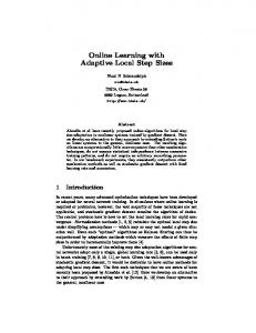
As we have seen, optimizing over a smaller sample can be beneficial (if we believe the significance of the bounds). But why chose a single sample size once and for all? A smaller sample set seems advantageous early on, but as an optimization algorithm approaches the empirical minimizer, it is hit by the statistical accuracy limit. This suggests that we should dynamically increment the size of the sample set. We illustrate this idea in Figure 2. In order to analyze such a dynamic sampling scheme, we need to relate the suboptimality on a sub-sample T to a suboptimality bound on S. We establish a basic result in the following theorem. Theorem 3. Let w be an (ǫ, T )-optimal solution, i.e. RT (w) − R∗T ≤ ǫ, where T ⊆ S, m := |T |, n := |S|. Then the suboptimality of w for RS is bounded w.h.p. in the choice of T as: ES [RS (w) − R∗S ] ≤ ǫ +

n−m H(m) . n

Proof. Consider the following equality (1)

For illustrative purposes, let us use the above result to select a sample size for SAGA, which yields the best guarantees. Proposition 2. Assume H(m) = D/m and n is given. Define C to be an upper-bound on CS , ∀S (from Lemma 1), n D then for m ≥ κ, V (m) := m + Ce− m provides a bound on the expected suboptimality of SAGA. It is minimized for the choice ) ( n ∗ . m = max κ, C log n + log D Proof. The first claim follows directly from the assumptions and Lemma 1. Moreover the tightest bound is obtained by differentiating V with regard to 1/m and solving for m (see Lemma 9 in appendix). The result implies that we will perform roughly log n + C log D epochs on the optimally sized sample. Also the value of the bound is (for simplicity, assuming C = D) 1 1 1 log n + ≤ V (n) = + , V (m ) = n n n e

(2)

(3)

RS (w) − R∗S = RS (w) ∓ RT (w) ∓ R∗T − R∗S

3.2. Sample Size Optimization

∗

(6)

We bound the three involved differences (in expectation) as follows: (2): RT (w) − R∗T ≤ ǫ by assumption. (3): ES [RT (wT∗ ) − RS (wS∗ )] ≤ 0 as T ⊆ S. For (1) we apply the bound (see Lemma 10 in the appendix) ES|T [RS (w) − RT (w)] ≤

n−m |R(w) − RT (w)| . n

Moreover ET [R(w)−RT (w)] ≤ sup |R(w′ )−RT (w′ )| ≤ H(m) w′

by Eq. (2), which concludes the proof. In plain English, this result suggests the following: If we have optimized w to (ǫ, T ) accuracy on a sub-sample T and we want to continue optimizing on a larger sample S ⊇ T , then we can bound the suboptimality on RS by the same ǫ plus an additional ”switching cost” of (n − m)/n · H(m).

4. Algorithms & Analysis (5)

1 The SAGA analysis holds for i.i.d. sampling, so strictly speaking this is not a pass, but corresponds to n update steps.

4.1. Computational Limited Learning The work of (Bottou, 2010) emphasized that for massive data sets the limiting factor of any learning algorithm will

R(w)

Starting Small – Learning with Adaptive Sample Sizes

H(n/4) H(n/3) H(n/2) H(n) sample size

Figure 2. Illustration of an optimal progress path via sample size adjustment. The vertical black lines show the progress made at each step, thus illustrating the faster convergence for smaller sample size.

Table 1. Comparison of obtained bounds for different SAGA variants when performing T ≥ κ update steps.

M ETHOD SAGA (one pass) SAGA (optimal size) DYNA SAGA

O PTIMIZATION ERROR

S AMPLES

const. O(log T · H(T )) O(H(T ))

T T / log T T /2

be its computational complexity T , rather than the number of samples n. For SGD this computational limit typically translates into the number of stochastic gradients evaluated by the algorithm, i.e. T becomes the number of update steps. One obvious strategy with abundant data is to sample a new data point in every iteration. There are asymptotic results establishing bounds for various SGD variants in (Bousquet & Bottou, 2008). However, SAGA and related algorithms rely on memorizing past stochastic gradients, cf. (Hofmann et al., 2015), which makes it beneficial to revisit data points, and which is at the root of results such as Lemma 1. This leads to a qualitatively different behavior and our findings indicate that indeed, the trade-offs for large scale learning need to be re-visited, cf. Table 1. 4.2. SAGA with Dynamic Sample Sizes We suggest to modify SAGA to work with a dynamic sample size schedule. Let us define a schedule as a monotonic function M : Z+ → Z+ , where t is the iteration number and M (t) the effective sample size used at t. We assume that a sequence of data points X = (x1 , . . . , xn ) drawn from P is given such that M induces a nested sequence of samples Tt := {xi : 1 ≤ i ≤ M (t)}.

Algorithm 2 DYNA SAGA 1: Input: training examples X = (x1 , x2 , . . . , xn ), xi ∼ P total number of iterations T (e.g. T = 2n) starting point w0 ∈ Rd (e.g w0 = 0) 1 learning rate η > 0 (e.g. η = 4L ) sample schedule M : [1 : T ] → [1 : n] 2: w ← w0 3: for i = 1, . . . , n do 4: αi ← ∇fxi (w0 ) {can also be done on the fly} 5: end for 6: for t = 1, . . . , T do 7: sample xi ∼ Uniform(x1 , . . . , xM(t) ) 8: g ← ∇fxi (wt−1 ) P 9: A ← M(t) j=1 αj /M (t) {can be done incrementally} 10: wt ← wt−1 − η (g − αi + A) 11: αi ← g 12: end for

DYNA SAGA generalizes SAGA (Defazio et al., 2014) in that it samples data points non-uniformly at each iteration. Specifically, for a given schedule M and iteration t, it samples uniformly from Tt , but ignores X − Tt . The pseudocode for DYNA SAGA is shown in Algorithm 1.

4.3. Upper Bound Recurrence We pursue the strategy of using the basic inequalities obtained so far and to stitch them together in the form of a recurrence. At any iteration t we allow ourselves the choice to augment the current sample of size m by some increment △m ≥ 0. We define an upper bound function U as follows   ρn U(t  − 1, n)  U(t, n) = min (7) n−m  min U(t, m) + n H(m) , m κ.

Proof. Here, we briefly state a sketch of the proof . The details are presented in Appendix A.2. First, we reformulate the problem of the optimal sample size schedule in terms of number of iterations on each samples size. Given that this problem is convex, we can use the KKT conditions to prove the optimality of incrementing by one sample (see Lemma 12) and iterating twice on each sample size (see Lemma 13).

5. Experimental Results We present experimental results on synthetic as well as real-world data, which largely confirms the above analysis.

Starting Small – Learning with Adaptive Sample Sizes −3

SGD SAGA dynaSAGA SSVRG SGD:0.05 SGD:0.005 SGD/SVRG

0

−4 −2 −5 −4 −6 −6

−7

−8

−8

−9 −10 −10 −12 −11

−12

0

0.5

1

1.5

2

2.5

3

3.5

4

−14

0

0.5

1

1.5

2

2.5

3

3.5

4

1. 0

4

4.5

5 4

x 10

x 10

2. A 9 A

RCV −2

0

−2 −2

−4 −4

−4

−6

−6 −6

−8

−8 −10

−8

−10

−12 −10 −14

−12

−12 −16

−14

0

1

2

3

4

5

6

7

8

9

−18

10

0

1

2

3

4

5

6

7

8

9

4

3.

10

−14

0

5

10

x 10

x 10

W8A

4.

−2

IJCNN 1

15 4

4

x 10

5.

REAL - SIM

0

−4 −5

−6

−8 −10 −10

−12 −15 −14

−16

−20

−18

−20

0

1

2

3

4

5

6

7

8

9

−25

10

0

1

2

3

4

5

6

5

6.

7

8

9

10 6

x 10

x 10

7. SUSY

COVTYPE

Figure 4.  Suboptimality on the empirical risk. The vertical axis shows the suboptimality of the empirical risk, i.e. log2 E10 RT (wt ) − R∗T where the expectation is taken over 10 independent runs. The training set includes 90% of the data. The vertical red dashed line is drawn after exactly one epoch over the data.

κ=

√

n

−3

l n[| R n ( w ) − R n ( w ∗ ) | ]

Suboptimality of Risk y = −0.59 x + −1.68

−4

−4

−5

−5

−6

−6

−7

−7

−8

−8

−9

−9

−10

−10

−11

−12

5.1. Baselines

κ = n0.75

−3 Suboptimality of Risk y = −1.04 x + 0.88

We compare DYNA SAGA (both the L INEAR and A LTER NATING strategy) to various optimization methods presented in Section 2. This includes SGD (with constant and decreasing step-size), SAGA, streaming SVRG (SSVRG) as well as the mixed SGD/SVRG approach presented in (Babanezhad et al., 2015).

−11

6

7

8

9

l n( n)

10

11

12

−12

6

7

8

9

10

11

12

l n( n)

Figure 3. Results on synthetic dataset. (left) Since, the empirical suboptimality is ∝ 1/n, we expect the slope measured on this plot to be close to one. (right) Since κ = n0.75 slows down the convergence rate, the slope of this plot is less than one.

5.2. Experiment on synthetic data We consider linear regression, where inputs a ∈ Rd are drawn from a Gaussian distribution N (0, Σd×d ) and outputs are corrupted by additive noise y = hx, w∗ i + ǫ,
2 ǫ ∼ N 0, σ . We are given n i.i.d observations of this

Starting Small – Learning with Adaptive Sample Sizes −2

SGD SAGA dynaSAGA SSVRG SGD:0.05 SGD:0.005 SGD/SVRG

0

−2 −4 −4 −6 −6

−8

−8

−10 −10 −12 −12 −14

−14

0

0.5

1

1.5

2

2.5

3

3.5

4

−16

0

0.5

1

1.5

2

2.5

3

3.5

4

1. 0

4

4.5

5 4

x 10

x 10

2. A 9 A

RCV −3

0

−4 −2

−5 −6 −5

−4

−7

−8

−6

−9 −10

−8

−10

−11 −10

−12

−15

0

1

2

3

4

5

6

7

8

9

10

−12

0

1

2

3

4

5

6

7

8

9

4

3.

−13

0

5

10

4.

IJCNN 1

15 4

x 10

x 10

W8A

−2

10 4

x 10

5.

REAL - SIM

0 −2

−4

−4 −6 −6 −8

−8

−10

−10 −12

−12

−14 −14 −16 −16

−18

−18

0

1

2

3

4

5

6

7

8

9

10

−20

0

1

2

3

4

5

6

5

6.

COVTYPE

7

8

9

10 6

x 10

x 10

7. SUSY

Figure 5. Suboptimality on the  expected risk. The vertical axis shows the suboptimality of the expected risk, i.e. log2 E10 RS (wt ) − RS (wT∗ ) , where S is a test set which includes 10% of the data and wT∗ is the optimum of the empirical risk on T . The vertical red dashed line is drawn after exactly one epoch over the data.

model, S = {(ai , yi )}ni=1 , from which we compute the P least squares risk RS (w) = n1 ni=1 (hai , wi − yi )2 .

By considering the matrix An to be a row-wise arrangement of the input vectors ai , we can write the Hessian matrix of Rn (w) as Σn = n1 ATn An . When n ≫ d, the matrix Σn converges to Σ and we can therefore assume that Rn (w) is µ-strongly convex and L-Lipschitz where the constants µ and L are the smallest and largest eigenvalues of Σ. We experiment with two different values for the condition number κ. √ Σ with elements deCase κ = n: We use a diagonal √ creasing from 1 to √1n , hence κ = n. In this particular case the analysis derived in Lemma 5 predicts an upper

bound U(n, n) < O( n1 ) which is confirmed by the results shown in Figure 3.
2 3 3 Case κ = n 4 : When κ = n 4 , the term nκ is the dominating term in the proposed upper-bound.   In this case, U(n, n) is thus upper-bounded by O √1n , which is once again verified experimentally in Figure 3. 5.3. Experiments on Real Datasets We also ran experiments on several real-world datasets in order to compare the performance of DYNA SAGA to stateof-the-art methods. The details of the datasets are shown in Table 2. Throughout all the experiments we used the lo-

Starting Small – Learning with Adaptive Sample Sizes

Table 2. Details of the real datasets used in our experiments. All datasets were selected from the LIBSVM dataset collection. DATASET RCV 1. BINARY A9A W8A IJCNN 1 REAL - SIM COVTYPE . BINARY

SUSY

S IZE 20242 32561 49749 49990 72309 581012 5000000

N UMBER OF

FEATURES

47236 123 300 22 20958 54 18

gistic loss with a regularizer λ = √1n 2 . Figures 4, and 5 show the suboptimality on the empirical risk and expected risk after a single pass over the datasets. The various parameters used for the baseline methods are described in Table 3. A critical factor in the performance of most baselines, especially SGD, is the selection of the step-size. We picked the best-performing step-size within the common range guided by existing theoretical analyses, specifically C for various values of C. Overη = 1/L and η = C+µt all, we can see that DYNA SAGA performs very well, both as an optimization as well as a learning algorithm. SGD is also very competitive and typically achieves faster convergence than the other baselines, however, its behaviour is not stable throughout all the datasets. The SGD variant with decreasing step-size is typically very fast in the early stages but then slows down after a certain number of steps. The results on the RCV dataset are somehow surprising as SGD with constant step-size clearly outperforms all methods but we show in the appendix that its behaviour gets worse as we increase the condition number. As can be seen very clearly, DYNA SAGA yields excellent solutions in terms of expected risk after one pass (see suboptimality values that intersect with the vertical red dashed lines).

6. Conclusion We have presented a new methodology to exploit the tradeoff between computational and statistical complexity, in order to achieve fast convergence to a statistically efficient solution. Specifically, we have focussed on a modification of SAGA and suggested a simple dynamic sampling schedule that adds one new data point every other update step. Our analysis shows competitive convergence rates both in term of suboptimality on the empirical risk as well as (more importantly) the expected risk in a one pass or a two pass setting. These results have been validated experimentally. Our approach depends on the underlying optimization 2 We also present some additional results for various regularizers of the form λ = n1p , p < 1 in the appendix

method only through its convergence rate for minimizing an empirical risk. We thus suspect that a similar sample size adaption is applicable to a much wider range of algorithms, including to non-convex optimization methods for deep learning.

References Babanezhad, Reza, Ahmed, Mohamed Osama, Virani, Alim, Schmidt, Mark, Koneˇcn`y, Jakub, and Sallinen, Scott. Stop wasting my gradients: Practical svrg. Advances in Neural Information Processing Systems, 2015. Bottou, L´eon. Large-scale machine learning with stochastic gradient descent. In Proceedings of COMPSTAT’2010, pp. 177–186. Springer, 2010. Boucheron, St´ephane, Bousquet, Olivier, and Lugosi, G´abor. Theory of classification: A survey of some recent advances. ESAIM: probability and statistics, 9:323–375, 2005. Bousquet, Olivier. Concentration inequalities and empirical processes theory applied to the analysis of learning algorithms. PhD thesis, Ecole Polytechnique, 2002. Bousquet, Olivier and Bottou, L´eon. The tradeoffs of large scale learning. In Advances in Neural Information Processing Systems, pp. 161–168, 2008. Boyd, Stephen and Vandenberghe, Lieven. Convex Optimization. Cambridge University Press, New York, NY, USA, 2004. Chandrasekaran, Venkat and Jordan, Michael I. Computational and statistical tradeoffs via convex relaxation. Proceedings of the National Academy of Sciences, 110 (13):E1181–E1190, 2013. Defazio, Aaron, Bach, Francis, and Lacoste-Julien, Simon. Saga: A fast incremental gradient method with support for non-strongly convex composite objectives. In Advances in Neural Information Processing Systems, pp. 1646–1654, 2014. Frostig, Roy, Ge, Rong, Kakade, Sham M., and Sidford, Aaron. Competing with the empirical risk minimizer in a single pass. In The Conference on Learning Theory, pp. 728–763, 2015. He, Xi and Tak´ac, Martin. Dual free SDCA for empirical risk minimization with adaptive probabilities. CoRR, abs/1510.06684, 2015. Hofmann, Thomas, Lucchi, Aurelien, Lacoste-Julien, Simon, and McWilliams, Brian. Variance reduced stochastic gradient descent with neighbors. In Advances in Neural Information Processing Systems 28, pp. 2296–2304. Curran Associates, Inc., 2015.

Starting Small – Learning with Adaptive Sample Sizes

Johnson, Rie and Zhang, Tong. Accelerating stochastic gradient descent using predictive variance reduction. In Advances in Neural Information Processing Systems, pp. 315–323, 2013. Kushner, Harold J and Yin, George. Stochastic approximation and recursive algorithms and applications, volume 35. Springer Science & Business Media, 2003. Moulines, Eric and Bach, Francis R. Non-asymptotic analysis of stochastic approximation algorithms for machine learning. In Advances in Neural Information Processing Systems, pp. 451–459, 2011. Polyak, Boris T and Juditsky, Anatoli B. Acceleration of stochastic approximation by averaging. SIAM Journal on Control and Optimization, 30(4):838–855, 1992. Robbins, Herbert and Monro, Sutton. A stochastic approximation method. The Annals of Mathematical Statistics, pp. 400–407, 1951. Roux, Nicolas L, Schmidt, Mark, and Bach, Francis R. A stochastic gradient method with an exponential convergence rate for finite training sets. In Advances in Neural Information Processing Systems, pp. 2663–2671, 2012. Schmidt, Mark, Roux, Nicolas Le, and Bach, Francis. Minimizing finite sums with the stochastic average gradient. arXiv preprint arXiv:1309.2388, 2013. Shalev-Shwartz, Shai and Zhang, Tong. Stochastic dual coordinate ascent methods for regularized loss. The Journal of Machine Learning Research, 14:567–599, 2013. Vapnik, Vlamimir. Statistical learning theory, volume 1. Wiley New York, 1998.

Starting Small – Learning with Adaptive Sample Sizes

A. Appendix A.1. Proofs Proof of Lemma 1. Proof. We start with the convergence rate of SAGA established in (Defazio et al., 2014) as    t 
|S| 0 ∗ 2 ∗ 2 t 0 ∗ 0 ∗ ∗ EA kw − wS k ≤ ρ|S| kw − wS k + RS (w ) − h∇RS (wS ), w − wS i − RS . µ|S| + L

(11)

We then use the L-smoothness assumption of fx (w) to relate the suboptimality on the function values to the bound in Eq. (11).       EA |RS (wt ) − RS (wS∗ )| = EA |Ex∈S fx (wt ) − Ex∈S [fx (wS∗ )] | L−smoothness   ≤ LEA kwt − wS∗ k2 11 ≤ ρt|S| CS ,

Eq.

where CS is the initial suboptimality on the empirical risk defined as:  
|S| RS (w0 ) − h∇RS (wS∗ ), w0 − wS∗ i − R∗S CS = L kw0 − wS∗ k2 + µ|S| + L

(12)

Note that this initial error depends on the set S and its size |S|. In the following Lemma, we propose an upper bound on this initial error that is independent of S Lemma 8. W.h.p, the initial suboptimality error of sample S is bounded by: CS ≤ ξ :=

 4L  R(w0 ) − R(w∗ ) µ

Proof. We first use the fact that RS (w) is µ-strongly convex as well as the optimality of wS∗ to bound CS as     |S| 0 ∗ 2 0 ∗ 0 ∗ ∗ CS := L kw − wS k + RS (w ) − h∇RS (wS ), w − wS i − RS (wS ) µ|S| + L   L |S|L  ≤ RS (w0 ) − RS (wS∗ ) + RS (w0 ) − h∇RS (wS∗ ), w0 − wS∗ i − RS (wS∗ ) µ µ|S| + L    |S|L  L RS (w0 ) − RS (wS∗ ) + RS (w0 ) − RS (wS∗ ) ≤ µ µ|S| + L (L>0) 2L   RS (w0 ) − RS (wS∗ ) ≤ µ   [1] [2] [3] 2L ≤ RS (w0 ) ∓ R(w0 ) ∓ R(w∗ ) ∓ R(wS∗ ) − RS (wS∗ ) µ We use the generalization bounds in (Vapnik, 1998) to upper bound [1] and [2]. For [3], we used the uniform convergence rate of the ERM that implies (Vapnik, 1998): R(wS∗ ) − R(w∗ ) ≤ c sup |RS (w) − R(w)|, w

where c is a constant. We then get w.h.p

CS ≤

 2L  H(|S|) + R(w0 ) − R(w∗ ) + cH(|S|) + H(|S|) . µ

(13)

Starting Small – Learning with Adaptive Sample Sizes

We also make the further assumption that with high probability the initial suboptimality is greater than a constant factor of the statistical accuracy, i.e. R(w0 ) − R(w∗ ) > (2 + c)H(|S|). We can then further upper bound CS as CS ≤

 4L  R(w0 ) − R(w∗ ) . µ

(14)

Lemma 9 (for Proposition 2). V (m) :=

n n D + Ce− m , then arg min V (m) = nC m log 0