State Estimation and Mean Field Control with ... - Semantic Scholar

1

State Estimation and Mean Field Control with Application to Demand Dispatch

arXiv:1504.00088v1 [cs.SY] 1 Apr 2015

Yue Chen, Ana Buˇsi´c, and Sean Meyn

Abstract—This paper concerns state estimation problems in a mean field control setting. In a finite population model, the goal is to estimate the joint distribution of the population state and the state of a typical individual. The observation equations are a noisy measurement of the population. The general results are applied to demand dispatch for regulation of the power grid, based on randomized local control algorithms. In prior work by the authors it has been shown that local control can be carefully designed so that the aggregate of loads behaves as a controllable resource with accuracy matching or exceeding traditional sources of frequency regulation. The operational cost is nearly zero in many cases. The information exchange between grid and load is minimal, but it is assumed in the overall control architecture that the aggregate power consumption of loads is available to the grid operator. It is shown that the Kalman filter can be constructed to reduce these communication requirements, and to provide the grid operator with accurate estimates of the mean and variance of quality of service (QoS) for an individual load.

I. I NTRODUCTION Mean field games are a valuable tool for design and performance approximation for certain classes of interacting systems [1]–[3]. The infinite-population mean-field equations provide tremendous insight, but ultimately we must translate this insight to address a finite-population reality. In this paper we propose algorithms based on the Kalman filter to obtain estimates of first and second order statistics of the population and a typical individual, based on noisy observations of the population. While the potential applications are far broader than power systems, for ease of exposition it is convenient to restrict attention to one application. Renewable energy sources such as wind and solar power have a high degree of unpredictability and time variation, which makes balancing demand and supply more challenging. One possible way to address this challenge is to harness the inherent flexibility in demand of many types of loads. Demand Response is traditionally meant as a reduction in load in response to some grid-level event. It is in use today for peak-shaving (smoothing demand), and for contingency reserves (load-shedding following generation loss). It is argued in [4]–[6] that the value of demand-side flexibility is far greater than this. Loads can supply a range of grid services, such as the balancing reserves required at BPA, or Research supported by NSF grants CPS-0931416 and CPS-1259040, and the French National Research Agency grant ANR-12-MONU-0019 Y.C. and S.M. are with the Department of Electrical and Computer Engg. at the University of Florida, Gainesville. A.B. is with Inria and the Computer ´ Science Dept. of Ecole Normale Sup´erieure, Paris, France.

the Reg-D/A regulation reserves used at PJM [5]. These grid services can be obtained without impacting quality of service (QoS) for consumers [3], [7]. This is only possible through design. The term Demand Dispatch, introduced in [8], is used to emphasize the difference between the goals of our own work and traditional demand response. The application in this paper concerns a large collection of loads whose power consumption is not continuously variable. Examples include thermostatically controlled loads, as considered in [2], and irrigation or pool-pumps [3], [6]. In these papers and [9] it is argued that randomization at the load is valuable to avoid synchronization, and to simplify control at the grid level. A mean-field model is obtained for control at the grid level: The control solution adopted in [2] is based on state-feedback for a linear state space model with partial observations. The system is in fact bi-linear, and represented as a linear model by treating the product of inputs and states as a new input. This is why state estimation is needed for implementation of the algorithm. In [6] a randomized policy is designed for each load so that the aggregate input-output system is easily controlled without the use of state estimates. For simplicity, in this paper we restrict attention to the setting of [6], in which each load evolves as a controlled Markov chain. The transition probability is determined by its own state, and a scalar signal ζ broadcast from a balancing authority (BA). The extension to vector inputs, as in [2], requires only changes in notation. The common dynamics are defined by a controlled transition matrix {Pζ : ζ ∈ R}. For the ith load, there is a state process X i whose transition probability is defined by, i Pζ (x− , x+ ) = P{Xt+1 = x+ | Xti = x− , ζt = ζ}

(1)

where x− and x+ are possible state-values. In the case of a water heater, the state x ∈ X might represent temperature of the water, and whether the unit is operating or not. If there are N loads operating independently, conditional on the common signal ζ, then the empirical distribution (i.e., the histogram of state values) is defined as the average, µN t (x) =

N 1 X I{Xti = x} , N i=1

x∈X

Viewed as a row vector, the following recursion is central to the analysis in [3], [6]: N µN t+1 = µt Pζt + Wt+1 ,

(2)

where {Wt : t ≥ 1} is a martingale-difference sequence (and hence uncorrelated). In this paper we will have an observation

2

model that is also linear in the state, X Yt = µN t (x)U (x) + Vt

(3)

x

where U : X → R, and {Vt : t ≥ 1} is an uncorrelated sequence that is also uncorrelated with {Wt : t ≥ 1}. We develop the Kalman filter in two settings: In the first, we obtain estimates of µN t given the observations. The second filter obtains estimates of the joint statistics of a larger state that includes both µN t and the state of a typical individual. The main conclusions are summarized here: (i) A measurement architecture is proposed in which loads broadcast their state only occasionally - say, once per day. The observation equations in the aggregate model then include white noise, whose conditional variance is computed. The state equations for the population/individual dynamics evolve as a linear stochastic system with white noise disturbance, whose conditional covariance matrix is also computable. These conditional second-order statistics are the parameters required to define the Kalman filter. (ii) In the examples considered, the observability Grammian is not full rank, and an approximate time-invariant model is also unobservable. It is shown that the Kalman filter remains valuable for reducing the impact of measurement noise, and for estimating the distribution of quality of service. In particular, we find that estimates of some first and second order statistics of an individual load are remarkably accurate, even though the measurements are a noisy sequence of samples from the population. (iii) In the face of un-modeled dynamics such as load heterogeneity, or additional “opt-out” control used to enforce QoS bounds, the Kalman filter combined with PI control continues to perform nearly perfectly, even with 0.1% sampling of loads. There are in fact two general formulations of the Kalman filter. In the first, most typical setting, the sequence of Kalman gains is deterministic; obtained through a Riccati equation (a recursive equation driven by the covariance matrices for the state and observation noise). This is known to be L2 -optimal over all estimators that are linear functions of the observations. A second formulation of the Kalman filter uses conditional covariance matrices to define the Kalman gain. If the state/observation noise is conditionally Gaussian, then this Kalman filter coincides with the nonlinear filter, which is L2 optimal over all causal estimators [10]. Because the Riccati equation is a nonlinear function of the covariance matrices, this version of the Kalman filter may be a nonlinear function of the observations. In this paper we consider both forms. The second is attractive because it is easy to compute formulae for the conditional covariance matrices, while the unconditional covariance matrices only admit approximations. Moreover, when considering the dynamics of the aggregate, a Gaussian approximation of the noise is justified by the Central Limit Theorem (CLT).

Related research: Besides the references cited above, there are many papers on demand dispatch based on centralized control, or relying on real-time prices to solve the control problem of interest. Much of the latter is closer to demand response, and has little intersection with the research summarized here. An application of this formulation of the Kalman filter was considered previously in [11] for a single Markov chain without control, with measurements subject to Gaussian error. There are several recent papers with similar goals in the mean-field games literature. Most closely related is [12] which concerns partially observed LQG mean field games, with several classes of players. The state estimation problem is from the point of view of the individual – each “minor agent” obtains noisy and partial observations, and wishes to estimate the “major state” as well as the aggregate. The solution is obtained through the construction of a Kalman filter. This prior work is also motivated by application to power systems. The remainder of the paper consists of four sections organized as follows. The following section describes the stochastic model on which the estimation algorithms are based. The focus here and throughout the paper is on applications to demand dispatch; the section closes with a variant of the example of [6]. Filtering equations are derived in Section III. The state equations and conditional covariance matrices required to construct a Kalman filter are derived in two general settings. The algorithms have been tested in various different settings – results are summarized in Section IV. Conclusions and directions for future research are contained in Section V. II. M EAN F IELD M ODEL It is assumed throughout the paper that a family of Markov transition matrices {Pζ : ζ ∈ R} is given that in continuous in the parameter ζ. The finite state space is denoted X = {x1 , . . . , xd }, so that each Pζ is a d × d matrix. The mean-field model is defined as the approximation of (2) obtained as N → ∞. This is the deterministic recursion, µt+1 = µt Pζt ,

(4)

with µ0 given, and where ζ is obtained via causal feedback. This paper is concerned with the stochastic system (2), but the steps used to justify the limit will lead to the second-order statistics required to describe the Kalman filter. A. Aggregate dynamics The individual dynamics are described by the controlled Markov model (1). We lift the state space from the d-element set X = {x1 , · · · , xd }, to the d-dimensional simplex S. For the ith load at time t, the element Γit ∈ S is the degenerate distribution whose mass is concentrated at x if Xti = x; that is, Γit = δx . These distributions evolve according to a random linear system, Γit+1 = Γit Git+1 (5) in which Γit is interpreted as a d-dimensionalProw vector, Git is a d × d matrix with entries 0 or 1 only, and l Git (xj , xl ) = 1 for all j.

3

The statistics of the noise in the measurement equation (3) will be described in the next section. We denote the filtration of observations by, Yt = σ{Yr , ζr : r ≤ t},

t ≥ 0.

ζt = φt (Y0 , . . . , Yt ) A2: For some function Ξ with domain R×[0, 1], and range equal to the set of d × d matrices, (7)

where {ξti : t ≥ 1, i ≥ 1} are i.i.d. on [0, 1]. A3: The initial conditions {Γi0 : 1 ≤ i ≤ N } are i.i.d., with P{Γi0 (x) = 1} = µ0 (x), x ∈ X A4: The measurements are obtained through sampling: There is a bounded sequence {γt : t ≥ 1} of N dimensional vectors with non-negative entries, and independent of the {ξti }, such that E[γt (k)] = N −1 for each t and k, and Yt =

N X

γt (i)U (Xti ).

i=1

Moreover, the distribution of γ is unchanged by permutations of its N components. Assumption A4 can be used to model random sampling with or without replacement. Under A1–A3, Git+1 is conditionally independent of {Γi0 , · · · , Γit }, given Yt , with E[Git+1 | Yt ] = Pζt .

(8)

Two filtering problems are considered in this paper. In the first, the state is equal to the empirical distributions expressed as column vectors: k Φt (k) = µN t (x ),

1 ≤ k ≤ d, t ≥ 0.

(9)

In the second, the goal is to estimate the state for an individual load. For the ith load we denote, Φit (k) = Γit (xk ),

1 ≤ k ≤ d, t ≥ 0.

Wt+1

(6)

The following assumptions are imposed throughout: A1: For a continuous family of functions φt : Rt+1 → R, we have for each t,

Git = Ξ(ζt−1 , ξti ),

where At = PζTt , and for each i, t,

i Wt+1

1 N

Φit

Yt = CΦt + Vt

Φit+1

i

=

At Φit

+

i Wt+1

t u

It follows from (8) that W is a martingale difference sequence, as is the average W . Consequently, the state noise is uncorrelated. A derivation of the conditional state covariances are given in Section III-A. For a linear-Gaussian model, the Kalman filter equations are intended to approximate the conditional mean and covariance of the state. In the first model (12) they are denoted, b t = E[Φt | Yt ] , Φ

e tΦ e Tt | Yt ] Σt = E[Φ

(17)

e t = Φt − Φ b t . In the examples to be considered, with Φ for large N it can be argued via the CLT that (V , W ) is approximately conditionally Gaussian given the observations. We might expect the Kalman filter to approximate the optimal nonlinear filter in this case. In Section III-C we extend the state space to obtain estimates of QoS metrics for an individual load that may not be a function of the respective state Φit . B. Example: Intelligent pools In this paper we focus on a single example in which each load is a residential pool pump. In the full journal version of the paper we will discuss other applications. In the original model of [6], the state space is taken to be the finite set, X = {(m, k) : m ∈ {⊕, }, k ∈ {1, . . . , I}}

(18)

where I > 1 is an integer. If Xti = (⊕, k), this means that the pool pump is on at time t, and has remained on for the past k time units. In this paper we take the same state space, but with a new interpretation of each state. 1

...

2

On

...

I −1

I

2

1

(11)

i=1

= At Φt + Wt+1

(16)

where CΦt = µN (U ). That is, Ci = U (xi ) for each i.

(10)

In each case, the observation equation is (3), where U (x) represents power consumption of a load when its state is x. The following result follows from the definitions, and is also the basis of the analysis in [3]: Proposition 2.1: The two state processes each evolve as linear systems, Φt+1

(15)

...

Φt =

(14)

The observation equation (3) can be written,

The two state processes are evidently related, N X

N 1 X k Wt+1 N k=1  T = Γit (Git+1 − Pζt )

=

(12) (13)

I Fig. 1.

I −1

...

State transition diagram for pool pump model.

The local policy introduced here involves an additional layer of randomness for each load. Its definition requires a controlled transition matrix denoted Pˇζ , and a parameter δ ∈ (0, 1). At each time t, a weighted coin is flipped with probability of heads equal to δ. If the outcome is a tail, then the state does not change. Otherwise, a transition is made from the

4 10 5

Pζ = (1 − δ)I + δ Pˇζ

Output deviation

10 -10 43

96

i

Estimate

Mean

40

Empirical

Lt

20 0

−20 6

Variance 60

80

100 t/hour

120

140

160

Input ζt

5 0 −5

40

23

Fig. 3. Observability Grammian for the pool pump model: The magnitude of eigenvalues decays rapidly for a typical sample-path of ζ, and for the LTI model obtained with ζ ≡ 0.

ΣL t

4 2 0 0

20

λζ

−∞

Reference

0

-10 0

λ

10 -5

0

×10 3

kW

10

10 0

(19)

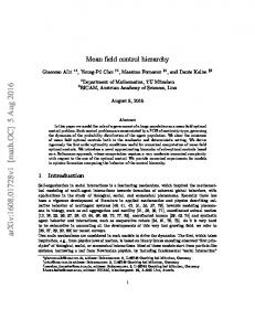
A state transition matrix is shown in Fig. 1. The motivation comes from conflicting needs of the grid and the load: a single load turns on or off only a few times per day, yet the grid operator wishes to send a signal far more frequently – In this example we assume every 5 minutes. If the sampling increments for each load were taken to be 5 minutes, then it would be necessary to take I very large in the approach of [6]. In this paper Pˇζ is obtained using the optimal-control approach of [6]; we take I = 48, and hence d = |X| = 96. It is assumed that δ = 1/6, so that the pool state changes every 30 minutes on average.

96 Eigenvales of the Observability Grammian

log(|λi |)

current state x to a new state x+ with probability Pˇζ (x, x+ ). The overall transition matrix is thus

Fig. 2. The deviation in power consumption tracks well even with only 20 pools engaged.

For sake of illustration, Fig. 2 shows tracking performance of this scheme with only twenty pools. Each pool is assumed to consume 1 kW when operating, and each has a 12 hour cleaning cycle. The grid operator uses PI compensation to determine ζ (see [6] for details). With such a small number of loads it is not surprising to see some evidence of quantization. For 100 loads or more, and the reference scaled proportionately, the tracking is nearly perfect. Two QoS metrics have been considered for this model. First is ‘chattering’ – a large number of switches from on to off. A large value means poor QoS, but this is already addressed through the design of Pˇζ . The design also helps to enforce upper and lower bounds on the duration of cleaning each day. A second metric is total cleaning over a time horizon of one week or more. In [3] the following indicator of QoS is investigated: t X Lit = `(Xti ) (20) k=0

where the function ` depends only on the on/off component of the state, with steady-state mean equal to zero for the nominal model (with ζ ≡ 0). The function `(x) = I(m = ⊕) − I(m = ) was used in [3] in the case of a 12 hour cleaning cycle (recall the notation x = (m, k)). In anticipation of the results to come we ask, what would linear systems theory predict with respect to state estimation performance? We computed the observability Grammian associated with (12) for typical sample paths {At = PζTt : 1 ≤ t ≤ 2016}, where the value 2016 corresponds to one

100

200

300

400

t/hour

500

600

700

Fig. 4. Although the liner model is not observable, estimates of the mean and variance of QoS for an individual are nearly perfect.

week, and ζ was scaled to lie between ±1/2. Its rank was found to be approximately 40, while the maximal rank is 96 (the dimension of the state). With ζt ≡ 0 the system is time-invariant. In this case the rank of the observability Grammian coincides with the rank of the observability matrix, which was found to be 23. Fig. 3 shows a plot of the log of the magnitude of the eigenvalues for the two observability Grammians. The rank of 43 indicated in the figure was obtained in one experiment for the time-varying system. Fig. 4 shows estimates of QoS based on a model with 10,000 pools, with only 10 of the pools sampled at each time instance (the average of these ten values defines the observation equation (3)). The accuracy of estimation is remarkable, in spite of significant measurement noise. More details can be found in Section IV. Conclusion: Estimation of important metrics is possible with significant measurement noise, even though the linear model is highly unobservable. III. K ALMAN F ILTER E QUATIONS In this section we derive formulae for the second order statistics for the disturbances appearing in the linear model (12, 12, 16). These expressions are used to construct a Kalman filter that generates approximations for the conditional mean and covariance (17). Other statistics of interest are, b it = E[Φit |Yt ] , Φ

e it (Φ e it )T |Yt ] Σit = E[Φ

i bi Φ t+1|t = E[Φt+1 |Yt ] ,

e it+1 (Φ e it+1 )T |Yt ] Σit+1|t = E[Φ

b t+1|t = E[Φt+1 |Yt ] , Φ

e t+1 (Φ e t+1 )T |Yt ] Σt+1|t = E[Φ

5

e it = Φit − Φ b it . where again tildes represent deviations, such as Φ Prop. 3.1 states that some statistics of the individual can be expressed in terms of those of the population: It is not the case that Σit = N Σt , since {Φit : 1 ≤ i ≤ N } are correlated. Proposition 3.1: For each s, t, i, and any set S ⊂ Rd , the conditional probability is independent of i: P{Φis ∈ S | Yt } = P{Φ1s ∈ S | Yt }

(21)

and consequently, E[Φis | Yt ] = E[Φs | Yt ]. Moreover, bi b Φ t+1|t = At Φt , the state covariances for the individual are b t) − Φ b tΦ b Tt Σit = diag (Φ b t+1|t ) − Φ b t+1|t Φ bT Σit+1|t = diag (Φ t+1|t ,

Proof: Since {Wti : 1 ≤ i ≤ N } is uncorrelated, ΣW t =

t+1|t

Proof: The proof of (21) follows from the symmetry and independence conditions imposed in (A1–A4). The remaining results follow from this, and the fact that Φit has binary entries [in particular, Φit (Φit )T = diag (Φit )]. Recall from the introduction that two formulations of the Kalman filter are considered in this paper. For a conditionally Gaussian model, the Kalman filter equations require the conditional covariances for the state noise,

b it = Φ b t , and from this or (11) it Moreover, Prop. 3.1 gives Φ is obvious that N X bi bt = 1 Φ Φ N i=1 t Consequently, (25) follows from (26). i The derivation of the formula (26) for ΣW is similar to the t Kalman filter construction in [11]. Consider first the larger sigma-field,

We compute the conditional covariance given Yt+ , and then use smoothing:   i i i ΣW = E E[Wt+1 (Wt+1 )T | Yt+ ] | Yt t From the definition (15), we must compute the conditional covariance of Φit+1 given Yt+ . That is, i i E[Wt+1 (Wt+1 )T | Yt+ ]

= E[Φit+1 (Φit+1 )T | Yt+ ]

− E[Φit+1 | Yt+ ]E[Φit+1 | Yt+ ]T

= diag (At Φit )

− At diag (Φit )ATt

i

i i T ΣW = E[Wt+1 (Wt+1 )T | Yt ] , ΣW t t = E[Wt+1 Wt+1 | Yt ] (22) and also the conditional covariance of the measurement noise,

(23)

Formulae for the state noise covariances can be obtained in full generality. We require the distribution of the random vector γt introduced in A4 to obtain a formula for ΣVt . The Kalman filter that generates L2 -optimal estimates over all linear functions of the observations uses instead the (unconditional) covariance matrices, Wi

Σt

i i = E[Wt+1 (Wt+1 )T ],

W

T Σt = E[Wt+1 Wt+1 ],

(27)

Yt+ = σ{Φir , Yr , ζr , Ar : r ≤ t, i ≤ N }

and the cross covariances can be expressed,  i  e t (Φ e t )T | Yt = Σt E Φ  i  e e t+1|t )T | Yt = Σt+1|t , 1 ≤ i ≤ N. E Φ (Φ

2 ΣVt = E[Vt+1 | Yt ]

N 1 X Wi Σ N 2 i=1 t

(24)

V

2 and Σt = E[Vt+1 ].

A. State noise covariance The following result provides formulae for the conditional covariances for the state noise (22) as a function of the b t. conditional mean Φ Proposition 3.2: Under Assumptions A1–A4,  1 T b b ΣW = diag (A Φ ) − A diag ( Φ )A (25) t t t t t t N i b it ) − At diag (Φ b it )ATt ΣW = diag (At Φ (26) t The second covariance is independent of i, with common value i ΣW = N ΣW t t .

where the final equation uses E[Φit+1 | Yt+ ] = At Φit , and the fact that Φir has binary entries for each i and r. Taking the conditional expectation given Yt gives (26). B. Sampling and observation covariance The observation model used in our numerical experiments is based on random sampling of loads: An integer n < N is held fixed, and at each time instant t wePchoose at random n indices n {k1 , . . . , kn } and take Yt = n−1 i=1 U (Xtki ). Recalling the ki ki definition U (Xt ) = CΦt , it follows from Prop. 3.1 that this is an unbiased estimate of CΦt . We obtain here an expression for the conditional variance ΣVt defined in (23). Proposition 3.3: The conditional covariance is given by,  1 N −n  i ΣVt = C Σt+1|t − Σt+1|t C T n N −1 Proof: By definition, ΣVt = E

n h 1 X

n

i=1

i CΦkt+1 − CΦt+1

2

| Yt

i

where the permutation is random, uniform, and independent of Yt . It follows from symmetry of the model that we can consider just the first n samples, replacing ki by i. We also center the random variables to obtain n h 1 X 2 i ei e t+1|t | Yt ΣVt = E CΦ − C Φ (28) t+1|t n i=1

6

We expand the quadratic to obtain the sum of three terms. One is the conditional variance, 
 e t+1|t 2 | Yt = CΣt+1|t C T S1 := E C Φ (29) The remaining steps use the following consequence of Prop. 3.1:   T e ei E {C Φ (30) t+1|t }{C Φt+1|t } | Yt = CΣt+1|t C The cross term is transformed using this identity: n h 1 X   i ei e t+1|t | Yt CΦ C Φ S2 := E t+1|t n i=1 = CΣt+1|t C

(31)

T

The third term is another conditional variance, n 2 i 1 hX e i S3 := 2 E C Φt+1|t | Yt n i=1 =

n  1 X  ei ej E {C Φt+1|t }{C Φ } | Yt t+1|t 2 n i,j=1

Applying symmetry once more gives, n X   ei ej E {C Φ t+1|t }{C Φt+1|t } | Yt

i,j=1

  2 e1 = nE {C Φ t+1|t } | Yt   e1 e2 + (n2 − n)E {C Φ t+1|t }{C Φt+1|t } | Yt Using familiar arguments, and applying (30),   e1 e2 (N − 1)E {C Φ t+1|t }{C Φt+1|t } | Yt =

N X   e1 ek E {C Φ t+1|t }{C Φt+1|t } | Yt

k=2

  e1 e = N E {C Φ t+1|t }{C Φt+1|t } | Yt   e1 − E {C Φ }2 | Yt

We adopt the following generalization of (20): We assume that P0 has a unique invariant probability measure π0 . With ` : X → R a given function with zero steady-state mean, P x π0 (x)`(x) = 0, we define for each i and t, Lit =

= N CΣt+1|t C −

CΣit+1|t C T

Putting these expressions together gives, i n2 − n h 1  N Σt+1|t − Σit+1|t C T S3 = 2 C nΣit+1|t + n N −1 The expansion of the quadratic (28) results in ΣVt

= S1 − 2S2 + S3 ,

so the desired expression is obtained by simplifying this sum.

C. Estimation of the individual We now construct a filter to estimate the mean and covariance of the individual state Φi . We also seek estimates of the mean and variance of a particular formulation of QoS for a typical load. Estimates of the individual state and individual QoS can be used to estimate the flexibility of loads, which may vary with time. For example, if the grid operator believes that every water heater contains water that is too cold, then it is unlikely that there is much remaining flexibility to reduce power consumption from these loads.

β t−k `(Xki )

(32)

k=0

with β ∈ (0, 1] a constant. In the pool model this was described previously, this is a measure of under- or overcleaning over a long time-horizon. In other examples it might measure the level of “chattering” — the number of state changes from on/to off for a pool or water heater. In [3] an additional layer of control is introduced: The load can opt-out of service to the grid (ignore the signal ζt ) at any time t for which Lit lies outside of pre-assigned bounds. The case β = 1 was chosen so that the pair (Xti , Lit ) could be modeled as a controlled Markov chain on a finite state space. This is useful for computing or approximating the proportion of loads that opt-out. It was observed in simulation that the capacity of ancillary service to the grid is reduced with the introduction of this extra layer of control, but this is insignificant if the proportion of loads opting out is small. The Kalman filter must be modified to obtain estimates of the QoS for individual loads. One approach is to restrict to β = 1, and use the Markovian model (Xti , Lit ). This comes with high complexity: In the case of the pool model, the first component can take on d = 96 values, and the range of values of Lit may be over 100. This means that the state space is at least 104 , which is probably too large to be practical for estimation. Here we introduce a Kalman filter for the joint process Ψit = (Φit ; Φt ; Lit ), which is of dimension 2d + 1. The construction of a linear model for Ψi is based on (12, 13), and the onedimensional dynamics for QoS, Lit+1 = βLit + C` Φit

t+1|t T

t X

where C` Φit = `(Xti ). The measurements remain of the form (3), which is why it is necessary to include Φt in the definition of Ψit . The new A, C, state-noise covariance matrices are, 

At 0 C`

0 At 0

 0 0 , β

 [0, C, 0] ,

i

ΣW t N −1 ΣW i t 0

N −1 ΣW t ΣW t 0

i

 0 0 0

We thus have all of the system parameters needed to construct the Kalman filter. IV. E STIMATING Q O S AND C LOSING THE L OOP We have conducted experiments in various settings, using both formulations of the Kalman filter. For estimating performance we obtained excellent results with the Kalman filter whose gain is based on the conditional covariance matrices. In applications of the linear formulation of the Kalman filter we require the unconditional covariances. The state covariance matrix could be obtained as the mean of (25): i 1 h W b t ) − At diag (Φ b t )ATt Σt = E diag (At Φ N

7

b t ] = E[Φt ] does not have a closed form The mean E[Φ expression, so we make two approximations. First, we consider the mean with ζ ≡ 0, and second we let t → ∞. The covariance used in the filter is the resulting limit, i 1h W Σ∞ = (33) diag (At π0 ) − At diag (π0 )ATt N where π0 is invariant for P0 . A similar approximation is used V for Σt . The common features in all of the numerical experiments that follow are listed here: The reference signal r was generated from the BPA balancing reserves deployed in the first week of 20151 . This signal was low pass filtered, and then scaled to an appropriate magnitude to match the capacity of the aggregate of loads [6]. In the few cases where we required more than one week of data we simply cascaded this signal. The observation model was based on sampling: At each time, the grid operator obtains measurements randomly from 0.1% of the pools; it is assumed that each pool pump consumes 1kW while in operation. The average of these samples at time t is denoted Yt . The actual power consumption at time t is N CΦt . For this b t are scaled by N to represent reason, plots of CΦt or Ybt = C Φ total power consumption or its estimate. Finally, the discount factor β in the QoS metric (32) was chosen as the value for which β k ≈ 1/2 when k corresponds to one week. The value β = 0.9997 is obtained under the assumption of five-minute sampling. A. Estimation of QoS The Kalman filter described in Section III-C was used to obtain estimates of the mean and variance of the QoS metric Lit , with `(x) = Cx − y. Experiments were conducted on 10,000 pools with a 12hr/day cleaning cycle (so that y = 1/2). These experiments were performed with ζ equal to the exogenous “mean-field limit” used in the linearized model of [3]: Gc ζt = rt 1 + Gc Gp where Gc is a PI compensator, and Gp is a transfer function for a linearized model. As seen in Fig. 4, the empirical mean and variance of QoS were successfully estimated with negligible error. B. Heterogeneous population Here we summarize results from closed-loop experiments in which un-modeled dynamics are present due to load heterogeneity and opt-out control. With large un-modeled dynamics it is still possible to obtain estimates of the mean of QoS, but the Kalman filter cannot be expected to provide estimates of the variance. Error feedback was used in all of the remaining experiments, ζt = Gc et . A PI compensator was used to define Gc : A proportional gain of 50, and integral gain of 1.5 worked well in all examples. In the experimental results illustrated 1 http://tinyurl.com/BPAbalancing

in Fig. 5, the error signal was defined with respect to the raw measurements, without use of the Kalman filter. In all other experiments, the following definition was used: 1 bt − y rt − Yet , Yet = C Φ (34) N with y equal to the average nominal power consumption. The b t is an scaling of the reference by N −1 is required since C Φ estimate of average power consumption. The simulation model used in the remaining experiments consisted of nine different classes of pools, distinguished by their cleaning cycle. The total number of pools was taken to be 300,000. The distribution of classes is shown in Table I. Suppose that the grid operator had full information regarding the number of pools in each class. The full state space description would have dimension 9 × d, which is far too complex. Moreover, in practice the grid operator will not have complete system information. Here we make some coarse approximations to simplify the model. In addition to reducing complexity of the filter, our goal is to investigate robustness of the estimation algorithms in a closed-loop setting. et =

TABLE I: D ISTRIBUTION OF POOLS Cycle (hr/day)

20

18

16

14

12

10

8

6

4

Number (×104 )

1

1

1

3

5

10

5

3

1

Although the simulation uses these nine classes of pools, we obtain an approximate model based on just two pool models, corresponding to 8 and 12-hour cleaning cycles. Following [2], we fix a parameter 0 ≤ α ≤ 1, and define At = αA8t + (1 − α)A12 t 8

W ΣW + (1 − α)ΣW t = αΣt t

12

where the superscripts 8 and 12 refer to the respective pool classes. The parameter α was chosen to be consistent with the hypothesis that the collection of pools consist of just two classes, with 8 or 12 hr/day cycles. It is assumed that the nominal average power consumption y is known to the grid operator – this can be estimated easily from weekly measurements. The 2-class assumption would imply that y = αy 8 + (1 − α)y 12 , giving α = (y 12 − y)/(y 12 − y 8 ), with y 12 = 1/2 and y 8 = 1/3. With such large un-modeled dynamics, it is reasonable to increase the state noise covariance: W

W∗ ΣW + kt Σ ∞ , t = Σt

(35)

∗ where, kt ≥ 0, the conditional covariance ΣW is a convex t W combination of the matrices computed in Prop. 3.2, and Σ∞ is given in (33). In these experiments kt = 600. With the experimental setting fully described, we now describe results from several control experiments. We first show what happens if we forgo use of the Kalman filter, and take et = N −1 rt − Yet , with Yet = Yt − y, and Yt the noisy measurements obtained with 0.1% sampling. Results

8

Output deviation

100

V. C ONCLUSIONS

Reference

The construction of a Kalman filter for the joint population/individual dynamics is possible, and its performance is Reference

Output deviation

0 100

0

0

20

Fig. 5.

40

60

80

t/hour

100

120

140

160

−10

50 0

−50

PI control with output-error feedback, with et = N −1 rt − Yt .

from one experiment are shown in Fig. 5. The volatility of the measurements resulted in similar volatility of input ζt . This drove the pools to switch frequently, and also resulted in degraded grid level tracking. This result motivates the use of a filter to smooth the measurements. Results using the filtered error (34) are shown in Fig. 6. This Kalman filter estimator based control gives nearly perfect tracking performance, in spite of the significant modeling error.

0.5 0.25

−100 0

Fig. 7.

20

40

60

80

t/hour

100

120

140

160

Opt-out %

10

−100

Input ζt

−50

MW

MW

50

PI control with heterogeneity and opt-out local control

remarkable in the test cases considered. In particular, it is very surprising to obtain accurate tracking of both the mean and variance of QoS for an individual, given extremely noisy estimates of the population. We are currently considering other applications, and further analysis to gain insight on estimation performance.

Reference

Output deviation

R EFERENCES

100

MW

50 0

−50 −100 0

Fig. 6.

20

40

60

80

t/hour

100

120

140

160

PI control with smoothed error signal (34).

C. Opt-out local control We now introduce local opt-out control, introducing additional un-modeled dynamics. At each load the QoS metric Lit is constrained to a common interval [−50, +50]: if Lit ≥ 50, then the pool is turned off at time t, regardless of the value of ζt . Similarly, if Lit ≤ −50 then it will be turned on. In the construction of the Kalman filter, the state noise covariance was taken as (35), but in this case the scaling factor was chosen as a function of the QoS estimates, kt = k + b|Lbit | This is chosen to reflect the fact that un-modeled dynamics increase with the percentage of pools that opt-out. The values k = 3000 and b = 300 worked well, and the sensitivity to these values was not high. Closed loop results are shown in Fig. 7. The performance remains nearly perfect, and the percentage of opt out loads is less than about 0.5% throughout the run.

[1] M. Huang, P. E. Caines, and R. P. Malhame, “Large-population costcoupled LQG problems with nonuniform agents: Individual-mass behavior and decentralized ε-Nash equilibria,” IEEE Trans. Automat. Control, vol. 52, no. 9, pp. 1560–1571, 2007. [2] J. Mathieu, S. Koch, and D. Callaway, “State estimation and control of electric loads to manage real-time energy imbalance,” IEEE Trans. Power Systems, vol. 28, no. 1, pp. 430–440, 2013. [3] Y. Chen, A. Buˇsi´c, and S. Meyn, “Individual risk in mean-field control models for decentralized control, with application to automated demand response,” in Proc. of the 53rd IEEE Conference on Decision and Control, Dec. 2014, pp. 6425–6432. [4] D. Callaway and I. Hiskens, “Achieving controllability of electric loads,” Proceedings of the IEEE, vol. 99, no. 1, pp. 184 –199, jan. 2011. [5] P. Barooah, A. Buˇsi´c, and S. Meyn, “Spectral decomposition of demandside flexibility for reliable ancillary services in a smart grid,” in Proc. 48th Annual Hawaii International Conference on System Sciences (HICSS), Kauai, Hawaii, 2015. [6] S. Meyn, P. Barooah, A. Buˇsi´c, Y. Chen, and J. Ehren, “Ancillary service to the grid using intelligent deferrable loads,” ArXiv e-prints: arXiv:1402.4600 and to appear, IEEE Trans. on Auto. Control, 2015. [7] H. Hao, Y. Lin, A. Kowli, P. Barooah, and S. Meyn, “Ancillary service to the grid through control of fans in commercial building HVAC systems,” IEEE Trans. on Smart Grid, vol. 5, no. 4, pp. 2066–2074, July 2014. [8] A. Brooks, E. Lu, D. Reicher, C. Spirakis, and B. Weihl, “Demand dispatch,” IEEE Power and Energy Magazine, vol. 8, no. 3, pp. 20–29, May 2010. [9] K. Christakou, D.-C. Tomozei, J.-Y. Le Boudec, and M. Paolone, “GECN: primary voltage control for active distribution networks via real-time demand-response,” IEEE Trans. on Smart Grid, vol. 5, no. 2, pp. 622–631, March 2014. [10] P. E. Caines, Linear Stochastic Systems. New York: John Wiley & Sons, 1988. [11] N. V. Krylov, R. S. Lipster, and A. A. Novikov, “Kalman filter for Markov processes,” in Statistics and Control of Stochastic Processes. New York: Optimization Software, inc., 1984, pp. 197–213. [12] P. Caines and A. Kizilkale, “Recursive estimation of common partially observed disturbances in mfg systems with application to large scale power markets,” in 52nd IEEE Conference on Decision and Control, Dec 2013, pp. 2505–2512.