State Estimation. 3.1 Kalman Filtering. In this section, we study the Kalman filter. First we state the problem and its solution. In particular, we discuss some of the ...
Chapter 3
State Estimation 3.1
Kalman Filtering
In this section, we study the Kalman filter. First we state the problem and its solution. In particular, we discuss some of the senses in which the Kalman filter is optimal. After that, we give a relatively straightforward proof of the Kalman filter.
Problem Formulation We assume the process model is described by a linear time-varying (LTV) model in discrete time xk+1 = Ak xk + Bk uk + Nk wk yk = C k x k + D k u k + v k ,
(3.1)
where xk ∈ Rn is the state, uk ∈ Rm is the input, yk ∈ Rp is the output, wk ∈ Ro is the process noise, and vk ∈ Rp is the measurement noise. The problem is as follows: Given a measurement sequence and an input sequence up to time k, Yk = {yi , ui : 0 ≤ i ≤ k}, what is the best possible estimate x ˆk+q of xk+q ? And what is meant by the “best estimate”? If we are have q = 0, we call it a filtering problem, if q > 0 we call it a prediction problem, and if q < 0 we call it a smoothing problem. We will here only discuss filtering and prediction, which are the most common applications in control engineering. The smoothing problem 9
10
CHAPTER 3. STATE ESTIMATION
is of interest in signal processing where time delays usually are a minor concern. To solve the estimation problem, a model of the noise vk and wk are needed. We here adopt a stochastic model for the noise. It should be noted, however, that it is also possible to develop a deterministic worst-case theory, see, for example, H∞ filtering in [6].
Structure and Optimality of the Kalman Filter We now give the form of the Kalman filter, and discuss under what assumptions and it what senses it constitutes the best possible filter. Assume that the noise has zero mean, is white (the noise is uncorrelated in time), and the covariances ½· ¸ ¾ · ¸ ¤ wk £ T Qk S k T wl vl E = T δ = Σk δkl , vk Sk Rk kl
where δkl is the Kronecker delta (δkl = 1 if k = l, and else δkl = 0) are known. Furthermore, we assume some knowledge about the initial state x 0 . We assume that E{x0 } = x ¯0 ,
and
E{(x0 − x ¯0 )(x0 − x ¯ 0 )T } = P 0
are known. The Kalman filter has an iterative structure. It has two types of states: x ˆk|k−1 denoting the estimate of the state at time k, given Yk−1 , and x ˆk|k denoting the estimate of the state at time k, given Yk . There is a corrector step where the most recent measurement is taken into account, and there is a prediction step for the next time instant. Algorithm 1 (The Kalman Filter). 0. Initialization: k := 0 x ˆ0|−1 := x ¯0 P0|−1 := P0 1. Correction: x ˆk|k = x ˆk|k−1 + Kk (yk − Ck x ˆk|k−1 − Dk uk ) Kk = Pk|k−1 CkT (Ck Pk|k−1 CkT + Rk )−1 Pk|k = Pk|k−1 − Pk|k−1 CkT (Ck Pk|k−1 CkT + Rk )−1 Ck Pk|k−1
3.1. KALMAN FILTERING
11
2a. One-step prediction (Sk = 0): x ˆk+1|k = Ak x ˆk|k + Bk uk Pk+1|k = Ak Pk|k ATk + Nk Qk NkT 2b. One-step prediction (Sk 6= 0): x ˆk+1|k = (Ak − Nk Sk Rk−1 Ck )ˆ xk|k + Bk uk + Nk Sk Rk−1 yk Pk+1|k = (Ak − Nk Sk Rk−1 Ck )Pk|k (Ak − Nk Sk Rk−1 Ck )T + Nk (Qk − Sk Rk−1 SkT )NkT 3. Put k := k + 1 and goto 1 Pk|k and Pk|k−1 are the covariance of the estimation error: Pk|k = E{(xk − x ˆk|k )(xk − x ˆk|k )T } Pk|k−1 = E{(xk − x ˆk|k−1 )(xk − x ˆk|k−1 )T } and are measures of the uncertainty of the estimate. The covariance of estimation error can also be updated as Pk+1|k = Ak Pk|k−1 ATk + Nk Qk NkT − Ak Kk Ck Pk|k−1 ATk . The first two terms in the right-hand side represent natural evolution of uncertainty. The last term shows how much uncertainty the Kalman filter removes. Remark 1 (Sk 6= 0). Notice that for a sampled continuous-time model, the cross-covariance Sk can be nonzero even though the process and measurement noise in continuous time are uncorrelated. See [2] Theorem 1 (Optimality of the Kalman Filter 1). Assume that the noise is white and Gaussian and uncorrelated with x0 , which is also Gaussian: · ¸ wk ∈ N (0, Σk ), x0 ∈ N (¯ x0 , P0 ). vk Then the Kalman filter gives the minimum-variance estimate of xk . That is, the covariances Pk|k and Pk|k−1 are the smallest possible. We also have that the estimates are the conditional expectations x ˆk|k = E{xk |Yk } x ˆk|k−1 = E{xk |Yk−1 }.
12
CHAPTER 3. STATE ESTIMATION
Proof. In the case Sk = 0, we show the result below. For the general case, see [1]. Remark 2. A small covariance matrix is a covariance matrix with a small trace. The Kalman filter minimizes the trace of the covariance matrix. Hence, trace Pk|k ≤ trace P˜k where P˜k is the covariance of the estimation error of any other filter. The theorem says that there is no other filter that does a better job, not even a nonlinear one. Furthermore, one can show that the estimates are not only the minimum variance estimates, but also the maximum Bayesian a posteriori (MAP) estimate, see Section 3.2, which loosely speaking means that the estimate is the most likely value of xk , given the information available. Even if the noise and initial state are not Gaussian, we have the following result: Theorem 2 (Optimality of the Kalman Filter 2). Assume that the noise is white and uncorrelated with x0 . Then the Kalman filter is the optimal linear estimator in the sense that no other linear filter gives a smaller variance on the estimation error. Proof. See [1]. Of course, in the non-Gaussian case, nonlinear filters can do a much better job. One option is to use moving horizon estimators, see Section 3.2, or particle filters. Example 1. Consider the following simple example where we would like to estimate a scalar state x that is constant (no process noise): xk+1 = xk ,
x0 = x,
yk = x k + v k ,
E{vk2 } = 1.
We use the Kalman filter and compare to a Luenberger-type observer in the form x ˆk+1 = x ˆk + K(yk − x ˆk ) for some different (constant) values of K. One such run is shown in Figure 3.1. As can be seen, the Kalman filter performs best. For large K the observer is sensitive to the measurement noise, and for small K it updates its estimate very slowly. The Kalman filter changes the gain over time and uses an optimal trade off.
13
3.1. KALMAN FILTERING
1.5 Kalman gain K=0.05 K=0.5
1
x ˆk
0.5 0
−0.5 −1 −1.5
0
10
20
30
40
50
60
70
80
90
100
0
10
20
30
40
50
60
70
80
90
100
0.8
Kk
0.6
0.4
PSfrag replacements
0.2
0
k
Figure 3.1: A run of the Kalman filter in Example 1 together with two other “standard” observers. Here x = 0, x ¯0 = 1, and P0 = 2.
14
CHAPTER 3. STATE ESTIMATION
Sensor Fusion Assume that there are p > 1 sensors. Then the Kalman filter automatically weights the measurements and fuses the data into a single optimal estimate of the state. Assume for simplicity that the measurement noise of the sensors are uncorrelated. This means a diagonal Rk . Then the gain Kk is given by
Kk = Pk|k−1 CkT Ck Pk|k−1 CkT +
−1
Rk,11 ..
. Rk,pp
.
A large Rl,ii (sensor l has a lot of measurement noise) leads to low influence of sensor l on the estimate.
Proof of Optimality of the Kalman Filter We need some lemmas from probability theory to derive the Kalman filter. Lemma 1. Assume that the stochastic variables x and y are jointly distributed. Then the minimum-variance estimate x ˆ of x, given y is the conditional expectation x ˆ = E{x|y}. That is E{kx − x ˆk2 |y} ≤ E{kx − f (y)k2 |y} for any other estimate f (y). Proof. See, for example, [1]. Lemma 2. Assume that x and y have a joint Gaussian distribution with mean and covariance · · ¸ ¸ Σxx Σxy x ¯ and . y¯ Σyx Σyy Then the stochastic variable x, conditioned on the information y, is Gaussian with mean and covariance x ¯ + Σxy Σ−1 ¯) yy (y − y
and
Σxx − Σxy Σ−1 yy Σyx .
That is, E{x|y} = x ¯ + Σxy Σ−1 ¯). yy (y − y
15
3.1. KALMAN FILTERING Proof. See, for example, [1].
Another property we need is that if x, y, and z are jointly Gaussian, and the mean and covariances in Lemma 2 are conditioned on z, then the above formulas still holds given that y and z are known. Another property of the Gaussian distribution that we will use is that if x and y are Gaussian, then x + y is also Gaussian. The next lemma shows how means and covariances propagate. Lemma 3. Assume that xk+1 = Ak xk + Nk wk and that E{xk } = x ¯k , E{(xk − x ¯k )(xk − x ¯k )T } = Pk , and that E{wk } = 0, E{wk wkT } = Qk and E{wk xTk } = 0. Then x ¯k+1 = E{xk+1 } = Ak x ¯k Pk+1 = E{(xk+1 − x ¯k+1 )(xk+1 − x ¯k+1 )T } = Ak Pk ATk + Nk Qk NkT Pk+1,k = E{(xk+1 − x ¯k+1 )(xk − x ¯ k )T } = A k P k . Proof. See, for example, [1]. Proof of Theorem 1 We prove now Theorem 1 in the case Sk = 0 and uk = 0. We prove it in a number of steps. Essentially we are iteratively updating the mean and the covariance of the state and the measurement signal using Lemmas 1–3. 1. (“Correct”) Start at time k = 0. By the assumptions and Lemma 3 · ¸ x the stochastic variable 0 is Gaussian with mean and covariance y0 · ¸ · ¸ x ¯0 P0 P0 C0T and . C0 x ¯0 C0 P0 C0 P0 C0T + R0 Hence, x0 conditioned on y0 gives the minimum variance estimate x ˆ0|0 = E{x0 |Y0 } = x ¯0 + P0 C0T (C0 P0 C0T + R0 )−1 (y0 − C0 x ¯0 ) P0|0 = P0 − P0 C0T (C0 P0 C0T + R0 )−1 C0 P0 . 2. (“One-step predictor for state”) Conditioning x1 on y0 and using that Sk = 0, gives a Gaussian distribution with mean and covariance x ˆ1|0 = E{x1 |Y0 } = A0 x ˆ0|0
and
P1|0 = A0 P0|0 AT0 + N0 Q0 N0T .
16
CHAPTER 3. STATE ESTIMATION 3. (“One-step predictor for output”) It follows that y1 conditioned on y0 is Gaussian with mean and covariance yˆ1|0 = C1 x ˆ1|0
and
C1 P1|0 C1T + R1
and E{(y1 − yˆ1|0 )(x1 − x ˆ1|0 )T } = C1 P1|0 . 4. (“Collect the elements”) so that the stochastic variable tioned on y0 is Gaussian and has mean and covariance · ¸ · ¸ x ˆ1|0 P1|0 P1|0 C1T and . C1 x ˆ1|0 C1 P1|0 C1 P1|0 C1T + R1
·
x1 y1
¸
condi-
5. (“Correct”) Now we are essentially back to Step 1, and we can repeat the steps with obvious changes of time indices.
3.2
Moving Horizon Estimation
In this section, we consider the nonlinear estimation problem. That is, the dynamics is given by the nonlinear equations xk+1 = fk (xk , wk ) yk = hk (xk ) + vk
(3.2)
with the constraints xk ∈ X k ,
wk ∈ W k ,
wk ∈ V k .
(3.3)
One can interpret the constraints Wk and Vk as wk and vk have some truncated (usually Gaussian) probability distribution. The interpretation of Xk is more complicated since its enforcement may result in acausality, see [5]. Nevertheless, in practice it can be useful. We have not included an input uk in (3.2), but it is easy to include it by putting fk (xk , wk ) := f¯k (xk , uk , wk ). To estimate the state xk in (3.2) from the measurements Yk is much more difficult than for linear problems (3.1), that is solved with the Kalman filter. This is both due to the nonlinear dynamics and the constraints. We will here discuss two different methods: the extended Kalman filter and moving horizon estimation.
17
3.2. MOVING HORIZON ESTIMATION
The Extended Kalman Filter Often one of the simplest ways to get a good estimate of the state x k in (3.2) is to linearize the equations and to apply the Kalman filter. This approach is called the Extended Kalman Filter (EKF). We use the following approximations of (3.2) (assuming that fk and hk are smooth): fk (xk , wk ) ≈ fk (ˆ xk|k , 0) + Ak (xk − x ˆk|k ) + Nk wk hk (xk ) ≈ hk (ˆ xk|k−1 ) + Ck (xk − x ˆk|k−1 ) where ¯ ¯ ¯ ¯ ∂ ∂ ¯ Ak = fk (x, 0)¯ fk (ˆ xk|k , w)¯¯ , Nk = ∂x ∂w x=ˆ xk|k w=0
¯ ¯ ∂ hk (x, 0)¯¯ Ck = . ∂x x=ˆ xk|k−1
Just as for the normal Kalman filter we assume that the noise is white, has zero mean, and E{wk wlT } = Qk δkl ,
E{vk vlT } = Rk δkl ,
E{wk vlT } = 0.
For simplicity we only consider the case Sk = 0 here. Just as before, we also assume that the initial state x0 has a known mean x ¯0 and covariance P0 . Algorithm 2 (The Extended Kalman Filter). 0. Initialization: k := 1 x ˆ0|−1 := x ¯0 P0|−1 := P0 1. Corrector: x ˆk|k = x ˆk|k−1 + Kk (yk − hk (ˆ xk|k−1 )) Kk = Pk|k−1 CkT (Ck Pk|k−1 CkT + Rk )−1 Pk|k = Pk|k−1 − Pk|k−1 CkT (Ck Pk|k−1 CkT + Rk )−1 Ck Pk|k−1 2. One-step predictor: x ˆk+1|k = fk (ˆ xk|k , 0) Pk+1|k = Ak Pk|k ATk + Nk Qk NkT 3. Put k := k + 1 and goto 1
18
CHAPTER 3. STATE ESTIMATION
As can be seen, these equations do not take the constraints (3.3) into account. Furthermore, it is hard to prove how and when the EKF works well, but in practice it often does. Next, we study the moving horizon estimator which can take the constraints (3.3) into account.
Bayesian MAP Estimates Assume that the variables x and y are jointly distributed. Then the Bayesian maximum a posteriori (MAP) estimate of x given y is defined as x ˆ = arg max p(x|y). x
Essentially, this means that we want to find the most likely value of x, given y. This is the criteria we will use to motivate the estimates of xk that moving horizon estimation delivers. Notice that the estimates the standard Kalman filter delivers in the linear Gaussian case coincides with the MAP estimate. We consider a restricted class of systems (3.2) given by xk+1 = fk (xk ) + wk
(3.4)
yk = hk (xk ) + vk .
We assume that the noise is mutually independent, and the initial state and noise have (truncated) Gaussian distributions. That is ¶ µ 1 T −1 pwk (w) ∝ exp − w Qk w , w ∈ Wk 2 ¶ µ 1 T −1 pvk (v) ∝ exp − v Rk v , v ∈ Vk 2 µ ¶ 1 T −1 px0 (x) ∝ exp − (x − x ¯0 ) P0 (x − x ¯0 ) , 2
x ∈ X0 ,
where the constraints are closed and convex. We want to find the MAP estimates of the states {x0 , . . . , xT } given the measurements {y0 , . . . , yT −1 }. Using Bayes’ rule one can derive that p(x0 , . . . , xT |y0 , . . . , yT −1 ) ∝ px0 (x0 )
TY −1
pvk (yk − hk (xk ))p(xk+1 |xk )
k=0
p(xk+1 |xk ) = pwk (xk+1 − fk (xk )),
19
3.2. MOVING HORIZON ESTIMATION see [4] for details. Then, using the MAP estimate criterion arg
max
{x0 ,...,xT }
= arg
= arg
= arg
p(x0 , . . . , xT |y0 , . . . , yT −1 )
max
{x0 ,...,xT }
min
{x0 ,...,xT }
min
{x0 ,...,xT }
T −1 X
k=0 T −1 X
k=0 T −1 X
log pvk (yk − hk (xk )) + log p(xk+1 |xk ) + log px0 (x0 ) kyk − hk (xk )k2R−1 + kxk+1 − f (xk )k2Q−1 + kx0 − x ¯0 k2P −1 k
0
k
¯0 k2P −1 , kvk k2R−1 + kwk k2Q−1 + kx0 − x k
k
0
k=0
where the minimization is done subject to the dynamics and all constraints, and where kxk2Q = xT Qx. It is common to re-parameterize the problem with an initial state and a process noise sequence. Once these are found, it is easy to find the state sequence by just using the model (3.2). Hence, the minimization problem is often formulated as min
T −1 X
−1 x0 ,{wk }T k=0 k=0
Lk (wk , vk ) + Γ(x0 ),
(3.5)
for some positive functions Lk and Γ. In the above example, the functions are Lk (w, v) = kvk2R−1 + kwk2Q−1 , Γ(x0 ) = kx0 − x ¯0 k2P −1 . k
k
0
In moving horizon estimation, a criterion in the form (3.5) is usually the starting point. We have here motivated that the solution to such a minimization problem can lead to MAP estimates, given that the functions Lk and Γ are chosen properly. Even when the system is not in the form (3.4), it is still often reasonable to choose an estimate based on (3.5) with quadratic cost functions, even though it will not give the exact MAP estimates. We note that T −1 • to obtain the estimate {x0 , . . . , xT }, or x0 , {wk }k=0 , we need to solve a constrained optimization problem;
• the optimization problem may have multiple local minima; • the problem complexity grows at least linearly with the horizon T ; • for linear systems (3.1) without constraints, the minimization problem can be solved recursively and leads to the Kalman filter, see [5].
20
CHAPTER 3. STATE ESTIMATION
The Moving Horizon Estimator (This presentation is based on [5], and the notation is essentially the same.) Based on the discussion in the previous section, it makes sense to minimize the cost function Φ∗T :=
T −1 X
min
−1 x0 ,{wk }T k=0 k=0
Lk (wk , vk ) + Γ(x0 ),
(3.6)
subject to (3.2)–(3.3) for a given stage cost function Lk (·) ≥ 0 and an initial penalty function Γ(·) ≥ 0. The initial penalty summarizes the a priori knowledge of the state, and Γ(¯ x0 ) = 0 and Γ(x) > 0 for x 6= x ¯0 . The solution to (3.6) is denoted by x ˆ0|T −1 ,
T −1 , {w ˆk|T −1 }k=0
and the estimations of the state at times 0 ≤ k ≤ T are given by T −1 x ˆk|T −1 = x(k; x ˆ0|T −1 , 0, {w ˆk }k=0 ),
computed by iterating (3.2), and we define x ˆT := x ˆT |T −1 . For simplicity, we do not perform the corrector step in this very short introduction of MHE. The idea of MHE is to repeatedly solve (3.6) for increasing T as new measurements arrive. But to reduce computation cost, we use a moving window (horizon) of length N : Φ∗T
=
=
T −1 X
min
−1 x0 ,{wk }T k=0 k=T −N
min
Lk (wk , vk ) +
T −N X−1
Lk (wk , vk ) + Γ(x0 )
k=0
−1 z∈RT −N ,{wk }T k=T −N
Ã
T −1 X
!
Lk (wk , vk ) + ZT −N (z) ,
k=T −N
where ZT −N (·) is called the arrival cost at time T − N and RT −N is the reachable set of the state space subject to all constraints and dynamics of the system. The arrival cost at z at time T is given by ZT (z) =
min
T −1 X
−1 x0 ,{wk }T k=0 k=0
Lk (wk , vk ) + Γ(x0 )
subject to constraints, dynamics, and
xT = z.
21
3.2. MOVING HORIZON ESTIMATION
Hence, we keep the number of decision variables constant as T increases, and store the knowledge from the measurements outside the moving horizon in the arrival cost function. The problem is of course to compute ZT . Except in the linear unconstrained and quadratic cost case, the arrival cost is hard to obtain in algebraic expressions. In the linear case, however, we have ZT (z) = (z − x ˆT )T PT−1 (z − x ˆT ) + Φ∗T , (3.7) where Pk := Pk|k−1 is the covariance from the Kalman filter. That is, it satisfies Pk+1 = Ak Pk ATk + Nk Qk NkT − Ak Pk CkT (Rk + Ck Pk CkT )−1 Ck Pk ATk . As can be seen from (3.7), choosing z = x ˆT minimizes the arrival cost. Hence, to change the estimate of the state at time T , the following measurements must give sufficient reason to do so. Approximations Since it is often not tractable to compute ZT exactly, one can (and must) often use approximations. We here discuss two types of approximations. After that, we discuss the stability properties associated with them. The approximate MHE problem is given by ˆT = Φ
min
−1 z∈RT −N ,{wk }T k=T −N
T −1 X
Lk (wk , vk ) + ZˆT −N (z)
(3.8)
k=T −N
for some approximation Zˆ of the arrival cost. We denote a solution to (3.8) by T −1 mh z ∗ , {w ˆk|T −1 }k=T −N and the estimate of the state are computed as ∗ mh x ˆmh ˆj|T k|T −1 = x(k; z , T − N, {w −1 })
ˆmh and define x ˆmh k := x k|k−1 . The simplest possible approximation of ZT −N is to pick ˆ T −N , ZˆT −N (z) = Φ
(3.9)
meaning that in the estimation at time T , we do not take the measurements ˆ T −N is a constant. This before time T − N into account. This is because Φ
22
CHAPTER 3. STATE ESTIMATION
may be of interest for stability reasons, see below, but generally we would like to include some of the previous knowledge for performance reasons. Another choice is to use EKF around the estimated trajectory {ˆ x mh k } and define T −1 ZˆT −N (z) = (z − x ˆmh ˆmh (3.10) T −N ) PT −N (z − x T −N ). If the stage cost Lk is not quadratic, one picks ¯ ¯ ∂Lk (0, v) ¯¯ ∂Lk (w, v) ¯¯ −1 −1 Rk = , Qk = ∂v∂v T ¯xˆmh ∂w∂wT ¯w=0,ˆxmh k
k
in the predictor and corrector steps.
Some Stability Results To prove that (approximate) MHE is asymptotically stable is not trivial. We will here give an introduction to the available results, and discuss some sufficient conditions. The real proofs can be found in [4, 5] and rely on Lyapunov function arguments. Asymptotic stability here means that when there is no noise in the system, i.e., wk = vk = 0, then kxk − x ˆmh k k → 0 when k → ∞ if the initial estimate is good enough. When bounded noise is present, we also want that kxk − x ˆmh k k is uniformly bounded for all k. The fist very natural assumption is that the system should be uniformly observable over the chosen horizon N . This means that different initial states give different outputs over the horizon N . More precisely, we require that there is a K-function ϕ such that ϕ(kx1 − x2 k) ≤
k+N X−1
ky(j; x1 , k) − y(j; x2 , k)k
(3.11)
j=k
for all k and initial states x1 and x2 . Definition 1 (K-function [5]). A function ϕ : R+ → R+ is a K-function if it is continuous, strictly monotone increasing, ϕ(x) > 0, x 6= 0, ϕ(0) = 0, and limx→∞ ϕ(x) = ∞. We also require that the approximate arrival cost satisfies ˆ k ≤ γ(kz − x 0 ≤ Zˆk (z) − Φ ˆmh k k), for some K-function γ. We call this condition (C1). It means that there is a cost to change the initial best guess (ˆ xmh k ). Unless we have some good
23
3.3. SUMMARY
more recent measurements, there should be nothing to gain by changing the estimate. The second condition we put on the arrival cost is that it should not add any new information to the problem. We require that à T −1 ! X ZˆT (p) ≤ min Lk (wk , vk ) + ZˆT −N (z) −1 z∈RT −N ,{wk }T k=T −N
k=T −N
subject to xT = p, for all T . We call this condition (C2). Essentially it means that there is some forgetting of the previous estimation. For instance, (3.9) satisfies this (we have complete forgetting). If we violate this inequality, we are essentially saying that the estimate x ˆT = p is worse than we actually have reason the believe. The condition (C2) is hard to prove in many cases, for instance in the EKF approximation (3.10). However, the EKF approximation satisfies (C2) when the system dynamics is linear, Lk is quadratic, and the constraints are convex. How (C2) can be relaxed for more general cases is shown in [5]. Under the assumptions that the system is uniformly observable with the chosen N , and (C1) and (C2) are satisfied (along with some assumptions on f, h, L, Γ, see [5]) then MHE is asymptotically stable. Notice, however, that these conditions are only sufficient conditions for stability. The MHE can be stable even if they are violated. Still, the conditions are natural and it makes sense to check them if possible.
3.3
Summary
We have seen two different types of observers in this chapter: the (extended) Kalman filter and the moving horizon estimator. The Kalman filter is the optimal observer in the linear Gaussian case, meaning that not even a nonlinear observer can do better. If we allow for nonlinear models, constraints, and non-Gaussian disturbances, the observer problem becomes much more complex. One way of constructing an observer in these cases is to solve an optimization problem over a moving horizon of the past measurements. This leads to the moving horizon estimator. We saw that approximations of the arrival cost usually are needed for implementing the moving horizon estimator. We also gave some sufficient conditions for asymptotic stability of the moving horizon estimator.
24
CHAPTER 3. STATE ESTIMATION
Bibliography [1] B. D. O. Anderson and J. B. Moore. Optimal Filtering. Dover Publications, Inc., 2005. [2] K. J. ˚ Astr¨om. Introduction to Stochastic Control Theory. Dover Publications, Inc., 2006. [3] R. M. Murray, editor. Control in an Information Rich World: Report of the Panel on Future Direcitons in Control, Dynamics and Systems. SIAM, 2003. Available at http://www.cds.caltech.edu/~murray/ cdspanel. [4] C. V. Rao. Moving Horizon Strategies for the Constrained Monitoring and Control of Nonlinear Discrete-Time Systems. PhD thesis, University of Wisconsin-Madison, Feb 2000. [5] C. V. Rao, J. B. Rawlings, and D. Q. Mayne. Constrained state estimation for nonlinear discrete-time systems: Stability and moving horizon approximations. IEEE Transaction on Automatic Control, 48(2):246– 258, 2003. [6] K. Zhou, J.C. Doyle, and K. Glover. Robust and Optimal Control. Prentice Hall, Upper Saddle River, New Jersey, 1996.
31