is identified, based on the excitation and the measured response signal, that describes the system's ...... Prentice-Hall, Upper Saddle River, New Jersey, 1997.
State-Space Model Identification for Component Synthesis
¨ Per Sjovall, Thomas Abrahamsson Department of Applied Mechanics Chalmers University of Technology ¨ SE-412 96 Goteborg, Sweden
ABSTRACT A scheme for synthesis of subsystem state-space models to be used for analysis of dynamic behavior of built-up linear structures is presented. Using measurements on each component, subsystem models are identified adopting contemporary system identification methods. The subsystem state-space models are transformed into a coupling form, at which kinematic constraints and equilibrium conditions for the interfaces are introduced. The procedure is applied to a plane frame structure, which is built up of two components. It is found that the non-trivial model order determination constitutes a crucial step in the system identification process. If the model order is incorrect at subsystem level, the synthesized model may radically fail to describe the properties of the built-up structure. Furthermore, we use subsystem models that satisfy certain physically motivated constraints, e.g. reciprocity and passivity. Different approaches and methods to aid the model order determination and the estimation of physically consistent state-space models at subsystem level are discussed.
1 INTRODUCTION
For analysis and prediction of complex built-up mechanical system it is convenient to consider it as an assembly of subsystems. In order to establish an adequate model of such a subsystem, there are different approaches. One straightforward way is to apply the assembly process of the finite element method (FEM) and build the model based on physical knowledge. The physical parameters, i.e. geometry, stiffness, mass etc., are then given more or less accurate values based on knowledge and/or experience. Another approach is to excite the subsystem, measure the response and then apply system identification to get a test data based system description, see Ljung [1]. A model is identified, based on the excitation and the measured response signal, that describes the system’s input-output behavior. This is sometimes referred to as a black-box modeling technique that give no insight in the underlying physics. In fact this approach can be said to be quite opposite to FE modeling, which primarily focus on modeling of the physical properties. Consequently FEM is sometimes referred to as white-box modeling. However, obtained test data may also be considered in FE modeling. This is referred to as gray-box modeling or FE model updating, see Friswell and Mottershead [2], where the physical parameters of the model are calibrated to minimize analysis-to-test deviations. In this report, a combination of FEM and system identification is studied. The idea is to utilize state-space models of the subsystems, obtained using either system identification or FEM, and then synthesize the models resulting in a model of the total system. For most subsystems only one of these modeling methods is preferable for different reasons. Hence, a method for synthesis of subsystem state-space models provides a possibility to use the most adequate modeling technique for each subsystem. To synthesize state-space models is closely related to frequency response function (FRF) coupling techniques, setting out from experimental data, see e.g. Jetmundsen et al. [3], Liu and Ewins [4], Otte et al. [5], Lim and Li [6]
and Ren and Beards [7]. However, instead of coupling measured FRFs directly, substructure state-space models are identified as an intermediate step. In Su and Juang [8], the benefit of applying the system identification routines on substructure level was emphasized. The motivation is simply that it is easier to identify a lower order substructure model than a higher order coupled structure model. They also formulated a procedure for synthesis of state-space models, which has large similarities to the method presented herein. The paper is organized as follows: In Section 2, the process to identify a subsystem state-space model from experimental data is described. In Section 3, a scheme for synthesis of subsystem state-space models is presented. The case study in Section 4 illustrates the procedure and critical properties of the identified subsystem models are identified. Finally, in Section 5, some concluding remarks are made.
2 SYSTEM IDENTIFICATION
The inverse problem to estimate a system model from measured input-output data is called system identification. In structural dynamics the term modal identification is also commonly used. System identification constitutes a vast research field and several text books are available, e.g. Ljung [1] and Van Overschee and DeMoor [9]. A convenient description of a linear and time-invariant (LTI) dynamic system is the continuous-time state-space form. x˙ = Ax + Bu y = Cx + Du
(1) (2)
Here x is the n-dimensional state vector with n being the model order, A ∈ Rn×n , B ∈ Rn×m , C ∈ Rp×n and D ∈ Rp×m are parameter matrices whereas y is the p-dimensional response vector and u the m-dimensional stimuli vector. The corresponding frequency domain equation for stationary harmonic loading is h i def −1 yˆ = C (iωI − A) B + D u ˆ = H(ω)ˆ u
(3)
where H(ω) ∈ Cp×m is the multivariate frequency domain transfer function, the FRF matrix. The system identification problem consist of finding estimates of the quadruple {A, B, C, D} given measured inputoutput data {u, y} or {ˆ u, yˆ}. For structural dynamic systems, recently developed subspace-based state-space methods (4SID) are well suited. Both frequency domain methods, see McKelvey et al. [10], and time domain methods, see Viberg [11], exist. These methods have the advantage to be non-iterative, which allow estimation of large models, i.e. models describing large multiple-input multiple-output (MIMO) systems covering a broad frequency spectrum. Here the focus is twofold. A practical difficulty in all system identification is the model order determination, which is complicated by possible poorly identifiable eigenmodes due to test design and the presence of noise in test data. Furthermore, identification of models that satisfy basic physical properties of vibrating linear structures is addressed. Details regarding subspace methods are outside the scope of this paper.
2.1 Model order determination The model order n, which is an integer parameter provided by the user of a system identification tool, governs the number of eigenmodes of the model. When measurements are corrupted with noise, the model order is most often ambiguous. Also in the case with very little noise, the model order may be hard to estimate, especially in the case the structure has adjacent, or even coalescent, eigenfrequencies. A number of tools are available to aid the model order determination, of which a few, suitable for identification using frequency domain data, are discussed next.
Setting out from a measured receptance FRF matrix HX , different mode indicator functions (MIFs) can be constructed such as the multivariate mode indicator function (MMIF) and the complex mode indicator function (CMIF), see Rades¸ [12]. The MMIF is defined as the eigenvalues λMMIF (ω) of the generalized eigenproblem � ℜ{HX }T ℜ{HX }Q = λMMIF ℜ{HX }T ℜ{HX } + ℑ{HX }T ℑ{HX } Q
(4)
where a local minima of the smallest eigenvalue dropping towards zero indicate an eigenfrequency with low damping. Simultaneous drops of eigenvalues indicate multiple resonances at the particular frequency. The CMIF is defined by the eigenvalues λCMIF (ω) associated with ∗ HX HX Q = λCMIF Q
(5)
where the superscript ∗ denotes the complex-conjugate transpose. Clear peaks of the largest eigenvalue indicate an eigenfrequency and consequently the existence of multiple collocated peaks suggests a multiple resonance. A MIF is generally capable to detect multiple modes for high signal to noise ratio (SNR). However, for low SNR, a MIF may be unable to distinguish a physical mode from a noise mode. A more sophisticated, yet simple, tool is the stabilization chart. Several models with increasing model order are identified and the imaginary part of the poles (the eigenfrequencies) are plotted for each model. A pole that is present at the same frequency for increasing model order is called stable and is presumed to correspond to a physical vibrational mode. Poles that are not stable are then concluded to be unphysical computational modes, i.e. modes that fit the model to the noise. Cauberge et al. [13] show that by using the complex conjugate of the FRF matrix in the identification an even clearer stabilization chart is obtained. By this simple manipulation it is possible to distinguish physical modes from unphysical computational modes considering the sign of the estimated damping coefficient. There are cases when a FE model of the tested system could provide useful information for model order determination, i.e. the content of eigenmodes in a specific frequency range. Considering the distribution of eigenfrequencies and the mode shapes a qualitative assessment of the model order can be made. However, one may argue for this to be an incorrect approach: If a FE model is available, why not use it instead of considering experiments? Or, if the purpose of the identified experimental model is to validate a FE model, it is doubtful to use it in the identification process. Nevertheless, modeling from first principles will increase the qualitative knowledge of the system at hand. This approach has been selected for the case study reported here, with good results.
2.2 Low frequency residual modes In a real situation, measured frequency domain input-output data are seldom available below a certain frequency due to measurement system limitations. Modes at eigenfrequencies below the lowest excitation frequency are called low frequency residual modes. Accordingly, modes at eigenfrequencies above the highest excitation frequency are called high frequency residual modes. The model’s ability to reproduce test data will increase, especially close to the limits of the excitation frequency band, if these residual modes are taken into account in the model. More important though, in the context of subsystem synthesis, the influence of subsystem low frequency residual modes may be substantial on coupled system level. This is motivated by Rayleigh’s theorem, see e.g. Meirovitch [14], ¯ of the modified system are bracketed which states that if nc constraints are imposed on a system, the eigenvalues λ by those of the initial unconstrained system according to the inequality ¯ ≤ λr+n λr ≤ λ c
(6)
Consequently, the eigenfrequencies of a synthesized model in the frequency range of interest are highly affected by subsystem eigenfrequencies below that frequency range. In particular, if the low frequency residuals are not included in the subsystem models, eigenmodes of the coupled system will be missing in the synthesized model. If the eigenfrequencies of these missing modes lie within the frequency range of interest, the resulting coupled system model will be poor.
The easiest way to include the low frequency residuals is to simply add poles and estimate the corresponding mode shapes using test data. However, as the influence of the residual modes on the component’s FRF in the measured frequency range may be small, sometimes almost negligible, the identifiability of the residual mode shapes in the test data can be poor. Nevertheless, the subsystem residual mode shapes are of great importance on synthesized system level. Therefore, we advocate the use of low frequency residual mode shapes calculated from first principles, e.g. by FE modeling.
2.3 Physically consistent models
A structural dynamic LTI system possess some basic physical properties. Certain MIMO systems, non-gyroscopic and non-circulatory, exhibit reciprocity. Thus, a partition of the FRF matrix corresponding to collocated and coorientated sensor-actuator pairs should be symmetric in theory. Moreover, if the system is stable with no possible rigid body motion we have that velocity and acceleration responses in statics (ω = 0) are zero. Furthermore, if the excitation is a force and the response consists of velocities and/or displacements the direct throughput matrix D in the state-space model equals the zero matrix. According to Newton’s second law of motion, force is proportional to acceleration. To obtain velocity or displacement, force has to be integrated, which implies that the direct throughput ¨ vanish. In Sjovall et al. [15], state-space model identification subject to these three types of physically motivated constraints is addressed. Here two additional physical properties are treated. First we consider the static response in terms of displacements due to force excitation, i.e. the static flexibility. Provided that the system has no possible rigid body motion and the response is collocated and co-orientated with the excitation, we must have that the static flexibility matrix is positive definite. Secondly we consider a fundamental property of many mechanical vibrating LTI systems, which is passivity. The total vibrational power supplied to a passive structure is always non-negative and equals zero only in the theoretical case of an undamped structure, in which there is no energy dissipation. Regarding the mobility FRF matrix of a passive system we have the following result. Lemma 1 (Passivity criterion) Let H(ω) = H(ω)T ∈ Cm×m be the mobility FRF matrix of a reciprocal system and W (ω) the power supplied by the loading at the system interface. Then W (ω) ≥ 0 ⇔ ℜ{H(ω)} ≥ 0, ∀ω ∈ R. Proof: Let u ∈ Cm×1 be the exciting forces and v = H(ω)u ∈ Cm×1 be the the velocity responses collocated and co-orientated with u. The total supplied power is then 1 1 W = ℜ{ u∗ v} = ℜ{ u∗ Hu} 2 2
(7)
With a = ℜ{u} ∈ Rm×1 and b = ℑ{u} ∈ Rm×1 , we have W =
1 T (a ℜ{H}a + bT ℜ{H}b) 2
(8)
Since a and b can be arbitrarily chosen in Rm×1 , the proof is concluded. � This is related to the positive real (PR) lemma from systems and control theory, see e.g. Anderson and Vongpan˚ om ¨ and Wittenmark [17]. For systems with no direct throughput, D = 0, the following version of the itlerd [16], Astr PR lemma is particularly useful, Curtain [18]. Lemma 2 (PR lemma) Given A ∈ Rn×n , B ∈ Rn×m and C ∈ Rm×n , with det(iωI − A) 6= 0 for ω ∈ R, {A, B} controllable and {A, C} observable, and H(ω) = C(iωI − A)−1 B, the following two statements are equivalent: (i) For ω ∈ R H(ω) + H(ω)∗ ≥ 0
(9)
(ii) There exist a positive definite matrix P = P T ∈ Rn×n , i.e. P > 0, such that P A + AT P ≤ 0,
(10)
T
B P =C
(11)
A proof of the result can be found in Anderson [19]. Note that for reciprocal systems H(ω) + H(ω)∗ = 2ℜ{H(ω)}, which connects the PR lemma to the passivity criterion. In particular, the passivity criterion implies that the phase angle of the diagonal elements of the mobility FRF matrix H are bounded to the interval [−90◦ , 90◦ ]. A physically consistent real state-space parametrization of a stable mechanical vibrating system with velocity output is " # " # 0 I 0 A= B= CT = B (12) −Ω2 −Ξ ΦT where Ω = diag{w1 , w2 , . . . , wn/2 } > 0 and Ξ = ΞT ≥ 0. For this parametrization the system of first order ODEs can equivalently be written as a system of second order ODEs, η¨ + Ξη˙ + Ω2 η = ΦT u y = Φη˙
(13) (14)
which we recognize as the second order equations of motion in the modal coordinates η. The positive realness of the model parameterized according to Eqs. (12) is easily verified using Lemma 2. From Eq. (11) we conclude that "
P11 0 P = 0 I
#
(15)
Inserting this into the left-hand-side of (10) we have "
0 P11 − Ω2 P A + AT P = P11 − Ω2 −2Ξ
#
(16)
which is negative semi-definite if and only if P11 = Ω2 , for which also P > 0. Further, the feasibility of the reciprocity and the static response constraints is easily verified considering the frequency domain version of Eqs. (13) and (14) for stationary harmonic loading. yˆ = iωΦ −ω 2 I + iωΞ + Ω2
�−1
def
ΦT u ˆ = H(ω)ˆ u
(17)
We see that H(ω) = H(ω)T and H(0) = 0 by construction. Furthermore, the static flexibility is ΦΩ−2 ΦT > 0 provided that Ω = diag{w1 , w2 , . . . , wn/2 } > 0. 2.4 Constrained model estimation The process to estimate a physically consistent parametric model from measured input-output data can be regarded as a two-step procedure. System identification, typically adopting a subspace method, followed by a constrained minimization of the prediction error ε, defined as ε=
X k
e∗k Wk ek
,
ek = vec C(iωk I − A)−1 B − HX,k
�
where ek is the residual vector at angular frequency ωk and Wk is a weighting matrix.
(18)
In order to find a physically consistent model according to Eqs. (12), the model identified by a subspace method has to be post-processed. Setting out from the A-matrix as estimated by the subspace method, corresponding Ω2 and a diagonal version of Ξ of the formulation of Eqs. (12) can be found by applying a similarity transformation, see Alvin and Park [20]. The corresponding transformed versions of C and B will in general not have the structure according to Eqs. (12). However, minimizing the prediction error ε by optimization of the parameters in diag{Ω2 }, Ξ = ΞT and Φ gives a physically consistent model provided that the constraints Ω2 > 0 and Ξ ≥ 0 are satisfied. Unfortunately, this constitutes a quite complicated optimization problem due to the constraint characteristics. A simplification is to assume that the structure is proportionally damped, a good approximation for lightly damped structures with separated eigenfrequencies. Then, we can use the A-matrix as estimated by the subspace method, provided that it is stable, with its corresponding Ω2 and diagonal Ξ and parameterize the modal participation matrix Φ only. Because the physical consistency is guaranteed by this parametrization, the optimization problem is unconstrained.
3 COMPONENT SYNTHESIS Consider two state-space models describing the mechanical components I and II. x˙ i = Ai xi + B i ui i
(19)
i i
y =C x
(20)
where i = I, II. The excitation vector ui contain forces and the response vector y i displacements and/or velocities and they are partitioned with respect to coupling degrees of freedoms (DOFs), subscript c, and internal body DOFs, subscript b. ( ) yci yi = ybi
ui =
(
uic uib
)
(21)
For simplicity in this section, we let the coupling responses yci be displacements. The synthesis is performed enforcing kinematic constraints and equilibrium conditions at the coupling DOFs. If the coupling DOFs of the two subsystems are co-oriented and numbered in the same order, the relation for response and excitation quantities between the uncoupled subsystem models and the synthesized model reads (
ycI ycII
)
" # I y¯c = I
h i u¯c = I I
(
uIc uII c
)
(22)
where the bar indicate a synthesized model quantity. In order to obtain a minimal realization of the coupled subsystem model, constraints have also to be put on the state vectors xi , i = I, II. It is well known that enforcement of nc kinematic constraint will reduce the total number of DOFs of the two subsystems by nc . Hence in terms of a state-space model, the state vector of the coupled system x ¯ should have length nI + nII − 2nc, where ni is the length i of x , i = I, II, cf. Su and Juang [8]. Therefore we introduce a state transformation x ˜i = T i xi so that i y˙ c x˜i = T i xi = yci i xb
(23)
Then, the state-space matrices assume a particular structure called the coupling form. Aivv Aivd Aivb A˜i = I 0 0 , 0 Aibd Aibb
i i Bvv Bvb ˜i = B 0 , 0 i 0 Bbb
C˜ i =
"
0 I 0 i i i Cbv Cbd Cbb
#
(24)
The synthesized state-space model describing the coupled system is then established on the corresponding structured form using Eqs. (22) and Eqs. (24) as ¨ A¯vv y¯c y¯˙ I c = x˙ Ib 0 II x˙ b 0
¯vv B ¯I B ¯ II y¯˙ c B A¯vd A¯Ivb A¯II vb vb vb 0 u¯c 0 0 0 0 0 y¯c I + u b I xIb II AIbd AIbb 0 0 Bbb 0 ub II II II II Abd 0 Abb xb 0 0 Bbb y¯˙ c y ¯ 0 I 0 0 c I y¯c I I I yb = Cbv Cbd Cbb 0 xIb II II II II yb Cbv Cbd 0 Cbb II xb
(25)
(26)
−1 With K = (B Ivv + B II , the partitions are explicitly vv )
II ¯I A¯vv = B Ivv K A¯II vv + B vv K Avv I II II A¯vd = B vv K A¯vd + B vv K A¯Ivd A¯I = B II K A¯I
(27)
I ¯II A¯II vb = B vv K Avb ¯vv = B Ivv KB II B vv I ¯ Ivb = B II B vv KB vb
(30)
¯ II = B I KB II B vb vv vb
(33)
vb
vv
vb
(28) (29) (31) (32)
The state transformation matrices T i resulting in a state-space model on coupling form is constructed in a two-step procedure as follows. The superscript i is dropped for convenience. 1. Setup an initial matrix T0 and compute the inverse Z0 = T0−1 as −1 Cc A Z0 = Cc N
(34)
where N is a subspace of the nullspace of Bc such that N Bc = 0. Bc and Cc indicate the nc first columns of B and rows of C, respectively. 2. The transformation matrix T is then established as Cc A T1 def (35) T = Cc = T2 N (I − AZ0,1 Cc ) T3 where Z0,1 constitute the nc first columns of Z0 and h i def Z = T −1 = Z1 Z2 Z3
(36)
with dimensions of Z1 , Z2 and Z3 consistent with the dimensions of T1 , T2 and T3 in Eq. (35). Proof: Consider the fact that
I T Z1 = 0 0
(37)
Using the identity T0 Z0 = I, it is observed that Z1 = Z0,1 . Then, consider the prescribed partitions of A˜ according to the coupling form Eqs. (24). Evaluating the second row partition and using that T Z = I, we obtain h i T2 AZ = Cc AZ = T1 Z = I 0 0 (38) For the lower-left block we have that T3 AZ1 = N (AZ0,1 − AZ0,1 Cc AZ0,1 ) = 0 | {z }
(39)
=I
˜ we get For the second row partition of B
T2 B = Cc B = 0 (40) provided that the model is consistent with Newton’s second law. The product Cc B corresponds to the direct throughput matrix relating force to velocity, but since force is proportional to acceleration, velocity is obtained by integration of force. Consequently, Cc B = 0 must hold. For the lower-left block we have that T3 Bc = N (Bc − AZ0,1 Cc Bc ) = N Bc = 0 | {z }
(41)
=0
Finally for the first row partition of C˜ we obtain
h i Cc Z = T2 Z = 0 I 0
(42)
which concludes the proof. � To be able to perform the state-space model synthesis we observe that the models at least have to contain the input-output relation of loading and response between all interface DOFs. Consequently the test has to include excitation and response measurement at all interface DOFs, which in practice often is cumbersome. Fortunately, the reciprocity property provides a possibility to circumvent this requirement. Theoretically it is sufficient to have one collocated and co-orientated sensor-actuator pair anywhere in the structure and complementary sensing at the interface, whereby all excited modeshapes become available. However, this approach is associated with an important deficiency. There is always a risk that modes that would have been excited under interface excitation may not be excited by a force applied elsewhere. This is related to the concept of state controllability, see Kailath [21]. States that are not controllable from the applied excitation cannot be excited in the test. Hence, an identified state-space model does not include such states for such a reduced test. This can be formulated in terms of the controllability matrix. Consider a system that has been excited with both uc at the interface and ub elsewhere. Then the controllability matrix of an identified model would be h i C = B AB A2 B · · · An−1 B (43) where B = [Bc Bb ] is partitioned with respect to uc and ub and n is the model order, i.e. the number of excited states. A system model is said to be fully state controllable if and only if C has full rank n, i.e. has rank n. Thus, for models identified from test data for which n states are observed, C has always rank n. The approach to use only the excitation ub will require that h i Cb = Bb ABb A2 Bb · · · An−1 Bb (44) has rank n as well. In other words, it is required that ub control all states of a model that would have been identified from a test where both ub and uc had been applied.
4 CASE STUDY The outlined synthesis procedure was applied to a plane frame structure built up of two subsystem rigidly connected at two points, giving in total four translational and two rotational coupling DOFs, see Fig. 1. Each subsystem was
(b)
1DOF response sensing
(a)
3DOF response sensing 1DOF sensor-actuator pair
(c)
(d) Fig. 1. Experimental test setup. (a) The outer frame. (b) The inner frame. (c,d) Coupled system.
tested individually in a stepped sine test at every 0.25 Hz from 10 to 350 Hz resulting in 1361 frequency samples. The outer frame, subsystem I, was excited close to the one of the connection points and the response was measured collocated and co-orientated with the excitation, in the six coupling DOFs and in one additional DOF. The inner frame, subsystem II was excited in two DOFs and the response was measured in eight DOFs, the six coupling DOFs and in both of the excitation DOFs. State-space models of the two subsystems were identified using the frequency domain input-output data. The subspace method by McKelvey et al. [10] was used to estimate the system poles, i.e. the A-matrix. To aid the model order determination, stabilization charts and a qualitative FE model were used to assess the modal density. Then, the B- and C-matrices were established so that the models were physically consistent and with proportional damping, see Section 2.3 and 2.4. In Table 1 the eigenfrequencies of the identified models are compared to those of the FE models. The three lowest frequency modes of the FE models with eigenfrequencies below 10 Hz were taken as the residual modes according to Section 2.2. In Fig. 2 and 3, measured FRFs are shown together with the FRFs of the identified state-space models and the corresponding FRFs of the FE models. It is observed that in this case a physically consistent model structure with proportional damping is sufficient. The subsystem models were synthesized resulting in a coupled system model which was able to reproduce the test data, see Fig. 4.
0
|H| [m/Ns]
10
−2
10
−4
10
−6
10
0
50
100
150
200
250
300
350
50
100
150
200
250
300
350
0
|H| [m/Ns]
10
−2
10
−4
10
−6
10
0
f [Hz] Fig. 2. Magnitude of the direct point mobility of the outer frame. Upper graph: identified model (solid) vs. measured FRF (dotted). Lower graph: FE model (solid) vs. measured FRF (dotted).
0
|H| [m/Ns]
10
−2
10
−4
10
−6
10
0
50
100
150
200
250
300
350
50
100
150
200
250
300
350
0
|H| [m/Ns]
10
−2
10
−4
10
−6
10
0
f [Hz] Fig. 3. Magnitude of a direct point mobility of the inner frame. Upper graph: identified model (solid) vs. measured FRF (dotted). Lower graph: FE model (solid) vs. measured FRF (dotted).
Table 1. Eigenfrequencies below 350 Hz of the subsystem models Subsystem I Identified model 0.9235 1.0968 1.1979 20.6657 30.0545 41.6136 49.4380 51.5510 60.6767 67.9527 71.1862 71.8081 81.9893 100.2995 115.2624 124.2535 127.0144 135.0932 138.5848 161.3266 178.3872 194.5053 211.6879 217.9374 264.4583 267.4615 292.3606 316.7870
FE model 0.9235 1.0968 1.1979 19.5913 28.4092 43.5050 49.7445 52.4315 60.2981 66.3877 71.7052 72.9175 81.2473 100.7438 116.0820 123.8303 128.9306 134.1356 135.6091 157.2672 175.0524 189.4426 213.3731 215.8197 263.3280 273.9547 305.4419 322.4421
Subsystem II Identified model 0.0283 0.0293 0.1351 61.0366 61.0456 178.2310 178.6576 296.1711 297.1078 313.7049
FE model 0.0283 0.0293 0.1351 60.4210 60.5319 178.0811 179.2412 293.9168 295.3313 306.3738
In order to elucidate the importance of the subsystem model order, the case when the identified model of the outer frame, subsystem I, has been given an incorrect model order was considered. From the FE model two adjacent eigenfrequencies just above 70 Hz can be observed. The corresponding mode shapes describe the coupling elements axially vibrating in-phase and out-of-phase with the rest of the structure practically in rest. The coupling elements are almost identical, thus these two eigenfrequencies will be very close. Considering the measured data only, these modes could easily be mistaken as a single mode, which would imply an identified subsystem model with constrained motion pattern. Consequently this will severely influence the synthesized model as is also visualized in Fig. 4.
5 CONCLUDING REMARKS
A procedure for component synthesis using subsystem state-space models has been presented. Subsystem models identified from test data or based on first principles can be used to build the coupled system model, provided that the models describe the input-output behavior between all interface DOFs. Regarding the system identification approach and testing, this require that the response in all interface DOFs as well as in the excitation DOFs are
0
|H| [m/Ns]
10
−2
10
−4
10
−6
10
0
50
100
150
200
250
300
350
50
100
150
200
250
300
350
0
|H| [m/Ns]
10
−2
10
−4
10
−6
10
0
f [Hz] Fig. 4. Magnitude of a direct point mobility of the coupled system. Upper graph: synthesized model (solid) vs. measured FRF (dotted). Lower graph: synthesis using subsystem model with incorrect model order (solid) vs. measured FRF (dotted).
measured. In the system identification on substructure level, significant effort has to be put on model order determination and accurate estimation of low frequency residual modes outside the frequency range of interest. The subsystem synthesis is likely to fail unless all subsystem eigenmodes with eigenfrequencies below the upper frequency limit of the desired validity range are included. Furthermore, we identify subsystem models that are physically consistent. Experience have shown that synthesis of physically inconsistent state-space models may result in a coupled system model unable to describe the behavior of the assembled structure. The use of models that not violate basic physical properties can be regarded as a regularization of that problem. The approach was applied to an example with real test data. Two plane frame structures were tested individually and physically consistent subsystem state-space models were identified. The models were synthesized resulting in a coupled system model, well able to reproduce test data of the assembled structure, unless the subsystems’ model order were set too low.
ACKNOWLEDGEMENTS
The authors gratefully acknowledges the supervision and support from Associate Professor Tomas McKelvey at the Department of Signals and Systems, Chalmers University of Technology. The work was performed within the Centre of Excellence CHARMEC (CHAlmers Railway MEChanics).
REFERENCES [1] [2] [3] [4] [5]
[6] [7] [8] [9] [10] [11] [12] [13]
[14] [15] [16] [17] [18] [19] [20] [21]
L. Ljung. System Identification - Theory for the User. Second edition, Prentice Hall PTR, Upper Saddle River, New Jersey, 1999. M. I. Friswell and J. E. Mottershead. Finite Element Model Updating in Structural Dynamics. Kluwer Academic Publishers, Dordrecht, The Netherlands, 1995. B. Jetmundsen, R. L. Bielawa and W. G. Flanelly. Generalized frequency domain substructure synthesis. Journal of the American Helicopter Society, 33:55–64, January 1988. W. Liu and D. J. Ewins. Substructure synthesis via elastic media. Journal of Sound and Vibration, 257(2):361– 379, 2002. D. Otte, J. Leuridan, H. Grangier and R. Aquilina. Coupling of substructures using measured FRFs by means of SVD-based data reduction techniques. Proceedings of 8th International Modal Analysis Conference, pages 213–220, 1990. T. C. Lim and J. Li. A theoretical and computational study of the FRF-based substructuring technique applying enhanced least square and TSVD approaches. Journal of Sound and Vibration, 231(4):1135–1157, 2000. Y. Ren and C. F. Beards. On substructure synthesis with FRF data. Journal of Sound and Vibration, 185(5):845–866, 1995. T.-J. Su and J.-N. Juang. Substructure system identification and synthesis. Journal of Guidance, Control and Dynamics, 17(5), 1994. P. Van Overschee and B. DeMoor. Subspace Identification of Linear Systems: Theory, Implementations, Applications. Kluwer Academic Publishers, Boston, 1996. T. McKelvey, H. Akc¸ay and L. Ljung. Subspace-based multivariable system identification from frequency response data. IEEE Transactions on Automatic Control, 41(7):960–979, 1996. M. Viberg. Subspace-based state-space system identification. Circuits, Systems and Signal Processing, 21(1):23–37, 2002. M. Rades¸. A comparison of some mode indicator functions. Mechanical Systems and Signal Processing, 8(4):459–474, 1994. B. Cauberge, P. Guillaume, P. Verboven, S. Vanlanduit, and E. Parloo. On the influence of the parameter constraint on the stability of poles and the discrimination capabilities of the stabilisation diagrams. Mechanical Systems and Signal Processing, 19:989–1014, 2005. L. Meirovitch. Principles and Techniques of Vibrations. Prentice-Hall, Upper Saddle River, New Jersey, 1997. ¨ P. Sjovall, T. McKelvey, and T. Abrahamsson. Constrained state-space system identification with application to structural dynamics. Automatica, 42:1539–1546, 2006. B. D. O. Anderson and S. Vongpanitlerd. Network Analysis and Synthesis. Prentice-Hall, Englewood Cliffs, New Jersey, 1973. ˚ om ¨ and B. Wittenmark. Adaptive Control. Addison-Wesley, Reading, Massachusetts, 1989. K. J. Astr R. F. Curtain. Old and new perspectives on the positive-real lemma in systems and control theory. Zeitschrift fur Angewandte Mathematik und Mechanik, 79(9):579–590, 1999. B. D. O. Anderson. A system theory criterion for positive real lemma matrices. SIAM J. Control, 5(2):171–182, 1967. K. F. Alvin and K. C. Park. Second-order structural identification procedure via state-space-based system identification. AIAA Journal, 32(2):397–406, 1994. T. Kailath. Linear Systems. Prentice-Hall, Englewood Cliffs, N.J., 1980.