Feb 1, 2013 - we demonstrate that any matrix element of a general state can be directly read from an appropriate weak measurement. The density matrix ...
State tomography via weak measurements SUBJECT AREAS: QUANTUM MECHANICS
Shengjun Wu
THEORETICAL PHYSICS QUANTUM INFORMATION
Hefei National Laboratory for Physical Sciences at Microscale and Department of Modern Physics, University of Science and Technology of China, Hefei, Anhui 230026, China.
QUANTUM OPTICS
Received 17 December 2012 Accepted 17 January 2013 Published 1 February 2013
Correspondence and requests for materials should be addressed to S.J.W. (shengjun@ ustc.edu.cn)
Recent work has revealed that the wave function of a pure state can be measured directly and that complementary knowledge of a quantum system can be obtained simultaneously by weak measurements. However, the original scheme applies only to pure states, and it is not efficient because most of the data are discarded by post-selection. Here, we propose tomography schemes for pure states and for mixed states via weak measurements, and our schemes are more efficient because we do not discard any data. Furthermore, we demonstrate that any matrix element of a general state can be directly read from an appropriate weak measurement. The density matrix (with all of its elements) represents all that is directly accessible from a general measurement.
F
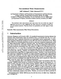
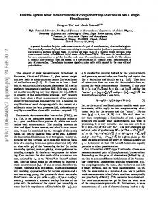
or a group of blindfolded observers, who can each only touch one part of the elephant, to construct an accurate representation of an elephant, the group must combine information about different parts of the elephant (FIG 1a). In quantum mechanics, to have a complete description of a quantum system, in particular, a complete knowledge of a quantum state, we must combine information about complementary aspects (FIG 1b). An ideal (strong) quantum measurement of a certain observable only gives the probabilities of obtaining the eigenvalues of the observable, and the statistical results of the measurements reflect the diagonal terms of the density matrix in the eigenbasis of the observable. Measurements of different (complementary) observables provide the diagonal terms of the density state for different bases. If we perform measurements for a sufficient number of bases, we can reconstruct the density state, which is the idea of state tomography. An important difference exists between the tomography of a quantum state and its classical counterpart, e.g., the description of an elephant by blindfolded observers. In this classical example, the description (of the elephant) by each man is not exclusive, and the different aspects of perception can be simply combined to produce an overall description of the elephant (FIG 1a). However, quantum physics forbids simultaneous knowledge of complementary observables because precise knowledge of a certain aspect necessarily implies uncertainty for the complementary aspects1. Therefore, one cannot simultaneously perform ideal measurements of complementary observables in quantum physics (FIG 2a). To determine the quantum state of a system, different measurement setups, each for a particular observable, are required. To determine the general state of a d-dimensional quantum system, at least d 1 1 different experimental setups are needed. Each setup must be devoted to the measurement of one of the complementary observables. An alternative state tomography approach is possible. Instead of obtaining maximum information of a particular observable by an ideal measurement, we can perform a weak measurement2. The state of the quantum system is only slightly changed during its weak interaction with the measuring device; therefore, weak measurements of a set of complementary observables can be performed simultaneously3 (FIG 2b). Thus, fewer experimental setups are needed for state tomography via weak measurements4. Weak measurements have been well described in the literature. Since they were first introduced by Aharonov, Albert and Vaidman2, weak measurements have been realised in experiments5–7, and have provided new insights into the study of paradoxes and fundamental problems in quantum theory8–12. Weak measurement has also been used as a practical tool for amplifying weak signals and signal-to-noise ratios13–20. Signal amplification via weak measurement usually involves a pre-selection and a post-selection that are nearly orthogonal, and the original formalism of weak measurement2,21 is not sufficient for the phenomena in this regime because it only retains the first-order terms of the interaction strength22–24. Extensions to the case of general pre-selection are given in (Refs. 25, 26). A framework that retains the high-order terms for general pre-selection and post-selection is given in (Ref. 27), and specific cases are further studied in (Refs. 28–30). A nonperturbative theory of weak pre- and
SCIENTIFIC REPORTS | 3 : 1193 | DOI: 10.1038/srep01193
1
www.nature.com/scientificreports
(a)
(a)
(b)
(b)
Figure 1 | (a) Compatible aspects are combined in classical physics, (b) while complementary aspects are combined in quantum physics.
post-selected measurements is given in (Ref. 31). The general results for the weak measurement of a pair of complementary observables are provided in (Ref. 20). Related concepts, such as the contextual values32 and modular values33, were also introduced. Weak measurements can also be used for state tomography. Lundeen et al.4 directly measured the wave function of a pure state by a weak measurement followed by a post-selection. The scheme was extended to the mixed state by sequential weak measurements of pairs or triple products of complementary observables34. The results of the weak measurements could also be interpreted in terms of the Kirkwood-Dirac representation via complex joint probabilities35,36. Reviews and additional references on weak measurements can be found in (Refs. 31, 37, 38). The results in (Ref. 4) demonstrate that the wave function of a pure state can be directly obtained from a single experimental setup, and that one can directly measure both the absolute values and the phases of the coefficients of a pure state in a certain basis. However, the scheme proposed in4 applies only to pure states, and it is not efficient because most of the data are discarded due to the post-selection. Here, we propose tomography schemes for both pure states and mixed states via weak measurements. Our schemes are more efficient because we do not discard any data. We also show that any (diagonal or offdiagonal) element of the density state can be directly determined as the average pointer shift in an appropriate weak measurement.
Results The idea. In the scheme proposed in (Ref. 4), the wave function to be measured is a continuous function of the position. The essence of the scheme is reviewed in finite dimensional Hilbert space as follows34,39. Suppose a quantum system with a d-dimensional Hilbert space is in an unknown state d {1 X yi jai i, ð1Þ jyi~ i~0
where the coefficients {yi} in a certain basis {jaiæ} need to be determined. The scheme for measuring the coefficients {yi} consists of a series of weak measurements of the observables Ai 5 jaiæ Æaij, each followed by the same postselection, i.e., a projection 1 X d{1 onto the final state jb0 i~ pffiffiffi i~0 jai i. The weak value of the d observable Ai is defined as 1 hb0 jai ihai jyi yi : Wi ~ ð2Þ ~ pffiffiffi hb0 jyi d hb 0 j y i Both the real and the imaginary parts of the weak value Wi have physical meanings and can be determined experimentally because they correspond to the average shifts of the pointer position and the momentum, respectively. From Eq. (2), we know that the weak values SCIENTIFIC REPORTS | 3 : 1193 | DOI: 10.1038/srep01193
Figure 2 | (a) A strong measurement only reveals a certain aspect of the quantum state, (b) while a weak measurement enables us to perceive (measure) incompatible aspects of the quantum state simultaneously.
Wi are directly proportional to the coefficients yi that we want to 1 can be determined by the measure and that the factor pffiffiffi d hb0 jyi normalisation condition (up to an unphysical overall phase of jyæ). Therefore, we obtain a direct measurement of the coefficients yi, thus a direct measurement of the wave function jyæ. The essential point in this scheme is the choice of the post-selected state jb0æ. Its overlap with each basis state . jaiæ has the same magnitude pffiffiffi and phase; therefore, the factor K~yi Wi ~ d hb0 jyi does not depend on i and can be determined by normalisation. Because the change of the system state due to a weak interaction with the pointer is negligible, the success probability of post-selection is given by P 5 jÆb0jyæj2. Therefore, only a fraction P of the data is retained, and the remainder is discarded due to the post-selection. When the dimension d is large, as in the case of a continuous wave function, the majority of the data is discarded. State tomography of a pure state. The part of the data that corresponds to the failure of the post-selection can be retained. We replace the final post-selection by a complete projective measurement onto the basis states {jbjæ}. The inner products bji 5 Æbjjaiæ are fixed when the two sets of the basis states are chosen. We organise the data according to the final state: if the final state is jbjæ, then the weak value of Ai 5 jaiæ Æaij is given by � � � � b bj jai hai jyi bj jai � ~� � yi ~ � ji � yi : ð3Þ Wji ~ � bj jy bj jy bj jy Therefore, for each fixed j, the weak values of different Ai give the relative ratios of the coefficients yi: � � � bj jy W � ð jÞ � � ~ ji bj jy : ð4Þ yi ~Wji bji bj jai Because Æbjjyæ does not depend on i, the coefficients yi are directly Wji proportional to , where the weak values Wji are read-outs directly bji from the experiments and the constants bji 5 Æbjjaiæ are fixed when ð jÞ the two sets of basis states are chosen. The super index (j) in yi denotes the coefficients yi that we obtain from the jth subset of the ð jÞ data. Ideally, yi should not depend on j; however, they may depend on j due to imperfections �� in �the � experiments. The � and � noise magnitude of the factor bj jy ~eiQj � bj jy � can be removed by normalisation: ffiffiffiffiffiffiffiffiffiffiffiffiffiffiffiffiffiffiffiffiffiffi �2 � ,v u u X ��Wji0 �� W ji ð jÞ t iQj ð5Þ yi ~e �: � � bji0 � bji i0 2
www.nature.com/scientificreports The phase factor Qj has no physical meaning because it corresponds to the overall phase of the pure state we are attempting to measure. This factor can be removed by a convention. For example, we require y0 . 0 (or the coefficient with the largest magnitude be positive). Using this approach, we retain all of the data and separate the data into d subsets according to the final states {jbjæ}. For the jth subset of the data that corresponds to the fixed final states jbjæ, we have an ð jÞ estimation of the coefficients yi from Eq. (4) or (5). A different subset of the data gives a different estimation for the set of coefficients {yi}. The differences between the estimations indicate the amount of error or noise in the experiment. When the basis {jbjæ} is mutually unbiased to the basis {jaiæ}, i.e., � � eiwji bji ~ bj jai ~ pffiffiffi, (5) can be simplified to ,sffiffiffiffiffiffiffiffiffiffiffiffiffiffiffiffiffiffiffiffiffi d X� � ð jÞ iQj {iwji �Wji0 �2 : ð6Þ Wji y ~e e i
i0
The original scheme proposed in4 corresponds to the case in which P jb0 i~ p1ffiffid d{1 i~0 jai i, and only the data corresponding to the successful post-selection of jb0æ are retained. Here, we retain all of the data, and each subset of the weak values corresponding to a fixed final state gives an estimation of the state to be measured. The probability of obtaining the final state jbjæ is given by jÆbjjyæj2 because the change of the system state during the weak interaction is negligible. When the state jyæ to be measured is almost orthogonal to a certain final state jbjæ, then the relative frequency to obtain the final state jbjæ in the post-selection is small. However, the corresponding weak value has a large magnitude, which could result in a large signal-to-noise ratio when the dominant noise is due to systematic error or imperfections. In the above scheme, weak measurements for a complete set of projective operators {Ai 5 jaiæÆaij} are needed. For the tomography of a pure-state wave function jyæ, weak measurements of a single observable instead of a set of observables are sufficient. This single observable can be chosen as follows (an alternative choice is presented in the Methods). We consider a pure state jQæ such that its overlap with each postselected state is nonzero, i.e., ÆbjjQæ ? 0 for each j. We perform a weak measurement of PQ 5 jQæÆQj. When the post-selected state is jbjæ, the weak value of PQ is defined as � � � � � bj �PQ jy bj jQ hQjyi � ~ � � : ð7Þ Wj ~ � bj jy bj jy Therefore,
� � � � bj jw hwjyi~gj hwjyi: ð8Þ bj jy ~ Wj � � bj jw is completely determined from the experimental Here, gj ~ Wj data and our choice because Wj is directly obtained from the experiment and both jQæ and {jbjæ} are fixed by our choice. From Eq. (8), we can reconstruct the state jyæ: X � � jyi~ ð9Þ Kgj �bj , j
where K is determined by the normalisation condition up to a phase.
Wji ~
tr
� � ��� �� �� � �� �bj bj � ðjai ihai jÞr bj jai ai jr�bj � � � � : �� �� � � ~ bj �r�bj tr �bj bj �r
ð10Þ
From Eq. (10), one can express the matrix elements of r either by the basis {jaiæ} � � � X bkj � � � � X bk �aj � � ai r aj ~ hbk jrjbk i Pk Wki ð11Þ Wki ~ bki hbk jai i k k or by the basis {jbjæ} X � � � � � � � �X hbi jak i b � ~Pj Wjk � Wjk ik , bi �r�bj ~ bj �r�bj bik b j j ak k k
ð12Þ
where the probability Pj 5 Æbjjrjbjæ corresponds to the frequency of obtaining the final state jbjæ in the experiment. The weak values Wji and the probabilities Pj are directly accessible from the experiment. The relationships in Eqs. (11) and (12) show that the matrix elements of the mixed state can be written as linear summations of the weak values that are directly accessible from the experiment. Partial state tomography. Using the idea of weak measurements, we can also selectively measure some of the matrix elements (diagonal and off-diagonal terms) of a state directly. This is especially useful when we are only interested in one or a few matrix elements of the state and we do not need to perform state tomography for the entire density matrix. Suppose we are interested in measuring a particular matrix element Æajrjbæ. We consider two different cases according to whether jaæ and jbæ are orthogonal. For the first case, suppose Æbjaæ ? 0. Here, we can simply perform a weak measurement of jaæÆaj, with a post-selection onto the state jbæ. The weak value is defined as W~
hbjaihajrjbi : hbjrjbi
ð13Þ
Thus, hajrjbi~
hbjrjbi W: hbjai
ð14Þ
W is the weak value, and Æbjrjbæ is the probability of success for postselection. Both values are directly obtained from the experiment. Æbjaæ is only a fixed factor. Therefore, Æajrjbæ is determined by Eq. (14). For the second case, suppose that Æbjaæ 5 0. We then perform a weak measurement of the observable C 5 jcæ Æcj with jci~ p1ffiffi2 ðjaizjbiÞ and a follow-up projective measurement onto a basis including both jaæ and jbæ as the basis states. We must only retain the data when the final state is either jaæ or jbæ. If the final state is jaæ, then the weak value of C is given by
� hajci hcjrjai 1 hbjrjai : ð15Þ W~ ~ 1z 2 hajrjai hajrjai If the final state is jbæ, then the weak value of C is given by
� hbjci hcjrjbi 1 hajrjbi 0 : W~ ~ 1z 2 hbjrjbi hbjrjbi
ð16Þ
We have State tomography of a mixed state. To this point, we have only considered tomography schemes for a pure state. If the state we like to measure is a general mixed state r, we also have a tomography scheme via weak measurements. For this case, we perform weak measurements for a complete set of projective operators Ai 5 jaiæÆaij, followed by a final projective measurement onto the basis {jbjæ}. For the initial state r and the final post-selected state jbjæ, the average shifts of the pointer position and the momentum in a weak measurement of Ai correspond to the real and imaginary parts of the weak value25,27 SCIENTIFIC REPORTS | 3 : 1193 | DOI: 10.1038/srep01193
hbjrjai~hajrjai ð2W{1Þ,
ð17Þ
hajrjbi~hbjrjbi ð2W 0 {1Þ:
ð18Þ
The post-selection probabilities Æajrjaæ and Æbjrjbæ and the weak values W and W9 are directly accessible from the experiment; therefore, we can determine the matrix element Æajrjbæ from either Eq. (17) or (18), which should agree with each other. Any discrepancies between them could be used as indicators of the noise and imperfections in the experiment. 3
www.nature.com/scientificreports Experimental scheme. Here, we discuss how our schemes can be realised experimentally. For the weak measurement of an observable A, the interaction between the measuring device and the system is generally modelled by a Hamiltonian H~gA6pdðt{t0 Þ, where p denotes the momentum of the pointer (measuring device). Because the interaction in a weak measurement does not change the state of the system significantly, weak measurements of several observables (whether they are commutative or not) can be performed simultaneously. The interaction of the simultaneous weak measurements of a set of observables {Ai} can be introduced by the Hamiltonian: X gi Ai 6pi dðt{t0 Þ: ð19Þ H~ i
Here, pi denotes the momentum of the ith pointer that is coupled to the observable Ai. {Ai} is an arbitrary set of observables of the system. They could be a set of commuting observables (for example, Ai 5 jaiæ Æaij) or even a set of complementary observables. Suppose the initial state of the system is rs, and the initial state of the pointers is rd 5 r1 fl r2 fl ???, where ri denotes the initial state of the ith pointer. Suppose the post-selection of the system is a projection Pj (for example, Pj 5 jbjæ Æbjj). Then the average position shift dqi and the average momentum shift dpi of the ith pointer are given by (see the derivation in the Methods) ð20Þ dqi ~gi ReWji dpi ~2gi ImWji ðDpi Þ2 :
ð21Þ
The weak value Wji of Ai, for a general initial state rs and a general postselection Pj , is given by20 � � Tr Pj Ai rs � � : ð22Þ Wji ~ Tr Pj rs The shifts of different pointers can be read out simultaneously, while either the position shift or the momentum shift is recorded at each time for each pointer. With the same Hamiltonian, we can obtain all of the weak values Wji. From these weak values, we can obtain all of the elements of the density matrix rs according to the state tomography strategy proposed in this article. Example of application. The state tomography schemes proposed here can also be used to detect a tiny parameter encoded in a quantum state. For example, to detect a tiny phase difference q picked up by two orthogonal states of a qubit (a photon) that passes through a certain medium (a birefringent crystal), we could 1 prepare a qubit in the initial state pffiffiffi ðj0izj1iÞ, and seek to 2 determine the tiny phase q encoded in the outgoing state � 1 � pffiffiffi j0izeiq j1i . To determine q, we can perform a weak 2 measurement of the observable j1æ Æ1j by introducing an interaction H~g j1ih1j6pdðt{t0 Þ between the qubit system and a measuring device and a follow-up post-selection of the qubit system 1 1 onto the state pffiffiffi ðj0i{j1iÞ. The weak value is W~1{i , and the q 2 1 average shift of the pointer momentum is given by dp~{2g ðDpÞ2 . q Although the phase q is small, the average shift of the pointer momentum is not necessarily small, and this has certain advantages over the quantum-entanglement based scheme in Ramsey interferometry40, which relies on the use of GHZ states of many qubits, which are an expensive resource.
Discussion In this article, we have proposed several schemes for state tomography via weak measurements. An advantage of our schemes is that we need to measure fewer observables compared with the standard SCIENTIFIC REPORTS | 3 : 1193 | DOI: 10.1038/srep01193
method of state tomography based on ideal measurements. For example, a simple standard state tomography requires ideal measurements in at least d 1 1 different bases; therefore, one needs to use at least d 1 1 different experimental setups. Here, our tomography strategy requires weak interaction in one basis ({jaiæ}) and post-selection in another basis ({jbjæ}), and the same interaction Hamiltonian is used for all data collection. Compared with the scheme in (Ref. 4), our strategy applies not only to pure states but also to mixed states. Our strategy is more efficient because we retain all of the data and thus reduces the number of experimental runs needed. Compared with the schemes in (Ref. 34) in which a density matrix is directly measured via sequential weak measurements of pairs or triple products of observables, our schemes are based on a single-time weak measurement followed by a strong complete projective measurement. Our interaction Hamiltonian in Eq. (19) is straightforward and differs significantly from those in the schemes of (Ref. 34). In the previous schemes4,34, the observables Ai 5 jaiæ Æaij require separate weak measurements at each time for a particular i. In our schemes, the set of observables {Ai} can be measured simultaneously via the interaction introduced by the simple Hamiltonian in Eq. (19). Interestingly, any matrix element of a density state is directly accessible from a suitable weak measurement. Ideal measurements give probabilities and expectation values, which are only linear combinations of the matrix elements of the density operator. Based on all of these facts, it is natural to draw the conclusion: what is and can be really measured in a general (ideal or weak) measurement is the density matrix (with all its elements), and only the density matrix!
Methods An alternative scheme for the tomography of a pure state via the weak measurement of a single observable. In the main text, we see that it is sufficient to perform a weak measurement of a single observable for the tomography of a pure-state wave function jyæ. This single observable could be chosen alternatively as follows. We introduce a single observable X A~ li jai ihai j, ð23Þ i
where the eigenvalues li are not degenerated, i.e., li ? lj if i ? j. We simply perform a weak measurement of the observable A and retain all of the data corresponding to different final states jbjæ. When the final state is jbjæ, the weak value of A is given by � � P � � P bj jAjy bj jai li hai jyi i bji li yi � ~ i � � ~ P ð24Þ Wj ~ � bj jy bj jy i bji yi From Eq. (24) we have
X bji li {Wj bji yi ~0:
ð25Þ
i
We define a unitary matrix b with the matrix elements given by the coefficients bji and introduce the diagonal matrices l 5 diag{l0, l1, ??? , ld21}, w 5 diag{w0, w1, ??? , wd21} and the vector ~ y~ðy0 ,y1 ,:::,yd{1 ÞT , where T denotes the transpose. Then, Eq. (25) can be written as ðbl{wbÞ~ y~0: ð26Þ With the notation M 5 bl 2 wb, we have M~ y~0. Thus, the state tomography in this case is to find the vector ~ y corresponding to the zero eigenvalue of M. The matrix M depends on w, which is determined by the weak values that are directly read out from the experiments. Due to noise and imperfections in the experiments, matrix M may not have a zero eigenvalue. Instead, multiplying M~ y~0 by M{ from the left, we have � { � ~ ð27Þ M M y~0: Therefore, the vector ~ y is the eigenvector in the kernel space of the non-negative matrix M{M. The vector ~ y is uniquely determined if M{M has a one-dimensional kernel space. It is not determined, and another set of measurements must be performed if M{M has a kernel space of more than one dimension. However, it is also possible that the matrix M{M determined from the experiment may not have a kernel space. In such a case, we choose the most likely one, i.e., we choose the vector ~ y as the eigenvector corresponding to the smallest eigenvalue of M{M. The value of the smallest eigenvalue of M{M indicates the amount of noise and imperfection in the experiment.
4
www.nature.com/scientificreports Derivation of the position shift and the momentum shift. Here, we derive the position shift and the momentum shift in (20) and (21), respectively. The time evolution Poperator corresponding to the interaction Hamiltonian in (19) is given by U~e{i i gi Ai 6pi . If the system is successfully post-selected by Pj , which occurs with a probability (to the first order of gi) of � �� � Pj ~Tr Pj 6I Urs 6rd U { ! ð28Þ X � � ~Tr Pj rs 1z2 gi ImWji hpi i i
the final (unnormalised) state of the pointers is given by (to the first order of gi) � �� � r0d ~Trs Pj 6I Urs 6rd U { ð29Þ !
X � � gi Wji pi rd {Wji� rd pi : ~Tr Pj rs rd {i
ð30Þ
i
Here, Trs (Tr) denotes the trace over the system (whole) Hilbert space. The average position shift of the ith pointer, conditional on the successful post-selction by Pj , is Tr ðqi p0d Þ
given by dqi ~ Trðr0d Þ gi gives
{hqi i. A straightforward calculation to the first order of
dqi ~gi ReWji zgi ImWji hfpi {hpi i, qi {hqi igi:
ð31Þ
When the initial states of the pointers are well-behaved states, such as Gaussian states, the second term on the right-hand side of (31) vanishes, and we immediately have (20). Similarly the average momentum shift of the�ith pointer, conditional on the � Tr pi r0d � 0 � {hpi i, which yields (21) to successful post-selection by Pj , is given by dpi ~ Tr rd the first order of gi. 1. Bohr, N. The quantum postulate and the recent developments of atomic theory. Naturwissenschaften 16, 245–257 (1928). 2. Aharonov, Y., Albert, D. Z. & Vaidman, L. How the result of a measurement of a component of the spin of a spin-1/2 particle can turn out to be 100. Phys. Rev. Lett. 60, 1351–1354 (1988). 3. Kocsis, S., et al. Observing the average trajectories of single photons in a two-slit interferometer. Science 332, 1170–1173 (2011). 4. Lundeen, J. S., Sutherland, B., Patel, A., Stewart, C. & Bamber, C. Direct measurement of the quantum wavefunction. Nature 474, 188–191 (2011). 5. Ritchie, N. W. M., Story, J. G. & Hulet, R. G. Realization of a measurement of a weak value. Phys. Rev. Lett. 66, 1107–1110 (1991). 6. Pryde, G. J., O’Brien, J. L., White, A. G., Ralph, T. C. & Wiseman, H. M. Measurement of quantum weak values of photon polarization. Phys. Rev. Lett. 94, 220405 (2005). 7. Hosten, O. & Kwiat, P. Observation of the spin Hall effect of light via weak measurements. Science 319, 787 (2008). 8. Aharonov, Y., Botero, A., Popescu, S., Reznik, B. & Tollaksen, J. Revisiting Hardy’s paradox: counterfactual statements, real measurements, entanglement and weak values. Phys. Lett. A 301, 130 (2002). 9. Wiseman, H. M. Grounding Bohmian mechanics in weak values and bayesianism. New J. Phys. 9, 165 (2007). 10. Mir, R., Lundeen, J. S., Mitchell, M. W., Steinberg, A. M., Garretson, J. L. & Wiseman, H. M. A double-slit ‘which way’ experiment on the complementarityuncertainty debate. New J. Phys. 9, 287 (2007). 11. Williams, N. S. & Jordan, A. N. Weak values and the Leggett-Garg inequality in solid-state qubits. Phys. Rev. Lett. 100, 026804 (2008). 12. Johansen, L. M. Weak Measurements with Arbitrary Probe States. Phys. Rev. Lett. 93, 120402 (2004). 13. Hosten, O. & Kwiat, P. Observation of the spin hall effect of light via weak measurements. Science 319, 787 (2008). 14. Dixon, P. B., Starling, D. J., Jordan, A. N. & Howell, J. C. Ultrasensitive beam deflection measurement via interferometric weak value amplification. Phys. Rev. Lett. 102, 173601 (2009). 15. Starling, D. J., Dixon, P. B., Jordan, A. N. & Howell, J. C. Optimizing the signal-tonoise ratio of a beam-deflection measurement with interferometric weak values. Phys. Rev. A 80, 041803(R) (2009).
SCIENTIFIC REPORTS | 3 : 1193 | DOI: 10.1038/srep01193
16. Brunner, N. & Simon, C. Measuring Small Longitudinal Phase Shifts: Weak Measurements or Standard Interferometry? Phys. Rev. Lett. 105, 010405 (2010). 17. Zilberberg, O., Romito, A. & Gefen, Y. Charge sensing amplification via weak values measurement. Phys. Rev. Lett. 106, 080405 (2011). 18. Feizpour, A., Xing, X. & Steinberg, A. M. Amplifying single-photon nonlinearity using weak measurements. Phys. Rev. Lett. 107, 133603 (2011). 19. Agarwal, G. S. & Pathak, P. K. Realization of quantum-mechanical weak values of observables using entangled photons. Phys. Rev. A 75, 032108 (2007). 20. Wu, S. & Z˙ukowski, M. Feasible optical weak measurements of complementary observables via a single Hamiltonian. Phys. Rev. Lett. 108, 080403 (2012). 21. Jozsa, R. Complex weak values in quantum measurement. Phys. Rev. A 76, 044103 (2007). 22. Duck, I. M., Stevenson, P. M. & Sudarshan, E. C. G. The sense in which a ’’weak measurement’’ of a spin-1/2 particle’s spin component yields a value 100. Phys. Rev. D 40, 2112 (1989). 23. Starling, D. J., Dixon, P. B., Williams, N. S., Jordan, A. N. & Howell, J. C. Continuous phase amplification with a Sagnac interferometer. Phys. Rev. A 82, 011802(R) (2010). 24. Geszti, T. Postselected weak measurement beyond the weak value. Phys. Rev. A 81, 044102 (2010). 25. Wiseman, H. M. Weak values, quantum trajectories, and the cavity-QED experiment on wave-particle correlation. Phys. Rev. A 65, 032111 (2002). 26. Wu, S. & Mølmer, K. Weak measurements with a qubit meter. Phys. Lett. A 374, 34 (2009). 27. Wu, S. & Li Y. Weak measurements beyond the Aharonov-Albert-Vaidman formalism. Phys. Rev. A 83, 052106 (2011). 28. Zhu, X. et al. Quantum measurements with preselection and postselection. Phys. Rev. A 84, 052111 (2011). 29. Nakamura, K., Nishizawa, A. & Fujimoto, M.-K. Evaluation of weak measurements to all orders. Phys. Rev. A 85, 012113 (2012). 30. Pang, S., Wu, S. & Chen, Z.-B. Weak measurement with orthogonal preselection and postselection. Phys. Rev. A 86, 022112 (2012). 31. Kofman, A. G., Ashhab, S. & Nori, F. Nonperturbative theory of weak pre- and post-selected measurements. Phys. Rep. 520, 43–133 (2012). 32. Dressel, J., Agarwal, S. & Jordan, A. N. Contextual values of observables in quantum measurements. Phys. Rev. Lett. 104, 240401 (2010). 33. Kedem, Y. & Vaidman, L. Modular values and weak values of quantum observables. Phys. Rev. Lett. 105, 230401 (2010). 34. Lundeen, J. S. & Bamber, C. Procedure for direct measurement of general quantum states using weak measurement. Phys. Rev. Lett. 108, 070402 (2012). 35. Johansen, L. M. Quantum theory of successive projective measurements. Phys. Rev. A 76, 012119 (2007). 36. Hofmann, H. F. Complex joint probabilities as expressions of reversible transformations in quantum mechanics. New J. Phys. 14, 043031 (2012). 37. Resch, K. J. Amplifying a tiny optical effect. Science 319, 733 (2008). 38. Aharonov, Y., Popescu, S. & Tollaksen, J. A time-symmetric formulation of quantum mechanics. Phys. Today 63, 27 (2010). 39. Salvail, J. Z. et al. Full characterisation of polarisation states of light via direct measurement. ArXiv:1206.2618 [quant-ph]. 40. Giovannetti, V., Lloyd, S. & Maccone, L. Advances in quantum metrology. Nature Photonics 5, 222–229 (2011).
Acknowledgements
The author likes to thank Marek Z˙ukowski for valuable discussions, and wishes to acknowledge support from the National Natural Science Foundation of China (Grants No. 11075148 and No. 11275181), the Chinese Academy of Sciences, and the National Fundamental Research Program.
Additional information Competing financial interests: The authors declare no competing financial interests. License: This work is licensed under a Creative Commons Attribution-NonCommercial-ShareALike 3.0 Unported License. To view a copy of this license, visit http://creativecommons.org/licenses/by-nc-sa/3.0/ How to cite this article: Wu, S. State tomography via weak measurements. Sci. Rep. 3, 1193; DOI:10.1038/srep01193 (2013).
5