Foundations and applications of weak quantum measurements

PHYSICAL REVIEW A 89, 052105 (2014)

Foundations and applications of weak quantum measurements Yakir Aharonov,1,2,3 Eliahu Cohen,1 and Avshalom C. Elitzur3,4 1

School of Physics and Astronomy, Tel Aviv University, Tel Aviv 69978, Israel Schmid College of Science, Chapman University, Orange, California 92866, USA 3 Iyar, The Israeli Institute for Advanced Research, Rehovot, Israel 4 The Solid State Institute, Technion, The Israel Institute of Technology, Haifa 32000, Israel (Received 3 July 2012; published 8 May 2014) 2

Weak quantum measurement (WM) is unique in measuring noncommuting operators and other peculiar, otherwise-undetectable phenomena predicted by the two-state-vector-formalism (TSVF). The aim of this article is threefold: (i) introducing the foundations of WM and TSVF, (ii) studying temporal peculiarities predicted by TSVF and manifested by WM, and (iii) presenting applications of WM to single particles. DOI: 10.1103/PhysRevA.89.052105

PACS number(s): 03.65.Ta, 03.65.Ca

I. INTRODUCTION

Superposition is the most intrinsic concept of quantum mechanics, an emblem of its uniqueness. The state of an unmeasured particle is not only unknown but indeterminate, co-sustaining mutually exclusive states. Equally crucial and ill-understood is “measurement” or “collapse” upon which one of these states is realized, inflicting uncertainty on conjugate variables. In view of these limitations, can there be any reason to make quantum measurement less precise? It is, surprisingly, weak measurement (WM) [1–16] that overcomes these limitations as well as many others [2–5,7]. Moreover, the two-state-vector formalism (TSVF), within which WM has been conceived, predicts several peculiar phenomena occurring between measurements, which only WM can reveal. Consider the question “What is the state of the particle between two measurements?” Obviously, measuring such a state would change it into a state upon measurement, rendering the question meaningless. Not so with WM: The state, almost without being disturbed, can be made known with great accuracy, moreover manifesting a host of new peculiarities [5]. Naturally, the TSVF claims are not unanimously accepted. Critics (e.g., [17]), while acknowledging its novelty, urge restating it in a simpler manner compatible with standard quantum theory. This article aims at meeting this challenge before proceeding to present some applications. Throughout this paper we will employ three methods for critical evaluation of WM’s strength: (1) Slicing. Meticulously recording individual (singleshot) WM outcomes, rather than a collective effect of many particles’ interaction with one device, enables grouping and summing up the outcomes according to later ordinary (“strong”) measurement outcomes, revealing an unequivocal weak-strong agreement. (2) Specific superposition. WM of a random ensemble of particles gives a normal distribution, which a skeptic may regard as a mere blend of strong measurement outcomes. We therefore employ a simple method of showing that WM is indeed performing the following feat: With an ensemble of particles sharing a very specific state, e.g., all split by a beamsplitter with some arbitrary transmission coefficient, WM can reveal this precise value (even unknown to the experimenter!) while leaving nearly all particles superposed [6]. 1050-2947/2014/89(5)/052105(10)

(3) Skeptical counterhypotheses. No discussion of TSVF, WM, and their far-reaching bearings can be complete without considering more prudent alternatives. Only after these are shown to be deficient is further exploration worthwhile. We will therefore give due hearing to such a generic alternative against every advance of our work. The outline of the article is as follows: Section II introduces the basics of TSVF and WM in a visualized manner. Section III, with a set of gedanken experiments, offers evidence for the most striking predictions derived from TSVF, namely the measurability of noncommuting variables during the same time interval, and the existence of two time-symmetric state vectors. Section IV presents an extension of WM for a single-particle case. II. FOUNDATIONS

As WM challenges our very concepts of quantum state and measurement, briefly revisiting the relevant formalism is in order. A. Formalism

First let measurement be put in formal terms. Then, weak measurement is attained by (i) loosening the coupling between measured and measuring objects (compared to the uncertainty of the measuring device), and (ii) summing up over many such measurements. 1. Loose coupling

Using von Neumann interaction Hamiltonian as in Ref. [5], a quantum measurement of the observable A is defined by the interaction Hint (t) = εg(t)APd ,

(1)

where the momentum Pd is canonically conjugated to Qd , representing the position of the pointer on the measuring device. The coupling g(t) differs from zero only at 0 t T and normalized according to T g(t)dt = 1, (2) 0

i.e., the measurement lasts no longer than T .

052105-1

©2014 American Physical Society

YAKIR AHARONOV, ELIAHU COHEN, AND AVSHALOM C. ELITZUR


In weak measurement, the coupling Hamiltonian of Eq. (1) is small in comparison to the standard deviation of the pointer, i.e., the measuring device is prepared in a symmetric quantum state with standard deviation σ ε and zero expectation. Without loss of generality we can refer to state | in the spatial representation (which serves as our measuring base) described by a Gaussian function (x) = exp(−x 2 /2σ 2 ).

(3)

The pointer movement in that case is connected to the weak value of the operator A defined by [1]: Aw =

ϕ|A|ψ , ϕ | ψ

(4)

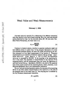
where |ψ is the initial (preparation) state of the measured system, and ϕ| is the final state into which it is projected. For a pre- and postselected ensemble described by the twostate ϕ||ψ, the time evolution of the total system (measured plus measuring system) is [5] ϕ| exp −i Hint dt |ψ| ≈ ϕ | ψ(1 − iεAw Pd )| (5) FIG. 1. Basic interferometers.

to first order in εAW , using = 1. This time evolution of Eq. (5) results in exp(−iεAw p)(x) = (x − εAw ),

2. Multiple outcomes

(6)

i.e., a shift proportional to the weak value. For example, when weakly measuring the spin z (described by the Pauli matrix σ z ) of an ensemble of spin-1/2 particles prepared in the √ |σx = +1 (“x-up”) direction, with coupling strength ε = λ/ N, the time evolution is determined by N √ W = exp −i Hint dt = exp iλ σnz Pd / N , (7) n=1

hence for a single measurement, the evolution of the spin state becomes entangled with the pointer of Eq. (3) (when σ = 1): √ 2 √ 2 1 [|σz = +1e−(x−λ/ N ) /2 + |σz = −1e−(x+λ/ N) /2 ] FN 1 λ2 2xλ 2 1−x − |σx = +1 + √ |σx = −1 , ≈ FN N N

It is on the ensemble level that weak measurement gains the desired precision, overcoming its inherent inaccuracy to the extent of even surpassing the limits of ordinary quantum measurement. By the large numbers law, if xi (the different measurement outcomes) are independent and identically distributed random variables with a finite second moment, a.s their average goes to their expectation value: x¯n → μ (that is, the average of the random variables tends almost surely to their expectation value). Furthermore, since the total variance (noise) is proportional to N , the relative error diminishes. It follows that N weak measurements, carried on an ensemble of particles that share the same value measured, amount to N strong measurements of that ensemble, while almost never giving rise to collapse. Hence, should the weak measurement be followed or preceded by a strong one, the latter would always confirm the result of the former result on the subensemble level.

(8) using the Taylor expansion of the exponent, where FN is a normalization factor. To complete the weak measurement, the pointer itself must be strongly measured. Then, the initial state of the particle |σx = +1 changes to |σx = −1 by only a small fraction ∼λ2 /N inversely proportional to the ensemble size. Statistically, this means that only ∼λ2 out of N states have changed. When λ is small enough, this number of “flipped” spins (changed from the initial “x-up” to “x-down”) is negligibly small compared to the size of the ensemble [18]. Moreover, if the coupling strength is ε = λ/N rather than √ ε = λ/ N , the weak measurement process will most likely end without a single flip.

B. Interferometry and the position-momentum tradeoff

Next let us put the above formulations in a physical context. For this purpose we briefly revisit the foundations of ordinary measurement before proceeding to WM. Consider the Mach-Zehnder Interferometer (MZI) [Fig. 1(a)]. It can be further simplified into its ancestor, the Michelson interferometer [19]. Let the two solid mirrors reflect the two split rays back to the beam-splitter (BS) [Fig. 1(b)]. As long as no measurement is made to find out which path the photon took after hitting the BS, then (provided that the difference between the half rays’ paths is an odd multiplication of half their wavelength) the photon always returns back to the source. Conversely, a “which path” measurement, even

052105-2

FOUNDATIONS AND APPLICATIONS OF WEAK QUANTUM . . .

of the interaction-free type [26] which does not absorb the photon, takes its toll: It indicates whether the photon was transmitted or reflected, but now, upon returning to the BS, it has a 50% probability to escape through the right-lower path [Fig. 1(d)]. Interference and “which-path” are thus related by the position-momentum uncertainty relation xp

2

(9)

and similarly for other pairs of noncommuting operators. In spin measurements, the BS is a Stern-Gerlach (SG) magnet. If no which-path measurement is carried out before the mirrors return the split wave function to the BS, the initial spin remains undisturbed. Here too, the two spin directions are related by an uncertainty relation analogous to Eq. (9). It is this uncertainty tradeoff, apparently insurmountable, that WM challenges. C. Measurement: None, ordinary, and weak

Based on the above setting, quantum measurement can be introduced at the fundamental level, its weak version following with equal simplicity. The position-momentum tradeoffs underlying quantum interference measurement are not trivial [21], so a few comments are in order. The simplest measurement can be performed by the reflecting mirrors. The splitting performed by the BS (preparation) is reversible. The reflecting mirrors, which instead of being fixed are attached to appropriate devices, complete the measuring process: One of them is pushed by the photon, thereby irreversibly recording its path.1 When, then, can measurement be considered weak? We can compromise either the separation or the recording stage. Most techniques take the former option, i.e., an incomplete separation between the two halves of the wave function [22,23]. In what follows, for measuring interference, we prefer modifying the second, recording stage. We therefore increase the momentum uncertainty of the mirror in comparison to the momentum exchanged with the photon, thereby making it harder to detect the photon. For such weakening, we must acknowledge a fact seldom mentioned in textbooks: Quantum uncertainty relations hold also for the measuring apparatus (see also [20]). Hence, with each mirror attached to appropriate detectors, the following holds.

PHYSICAL REVIEW A 89, 052105 (2014) 2. Measurement

Conversely, the mirror can be extremely light, such that its momentum is made 0 with high certainty. Any photon reflected by it imparts to it some of its momentum, disclosing its right or left position. However, in return for this momentum certainty of the mirror, its position becomes uncertain, thereby creating a difference between the two optical paths and ruining the interference [Fig. 1(d)]. 3. Weak measurement

Defining WM is now easy. Simply, give the mirror some intermediate mass: Large enough to blur photon-mirror momentum exchanges and allow interference, yet small enough for measuring some momentum transfer. This measurement outcome is, of course, very unreliable, as the momentum gain of the mirror is mainly a result of noise. Summing over many outcomes (Sec. II A 2), however, enables extracting the pure signal from the noise. D. Technical issues

Two technical questions remain to be addressed, as follows. 1. One or two path measurements?

In an ordinary which-path measurement, it does not matter whether we place one detector on one of the MZI paths or two on both. As the reading of one detector suffices, the other detector merely confirms it. Not so with WM: Placing two detectors amounts to performing two WMs, which may agree or disagree and thereby enhance or cancel one another. For this reason and for the next technical issue, we opt for one detector. 2. “Single shot” or collective outcomes?

The sufficiently-many N weak measurement outcomes can be obtained either (i) by the device interacting with all particles, accumulating their additive effects into the final outcome; or (ii) by the device being calibrated anew after each measurement, each outcome then individually recorded, to be summed up later under any desired grouping. In what follows we employ (ii). First, the former method inflicts an artifact in the form of slight entanglement between the collectively measured particles. Second, the “single shot” is vital for the slicing method, described next.

1. No measurement

When the mirror has a well-defined position, its momentum becomes proportionately uncertain. With a very heavy mirror, observing its motion due to the photon’s push is impossible. Hence no photon-mirror momentum transfer can be measured, nor can “which-path” information be gained [21]. Because its position is certain, the mirror does not change the optical path of the photon, giving rise to interference.

1

Notice the potential confusion to be avoided: we measure the photon’s position (right or left) by the momentum it conveys to the mirror.

E. Validation: Slicing reveals agreement between weak and strong measurements

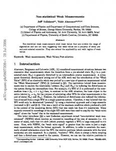
To what extent, then, is WM reliable? The test is straightforward. Let a sufficiently large number of individual particles undergo, one by one, a strong measurement followed by a weak one of the same variable. In our case this would be a which-path measurement of the photons within the interferometer. We thus obtain two lists of R (right) and L (left) outcomes, written precisely in parallel, to enable comparing the strong and weak outcomes of each individual particle (Fig. 2). Each single weak outcome is highly unreliable in itself, i.e., showing near 0 correlation with its strong counterpart. But now let us go to the list of strong values and draw a tortuous binary line that divides them, all Rs below the line and all Ls above. Next shift this

052105-3


FIG. 2. Weak measurements (gray detectors) followed or preceded by strong ones (black). The slicing procedure reveals the agreement between weak and strong measurements.

line to the parallel list of weak values. This list is thereby also divided. We now have two sublists of weak outcomes which, upon being separately summed up, give robust agreement with the corresponding sublists of strong R and L values: nR ≈ nL ≈ N/2 → n↑above ≈ n↓above + λ2 /2,n↓below ≈ n↑below + λ2 /2,

(10)

where nR / nL are respectively the number of right and left strong outcomes, and n↓above /n↓below are the numbers of weak “left” outcomes above and below the binary line. Similarly, n↑above /n↑below are the numbers of weak outcomes denoting “right,” above and below the binary line in Fig. 2. Here too, λ2 denotes the number of “flips” in each ensemble. Equalities in Eq. (10) are reached with larger and larger ensembles. How reliable is this result for each individual particle? Very much: Suppose you see only the list of weak values, and then obtain only the binary line which splits the unknown list of strong values. This line contains a large amount of information: “All outcomes above have one spin value and all others have the other.” But this is not enough. Once this line slices the weak list, and each sublist is separately summed over, you know with certainty the spin value of each individual particle. Upon being shown the strong list, your prediction is affirmed. F. Mixture counterhypothesis: Perhaps weak measurement is only an ensemble of measured and unmeasured states

As stated in the Introduction, skeptical alternatives must be considered against every unusual claim of TSVF. We therefore conclude this section with close consideration of such a rival account, fairly representative for its kind: Could WM be merely the combined effect of a few fully measured particles mixed within numerous others which remain totally unmeasured? Apparently, this counterhypothesis relies on


sound reasoning. In terms of Eq. (8) above, (1) the interference following weak position measurement is not complete: λ2 /2 photons still go to the right-hand “dark” side; (2) the slight deviation in the WM outcomes which later agrees with the strong outcomes distribution also differs from the expected random result by a mere λ2 particles; (3) perhaps, then, it is only those λ2 individual “flipped” photons that are responsible for the success of the weak measurement. It is the single shot method (Sec. II D) that enables a clear-cut falsification for this alternative: Simply remove the individual λ2 collapsed ones from the final summation. In practice this can be done for half of the collapses, where the photons escape through the right-hand side of the BS [Fig. 1(d)], while the other half return to the source like uncollapsed photons. We then expect a 50% reduction of the weak-strong agreement. This, however, is never observed. This proof will be presented also in Secs. III and IV within the relevant settings, but the conclusion is already straightforward: It is not the few collapsed photons traversing the MZI which give the observed positions while all others display interference. Rather, each photon undergoes a minute change so as to perform the overall feat. G. Gains and surprises: Measuring the “immeasurable”

So far, nothing seems to be surprising. The reliability of WM, as confirmed by strong measurement, is ensured by the large numbers law. A major surprise, however, is entailed by the fact that WM is equally affirmed by an earlier or a later strong measurement. This time symmetry brings the following three characteristics. 1. A state between two measurements

Consider a photon undergoing two measurements of noncommuting operators, e.g., polarization along the coplanar directions α and β at t1 and t2 respectively. By the uncertainty relations, repeating the α measurement at t3 is no more bound to repeat the t1 outcome. Now consider the intermediate time interval t1 < t < t2 . What is the state of the particle during this interval? It is obviously pointless to perform a measurement, because it would yield a state upon measurement! WM, however, enables turning the question into a physical one. Figure 3 gives the temporal order of the result: The intermediate state is equally affected by the past and future measurements. A detailed example of this feat is given in Sec. III. 2. Noncommuting variables of the same particle

The above effect entails an even more intriguing result: When the two strong measurements are made on noncommuting operators, then, for the intermediate states, these two operators can coexist with arbitrary precision. This will be shown in detail in Sec. III. 3. Exotic mass and momentum

With the uncertainty principle thus subtly outsmarted and ordinary temporal order strained, it is perhaps not surprising that these between-measurements states revealed by WM

052105-4



FIG. 4. (Color online) WM with a delayed-choice option. The transmission coefficient of the BS arbitrarily differrs from 50%. (a) Interference upon the split photon’s return to the BS proves that the photon has remained superposed despite the weak which-path measurement. (b) BS removed before the photon returns. The two lower detectors confirm the weak measurement outcome. FIG. 3. A particle undergoes three strong measurements (denoted by s) of noncommuting spin operators σ α and σ β . WM (denoted by w) shows that during the intervals t2 > t > t1 and t3 > t > t2 the state equally agrees, at the ensemble level, with the outcomes of the past and future strong measurements.

WM extends this reasoning to states inaccessible to standard quantum measurement. Hence its results, no matter how peculiar, are equally sound. III. PAST AND FUTURE EXERTING EQUAL EFFECTS

display other physical oddities. Particles with odd mass or momentum, at times being even negative, are predicted by TSVF and amenable to isolation and measurement by appropriate slicing. Such effects are demonstrated elsewhere [30]. H. Efficiency: Revealing specific superposition

As stated in the Introduction, the strength of WM strength can be demonstrated where the superposed state is a specific one. Let the BS transmission coefficient arbitrarily differ from the ordinary 0.5, say, 0.5 + η, where η is some small constant. We thus have N photons sharing a unique state: The position of √ each photon is√superposed yet very precise, namely |ψ = 0.5 + η|R + 0.5 − η|L. Suppose further that we do not know the value of η. Can we detect it? WM, over time, can. With N = 106 , λ = 3, for example, the error in estimating η would be only 10−5 which is very low. Apparently, this is merely the statistical distribution of the flips of the N photons to either side. Not so: Upon the photons’ returning to the BS, nearly all of them (N − λ2 ) continue back to their source, indicating interference. We can, conversely, remove the BS just after the upper mirror has performed WM and prior to the return of the photon to the BS [Fig. 4(b)]. With the slicing procedure (Sec. II E), we can show that the two lower detectors indeed confirm the weak “which path” measurement.

We proceed to the central assumption of TSVF: The physical values of a particle are equally determined by two state vectors, proceeding in both directions of time. The foundations of time-symmetric QM were laid in Ref. [24]. The probability for measuring the eigenvalue cj of an observable C, given the initial and final states |ψ(t ) and (t )|, respectively, can be described by the time-symmetric formula | (t )|cj cj |ψ(t )|2 P (cj ) =

. 2 i | (t )|cici|ψ(t )|

(11)

A. Double MZI: Past and future effects crossing over

From the Michelson and MZ interferometers we proceed to the double MZI (Fig. 5). An analogous experiment [4] has recently demonstrated both “which-path” and interference measurements within the double-slit experiment. A comprehensive discussion of this setting has been made in Ref. [16].

I. Summary: A deeper quantum realm

Standard quantum experiments rely on the basic premise of statistics: For an ensemble of particles sharing a certain value, measuring this value on the entire ensemble gives an expectation value that reflects the value of each individual particle. Quantum interference, for example, is always demonstrated on a multitude of particles, yet it proves that each individual particle has somehow passed through both slits. Similarly for the Bell-inequality violation: Once proved on an ensemble of pairs, it follows that each pair has been correlated due to a nonlocal effect.

FIG. 5. (Color online) A double MZI. The photon goes through the system unmeasured or measured while traversing MZI1 or MZI2 , respectively.

052105-5



The next surprise is brought by the final measurements. Having obtained and recorded each weak outcome separately, we now have the freedom to slice these outcomes into any subensembles as we choose. So, upon obtaining the N final L f and Rf outcomes, we divide the earlier MZI1 outcomes accordingly. Separately summing each subensemble, the total 50% L1 :50% R1 now gives its place to a slight but significant bias: #(L1 ) > #(R1 ) and #(L1 ) < #(R1 ) for each N/2. The initial and final measurements’ outcomes match with P → 1 as the ensemble grows. Indeed, the weak values of the projection operators πL1 ≡ |L1 L1 | and πR1 ≡ |R1 R1 | can be found according to Eq. (4):

FIG. 6. (Color online) Performing a sequence of strong-weakweak-strong measurements along a double MZI enables obtaining which-path information as well as interference. Photons detected at Lf or Rf belong to the subensembles passing through R1 or L1 respectively.

Let a photon pass through a system of two consecutive MZIs (Fig. 5). It traverses MZI1 superposed over L1 and R1 . Next it goes through MZI2 only on R2 (the interference exit of MZI1 ), finally exiting from MZI2 towards either Lf or Rf . If, however, the photon is measured along MZI1 , it takes either L1 or R1 . Consequently, it traverses MZI2 superposed on both sides. Finally, while interference has been disturbed upon the photon’s leaving MZI1 , it re-emerges in the two final measurements, whose Lf /Rf outcomes precisely match the earlier R1 /L1 ones. In other words, refraining from which-path measurement on MZI2 gives again the path traversed in MZI1 . These familiar uncertainty tradeoffs [Eq. (9)] take a new twist when the measurements are weak.

B. Validation by slicing

Let photons go one by one through the double MZI (Fig. 6), undergoing weak and strong measurements, underlined and boldfaced, respectively. A strong measurement is initially performed by the very emission of the photon from the bottom-left corner: It has definite momentum. Second comes a weak measurement (gray detector) of the photon’s path through MZI1 , followed by another weak measurement through MZI2 . Finally, a strong measurement is performed by the last two detectors on Lf and Rf . Have all measurements been strong, the uncertainty price would be as described above. Being weak, however, the measurement of MZI1 gives 50% L1 :50% R1 . Again, this does not indicate that each particle has taken either path: The next weak measurement, in MZI2 , gives 0% L2 :100% R2 , preserving the initial strong “right-up” momentum! Interference thus indicates that each photon has traversed both L1 and R1 , superposed.

πL1 w =

Rf |πL1 |L0 0.5 = = 1, Rf | L0 0.5

πR1 w =

Rf |πR1 |L0 0 = = 0, Rf | L0 0.5

(12)

in the case of perfect weak measurement. The affinity between conditional probability and time-symmetric interpretations was explained in Ref. [24] and indeed, these results can be achieved using basic probabilistic rules. The oddity of this result is obvious. The interference observed in MZI2 is supposed to amount to quantum erasure [25], namely, “forgetting” the which-path information of MZI1 . Yet the final measurement resurrects it. In TSVF terms, however, this result is very natural once we adopt its time-symmetric view: Just take the final measurement Lf /Rf outcome (postselection) as the initial condition (preselection) of the experiment and follow the consequences backwards. C. WM revealing an unknown transmission coefficient

This is the time for the second critical method mentioned in the Introduction, namely using WM to reveal a specific superposition unknown to the experimenter. Let the three BSs of our double MZI have transmission coefficients other than the ordinary 50%, and furthermore different from one another. Of many interesting combinations with potential technological applications [6], we take a simple one (Fig. 7). Let BS1 be α% transparent, BS2 β%, and BS3 the latter’s inverse. This choice enables undoing the second beam splitting, resurrecting the “which path” of MZI1 . In other words, both “which path” and interference are equally available. Finally, suppose that the experimenter is oblivious to all the BS coefficients. With WMs performed within MZI1 and MZI2 , plus strong measurement performed after BS3 , she can reveal all coefficients with any desired accuracy, while leaving nearly all photons superposed. Notice that this time the confirmation of the WM’s results is more obvious than slicing: the outcomes give straightforward correlation! D. Mixture counterhypothesis reconsidered

As in Sec. II, this is the time to consider again the skeptical account, to gain confidence in the results. Here too, the mixture counterhypothesis (Sec. II F) appears to be tempting by the interference being imperfect. Had the MZI1 which-path measurement been strong, L2 would have

052105-6



FIG. 8. A cyclic WM. IV. WM OF A SINGLE PARTICLE

We now turn to an extension of WM which sounds impossible by the very definition of this method: Can WM be performed on a single particle? A. Cyclic weak measurement

FIG. 7. (Color online) The double-MZI with two arbitrary transmission coefficients of its BSs. With the two weak and one final strong measurement it is possible to reconstruct all the unknown coefficients, even before slicing, demonstrating the method’s rigor.

been traversed by 50% photons. But it is weak, hence by Eq. (8) approximately λ2 /2 photons traverse L2 . These are the few photons that have been flipped by WM to this side. Indeed Tollaksen et al. [16] showed that, in order for WM to work, the L2 path must remain open. Blocking it (black square in Fig. 6) would ruin the expected resurrection. Is it possible, then, that these few flipped photons are responsible for the entire trick? To rule out this account, our slicing method derives from it the following prediction: Slicing the L2 outcomes according to accurate (AC) and inaccurate (IN) outcomes, i.e., L1 − Rf and R1 − L f matches and mismatches, should give λ2 , (13) 2N N − λ2 P (R1 |Lf ,I N) = , (14) 2N which can be straightforwardly predicted to fail. Suppose we use only 1/10 of the outcomes. Since λ can be small, e.g., 2 or 3, it is quite likely that the N /10 particles do not include these λ2 flipped photons. However, N /10 being still very large, we expect the same resurrection of the L1 /R1 outcomes within these subensembles too. P (R1 |Lf ,AC) =

E. Summary

TSVF presents two sets of results whose combination seems to be prohibited by orthodox quantum theory, namely observing interference while resurrecting the earlier whichpath information. This feat can be applied to any other pair of noncommuting operators. Not surprisingly, the soundest explanation for these effects is offered by the progenitor of WM, TSVF: A state between two consecutive measurements carries both their traces, past and future.

The strength of WM stems from the large numbers law: Over a sufficient multitude of particles, it enables obtaining almost full information about their quantum states without flipping almost any of them. Does this require measuring many particles or perhaps will many states of one particle do? Following (Fig. 8) is a variant which shows the answer to be in the affirmative. Let a source emit a photon to a Michelson interferometer and immediately be replaced by a bottom-left mirror detector. Next allow the photon to bounce back and forth between the lower and the upper mirror detectors, N times during period 2T, assuming negligible energy losses. Denoting WM as in Eq. (1), Hint = g(t)Pd |RR|/N,

(15)

where |RR|, the measured operator, projects the state on the right side, and Pd is canonically conjugated to Qd , representing the pointer position on the measuring device. The coupling g(t) is nonzero only for 0 t τ T and normalized according to τ g(t)dt = 1. (16) 0

The measurement device is described by the Gaussian wave function mentioned above. According to the Ehrenfest theorem, ˙ d = 1 [Qd ,H ] + ∂Qd = g(t)|RR| . Q (17) i ∂t N Integrating for every integer 1 m N yields (2m−1)T +τ/2 1 g(t)|RR| dt = . Qd = N 2N (2m−1)T −τ/2

(18)

Hence, after N steps we get Qd = 12 , the expected value. Thus, when N → ∞, the single-photon effect on the mirror at every interaction goes to zero, but the overall effect is measurable: A 1/2 unit of movement is transferred to each of the upper mirrors. The position of the photon is thereby measured, yet its superposition and resulting interference effect remain intact. Turning from the familiar WM performed on an ensemble to the present one performed on a single particle, the success

052105-7


FIG. 9. Cyclic strong-plus-weak measurements, represented by black and gray detectors, respectively, of unequal rays. Alice tries to find the different intensities of the split beams without “collapsing” her single photon.

probability (for a single particle) calculated in terms of fidelity [18], λ2 , (19) N2 becomes crucial. The reason is that after N WMs, we are left with a very high success probability: P (1) ≡ F = 1 −

P (N ) = (1 − λ2 /N 2 )N −−−−→ 1.

(20)

N→∞

Taking into account practical considerations, namely, prevalent reflection coefficient such as 1 − 10−7 in dielectric mirror with the appropriate optical coating, we find that N can reach 106 cycles with probability of 80%. Total success probability −6 2 would be ≈0.8e10 λ . B. Making the challenge harder: A single photon revealing an unknown superposition without collapsing it

As with the double-MZI (Sec. II L), following is a case where WM has a clear practical advantage over all other measurements. 1. Measuring n coefficients with one photon

Alice has a beam-splitter that splits the beam into more than two parts, n N where N is the sufficient number of weak measurement outcomes needed to be summed up for WM (Fig. 9). The n parts, summing up to 100%, have unequal intensities. Alice now asks Bob to measure all these varying intensities of her BS with maximal precision. Bob has only one photon, which, for sentimental reasons, he does not want to waste or even ruin its superposition. Can he do that? Four methods come into account: (A) Classical. Out of the question. You can measure the transmission coefficients of the beam splitters only with a macroscopic light beam of known initial intensity, which you later compare with those of the outgoing beams. All photons, in order to be counted, must be absorbed or impart some of their energy to the detector, changing their wavelength. (B) Quantum mechanical. Impossible again. You can use your photons one by one and count the number of those detected in each outgoing beam, but even if you use mirror detectors and the photons are not absorbed, their initial superposition is lost. (C) Weak measurement. Almost there. You can use photons such that they remain superposed even after the measurement, but they must be as many as possible.


FIG. 10. Making the strong measurement an interaction-free one ensures the recalibration of the initial position, preventing an additive “drift” of the wave function after each cycle.

(D) Cyclic weak measurement. Yes you can! For your single photon use the setting in Fig. 9, i.e., make the process cyclic: Place weak mirror detectors on the outgoing paths. Then release your photon from its source and immediately replace the source with another mirror detector. Now let your photon bounce back and forth within the system. This way, with strong and weak measurements cyclically alternating, you may find all transmission coefficients with any desired accuracy at a nonzero probability [see Eq. (16)]. 2. Measuring the wave function of a single particle

Making this measurement approximately continuous, i.e., performed on a wave function spread over space, amounts to measuring the entire wave function. A similar result, involving protective measurement of a single particle, has been presented by Aharonov and Vaidman [9]. They have used a process which resembles the one we described in Sec. II O, where instead of measuring weakly in the position representation, an adiabatic measurement has been performed in the energy representation. C. IFM comes for perfection

Single-particle WM is extremely vulnerable to collapse. As discussed in Refs. [8,18], the rate of interference disturbance after each measurement is λ2 /N , leading to the success probability of Eq. (16). It is possible however to minimize this risk by turning the strong measurement into an interaction-free type [26]. Within this setting, IFM performs in fact a quantum Zeno effect [27]: At each cycle it absorbs the small undesired part of the wave function “leaking” to the right-hand detector (Fig. 10), preventing the accumulation of such leaks. D. A single-particle double MZI

Finally we apply the single-photon version to the doubleMZI (Sec. II J). Let our single photon bounce back and forth through that system (Fig. 11). Let the bottom solid mirror act also as an ordinary detector in the sense of Sec. II C. In contrast, let the two top solid mirrors perform WMs. Here again, let the two BSs have arbitrary transmission coefficients as in Sec. L (Fig. 7). The rigor and reliability of all the WMs along this setting is immediately revealed by their correspondence with these BS coefficients. And here again, these pairs of measurements, manifesting interference due to momentum left undisturbed, do not disturb the position measurement taking place at the end of each cycle.

052105-8


PHYSICAL REVIEW A 89, 052105 (2014) F. Summary: Probing the nature of the wave function

Is the wave function a mere mathematical construct or a unique physical entity with objective existence? So far the wavelike properties of quantum phenomena have been demonstrated only post hoc, such as interference effects that only leave traces but can never be observed in real time. With WM, it seems that even this barrier is no longer insurmountable. V. CONCLUSIONS

FIG. 11. (Color online) A single-photon version of the double MZI experiment.

In this paper we reviewed the foundations of WM and TSVF and presented applications of both theory and technique. In practice, WM involves highly delicate technical issues. At the conceptual level, however, it should first be studied with the simplest settings possible, even gedanken, in order to fully appreciate its rigor and applicability. On this level, WM is easily shown to accurately indicate the state of a particle without paying the price normally exacted by the uncertainty principle, by measuring a particle during the time interval between two measurements. This method can be broadened so as to hold even for a single particle, thereby enabling measurements of states considered unreachable even for weak measurement as used so far. In all these cases the particle is shown to be equally affected by the past and the future measurements. This effect is bound to produce even more intriguing phenomena, to be presented in consecutive articles [30,31].

E. Mixture counterhypothesis reexamined

This time, dismissing the mixture counterhypothesis is even more straightforward: This hypothesis explains away the correlations as spontaneous flips. In the present case, should our single particle flip even once during the cyclic measurements, it has a 50% chance of failing to return to its original position. However, according to Eq. (16), success probability goes to 100%, i.e., no flips expected. No-cloning [28,29] and causality are not violated either, because of the limited precision of the weak measurement and the its long duration. See also [9].

It is a pleasure to thank P. Beniamini, S. Ben-Moshe, M. Dorfan, E. Friedman, R. Griffiths, D. Grossman, T. Landsberger, and M. Usher for helpful comments and discussions. We also thank several anonymous referees who helped us in clarifying several points and improve the structure of the paper. This work has been supported in part by Israel Science Foundation Grant No. 1125/10 and by the ICORE Excellence Center “Circle of Light.”

[1] Y. Aharonov, D. Z. Albert, and L. Vaidman, Phys. Rev. Lett. 60, 1351 (1988). [2] Y. Aharonov, A. Botero, S. Popescu, B. Reznik, and J. Tollaskan, Phys. Lett. A 301, 130 (2002). [3] Y. Aharonov, S. Popescu, D. Rohrlich, and L. Vaidman, Phys. Rev. A 48, 4084 (1993). [4] S. Kocsis, B. Braverman, S. Ravets, M. J. Stevens, R. P. Mirin, L. K. Shalm, and A. M. Steinberg, Science 332, 1170 (2011). [5] Y. Aharonov and D. Rohrlich, Quantum Paradoxes: Quantum Theory for the Perplexed (Wiley, Weinheim, 2005), Chaps. 16–18. [6] Quantum Retrocausation: Theory and Experiment, AIP Conf. Proc. No. 1408, edited by A. C. Elitzur, E. Cohen, and D. Sheehan (AIP, Melville, NY, 2011), pp. 120–131. [7] L. A. Rozema, A. Darabi, D. H. Mahler, A. Hayat, Y. Soudagar, and A. M. Steinberg, Phys. Rev. Lett. 109, 100404 (2012).

[8] L. Vaidman, Phys. Rev. A 87, 052104 (2013). [9] Y. Aharonov and L. Vaidman, Phys. Lett. A 178, 38 (1993). [10] M. R. Dennis and J. B. G¨otte, New J. Phys. 14, 073013 (2012). [11] M. R. Dennis and J. B. G¨otte, New J. Phys. 14, 073016 (2012). [12] G. J. Pryde, J. L. O’Brien, A. G. White, T. C. Ralph, and H. M. Wiseman, Phys. Rev. Lett. 94, 220405 (2005). [13] J. Story, N. Ritchie, and R. Hulet, Mod. Phys. Lett. B 5, 26 (1991). [14] P. Dixon, D. Starling, A. Jordan, and C. Howell, Phys. Rev. Lett. 102, 173601 (2009). [15] J. M. Knight and L. Vaidman, Phys. Lett. A 143, 357 (1990). [16] J. Tollaksen, Y. Aharonov, A. Casher, T. Kaufherr, and S. Nussinov, New J. Phys. 12, 013023 (2010). [17] N. D. Mermin, Phys. Today 64(10), 8 (2011). [18] A. Botero and B. Reznik, Phys. Rev. A 61, 050301(R) (2000).

ACKNOWLEDGMENTS

052105-9

YAKIR AHARONOV, ELIAHU COHEN, AND AVSHALOM C. ELITZUR [19] [20] [21] [22]

A. Michelson and E. Morley, Am. J. Sci. 1881, 120 (1881). B. Tamir and E. Cohen, QUANTA 2, 7 (2013). D. Ludwin and Y. Ben-Aryeh, Found. Phys. Lett. 14, 519 (2001). O. Zilberberg, R. A. D. J. Starling, G. A. Howland, C. J. Broadbent, J. C. Howell, and Y. Gefen, Phys. Rev. Lett. 110, 170405 (2013). [23] O. Zilberberg, A. Romito, and Y. Gefen, Phys. Scr., T 151, 014014 (2012). [24] Y. Aharonov, P. G. Bergman, and J. L. Lebowitz, Phys. Rev. 134, B1410 (1964).


[25] S. P. Walborn, M. O. Terra Cunha, S. Padua, and C. H. Monken, Phys. Rev. A 65, 033818 (2002). [26] A. C. Elitzur and L. Vaidman, Found. Phys. 23, 987 (1993). [27] E. C. G. Sudarshan and B. Misra, J. Math. Phys. 18, 756 (1977). [28] W. Zurek, Nature (London) 299, 802 (1982). [29] B. Tamir, E. Cohen, and A. Priel (unpublished). [30] Y. Aharonov, E. Cohen, D. Grossman, and A. C. Elitzur, EPJ Web Conf. 58, 01015 (2013). [31] Y. Aharonov, E. Cohen, and S. Ben-Moshe, EPJ Web Conf. 70, 00053 (2014).

052105-10