dag G = (V,E,λ) with λ : V −→ OA ∪ DA, satisfying the following properties: ... channel (e.g., A→B/C1); and rounded rectangles are data dependencies sched-.
Static fault-tolerant scheduling with “pseudo-topological” orderings C˘ at˘ alin Dima1 , Alain Girault2 , and Yves Sorel5 1 2
Universit´e Paris 12, 61 av du G´en´eral de Gaulle, 94010 Cr´eteil cedex, France INRIA Rhne-Alpes, 655 Av. de l’Europe, 38334 Saint-Ismier cedex, France 3 INRIA Rocquencourt, B.P.105 - 78153, Le Chesnay cedex, France Abstract. We give a graph-theoretical model for off-line fault-tolerant scheduling of dataflow algorithms onto multiprocessor architectures with distributed memory. Our framework allows the modeling of both processor and channel failures of the “fail silent” type (either transient or permanent), and failure masking is achieved by replicating operations and data communications. We show that, in general, the graph representing a fault-tolerant scheduling may have circuits; hence, the classical computation of starting/ending times, based upon a topological ordering, is inapplicable. We then provide a notion of “pseudo-topological ordering” that permits the computation of the starting/ending times even in the case of cyclic graphs. We also derive algorithms for computing the timeouts that are used for failure detection.
1
Introduction
Embedded systems are systems built for controlling physical hardware in a changing environment, and therefore are required to react to environmental stimuli within limited time. Therefore, the design of such systems requires thorough temporal analysis of the expected reactions. On the other hand, limitations on hardware reliability may require additional fault-tolerance design techniques and need of distributed architectures. The complexity of the design of such a system is usually coped with by decomposing the problem into subproblems. Usually, the fault-tolerance problem is the hardest to address: one solution is to handle it at the level of hardware; see [15, 14, 20], to cite only a few. This solution has been extensively studied in the past decade and is very useful for ensuring reliable data transmission, fail-signal, or fail-silent “processor blocks”, fault masking with “Byzantine” components and membership protocols. This approach is important as it hides a wealth of mechanisms for fault-tolerance from the software design; however, the types of failures it cannot handle need to be coped with at the design level. Another solution is to combine scheduling strategies with fault detection mechanisms [10, 11, 17, 16]. Such a solution is suited to system architectures in which communications are supposed to be reliable and communication costs are small. Moreover, dynamic schedulers require the existence of a reliable “master” component. All these induce some limitations on the use of such techniques in embedded systems.
A third solution is to introduce redundancy levels at the design time [19, 12, 2]. Fault masking strategies like primary/backup or triple modular redundancy (multiple if more than one failure has to be tolerated), voting components, or membership protocols are then designed for failure masking. The scheduling strategies take into account durations of communications, and therefore this approach seems to be the most appropriate to embedded systems in which limited computational power of part of the processors is combined with tight real-time constraints at the response level. The drawback of this solution is that it does not take into account channel failures. Taking into account both processor and channel failures is crucial in some highly critical and/or non-maintainable embedded systems, like vehicle control systems. Usually, this is achieved at the architecture level by triplicating the number of buses. But sometimes even triplication might not assure enough reliability, or just a more involved architecture is imposed, and then fail-silent channels must be taken into account during scheduling. On the other hand, in complex architectures, data transmission may involve routings, therefore specific fault-tolerant routing techniques [22, 4] may need to be applied. This problem is related to the so-called edge k-connectivity problem for graphs [3]. We propose a theoretical model for the problem of fault-tolerant static scheduling onto a distributed architecture. The basic idea is that a fault-tolerant scheduling will be the union of several non-fault tolerant schedulings, one for each possible failure patterns. Our model uses only basic notions from graph theory and a calculus with mins and maxs for computing execution times. We consider distributed architectures in which the memory is distributed too, in which we only abstract from the communication protocols onto each channel and the execution schemes on each “processor node”. Our model does not include any centralised control for detecting failures, or “membership protocol” for exchanging information about failure occurrence. On the other hand, we abstract from the “local fault-tolerance” mechanisms: we work with fail-silent components, an assumption which hides the mechanisms for achieving such behaviour4 . But this is fine, since our aim is not to provide a model for any fault-tolerant problem, but mainly for those in which fault-tolerance must be achieved for the whole system, hence requiring a global approach. We use timeouts in order to detect failures of data communications, but also in order to propagate failure information. The reason is that, in our replication technique, the replicas of the same data transmission do not necessarily have the same source, the same destination, or the same route. Therefore, some replicas of the same task may “starve” because their needed data do not arrive, and therefore they will not be able to send their data as well, propagating further this starvation to other tasks. This propagation is achieved with timeouts. The theoretical problem raised by this approach is that, due to the need of redundant routings, we may have to schedule non-acyclic graphs. In classical scheduling theory, cyclic graphs pose the problem of the existence of a scheduling. 4
Recent studies on modern processors have shown that fail-silence can be acheived at a reasonable cost [1].
2
Thanks to the construction principles of our fault-tolerant schedulings, this will not be the case in our framework, and this forms the core of our work and hence one of our original contributions. We solve this problem by introducing an original notion of pseudo-topological ordering, which models the “state-machine” arbitration mechanism between replicas of the same operation. We show that each scheduling with replication can be ordered pseudo-topologically, and therefore there exists a minimal execution of it. We also prove the existence of the minimal timeout mapping, which associates to each scheduled operation 1+ the latest time when it should start its execution, in any of the failure patterns that must be tolerated (all the execution times are expressed in time units, i.e., integers, hence the “1+”). These results are based upon two algorithms that can be seen as a basic technique for constructing a fault-tolerant scheduling. Though we have named it a “static scheduling” model, the behaviour of each node is quite dynamic as we construct “decision makers” on each component, capable of choosing at run time the sequence of operations to be done on that component. Moreover, both processor and channel failures are treated uniformly in our model, it is only at the implementation that they will differentiate. In this sense, we also comment on the restrictions that this uniform treatment imposes on the implementations. Finally, let us mention that this paper gives the theoretical framework for the heuristics studied in a previously published paper [5]. The paper is organised as follows: in the second section we define the problem of non-fault-tolerant scheduling of a set of tasks with precedence relations. The third section contains our graph-theoretic model of fault-tolerant scheduling, together with its principles of execution, formalised in the form of a min-max calculus of starting and ending times. The fourth section deals with the formalisation of the failure detection and propagation mechanisms. The core of this section is the computation of the minimal timeout mapping, used for failure detection. We end with some conclusions and future work.
2
Plain schedulings
This section is a brief review of some well-known results from scheduling theory, presented in a perhaps different form in order to be further generalised to faulttolerant scheduling. For reasons of convenience in defining and manipulating schedulings, and especially due to the possibility of having data dependencies routed through several channels, we chose to represent programs as bipartite dags (directed acyclic graphs): Definition 1. A task dag is a bipartite dag GA = (OA , DA , EA ). Nodes in OA are tasks and nodes in DA are data dependencies between tasks; e.g., (t1 , d1 ), (d1 , t2 ) ∈ EA , with t1 , t2 ∈ OA and d1 ∈ DA means that the task t1 , at the end of its execution, sends data to the task t2 , which waits for the reception of this data before starting its execution. 3
We will rely also on a notion of architecture graph, which is simply a bipartite undirected graph. Figure 1(left) represents an example of task dag. Here, OA = {A, B, C, D} and DA = {A→B, A→C, B→D, C→D}. Figure 1(right) represents an example of an architecture graph. Here, P1 , P2 , P3 and P4 are the processors and C1 and C2 are the communication links. B A→B
B→D
A→C
C→D
A
P2 D
P1
C
C1
C2
P4
P3
Fig. 1. Left: a task dag; Right: an architecture graph. In the field of data-flow scheduling, each operation is placed onto some processor and each data dependency onto some channel, hence yielding a kind of copy of the task dag GA , in which it is possible to have some data dependencies routed through several channels between their source and destination. Here we will call such a “placement” a plain scheduling and define it as follows: Definition 2. A plain scheduling of a task dag A = (OA , DA , EA ) is a labelled dag G = (V, E, λ) with λ : V −→ OA ∪ DA , satisfying the following properties: S1 For each v ∈ V such that λ(v) = a ∈ OA , for each b such that (b, a) ∈ EA , there exists v 0 ∈ V with λ(v 0 ) = b and (v 0 , v) ∈ E. That is, each scheduled operation must receive all its incoming data dependencies. S2 For each v ∈ V such that λ(v) = a ∈ DA , for each b such that (b, a) ∈ EA , there exists a sequence v1 , . . . , vk ∈ V with vk = v, λ(v1 ) = b, λ(v2 ) = . . . = λ(vk ) = a and (vi , vi+1 ) ∈ E for all 1 ≤ i ≤ k − 1. That is, data transmissions may be routed through several channels from their source to their destination. S3 For each a ∈ OA there exists exactly one v ∈ V such that λ(v) = a. That is, each operation is scheduled� exactly once. S4 For each a ∈ DA , the set v ∈ V | λ(v) = a forms a linear subgraph in G (and is nonempty by condition S2). That is, the routings of any given data dependency go directly from the source operation to the destination operation. Given an architecture graph GS = (P, C, ES ) and a mapping π : V −→ P ∪C, we say that the pair (G, π) is a plain scheduling onto GS if π satisfies the following condition: ∀v ∈ V, λ(v) ∈ OA =⇒ π(v) ∈ P Several clarifications and comments are needed concerning this definition. Firstly, note that in our definition, the architecture is “hidden” within the edges of the graph A. Moreover, the scheduling order on each processor is abstracted as edges (v, v 0 ) for which (λ(v), λ(v 0 )) 6∈ E and λ(v) 6= λ(v 0 ). Then observe that properties S1 and S2 show the difference between how operations and data dependencies are scheduled, hence the “bipartite dag” model 4
for task dags. Finally, note that there can be nodes v ∈ V such that λ(v) ∈ D A (that is, carrying a data dependency) and π(v) ∈ P (that is, scheduled onto some processor). These nodes model two things: reroutings between adjacent channels, and intra-processor transmissions of data. Figure 2 represents one plain scheduling of the task dag of Figure 1(left) onto the architecture graph of Figure 1(right). The notation “A/P4 ” means that π(A) = P4 ; ovals are operations scheduled onto some processor (e.g., A/P4 ); square rectangles are data dependencies scheduled onto some communication channel (e.g., A→B/C1 ); and rounded rectangles are data dependencies scheduled onto some processor for re-routing (e.g., A→B/P3 ). A plain scheduling, in our sense, is the result of some static scheduling algorithm. The restrictions on the placement of tasks or data dependencies, which guide the respective algorithm, are not visible here – we only have the result produced by such restrictions. A→B/C1
A→B/P3
A→B/C2
A/P4
B→D/C1
D/P3
C→D/C2
C/P4
B/P1
A→C/P4
Fig. 2. A plain scheduling of the task dag onto the architecture graph of Figure 1.
Once a plain scheduling is created and we know the execution time of each task and the duration of sending each data dependency onto its respective channel, we may compute the starting time for each of them by a least fix-point computation, based upon the following definition of an execution: An execution of a plain scheduling onto a distributed architecture is governed by the following three principles: P1 Each task is executed only after receiving all the data dependencies it needs. P2 Each data dependency is executed only after the task issuing it terminates. P3 Each operation (task or data-dependency) is executed only after all the operations that precede it on the same architecture component are finished. This worst-case computation is based on the knowledge of maximal duration of execution for each task, resp. data dependency, when it is scheduled onto some processor, resp. channel. The mapping d is constructed from this information in the straightforward manner. As an example, our scheduling in Figure 2 may give the minimal execution represented graphically in the figure at the left, where the duration of execution of each node in G is equal to the height of its corresponding box.
P1
C1
P3
C2
P4 0
A 2
A→B C
A→B B
C→D B→D
4 6 8
D 10 11
5
Formally, given a function d : V −→ , denoting the duration of executing each scheduled task and data dependency, we define two applications α, β : V −→ , called resp. the starting and the ending time, by the two following equations: � ∀v ∈ V, α(v) = max β(v 0 ) | (v 0 , v) ∈ E , β(v) = α(v) + d(v) (1)
The computation of α and β lies on the notion of topological ordering, which says that each dag G = (V, E) can be linearly ordered, such that each node has a bigger index than all of its predecessors in G. Placements that satisfy all the four requirements S1 to S4 of a plain scheduling, failing only on the requirement to be acyclic, cannot be executed: the system of equations (1) has no solution, which means that the schedule is deadlocked. It is important to note that the way such a plain scheduling (hence non faulttolerant) is obtained is outside the scope of our article. There exist numerous references on this problem, e.g. [21, 7, 9, 6, 13]. Before ending this section, let us remind the union operation on graphs: given two graphs G = (V, E) and G0 = (V 0 , E 0 ), their union is the graph G00 = (V ∪V 0 , E ∪E 0 ). Note that the two sets of nodes might not necessarily be disjoint, and in this case the nodes in the intersection V ∩ V 0 might be connected through edges that are in E or in E 0 .
3
Schedulings with replication
Our view of a static scheduling that tolerates several failure patterns is as a family of plain schedulings, one for each failure pattern which must be tolerated. This informal definition captures the simplest procedure one can design to obtain a fault tolerant scheduling: compute a plain scheduling for each failure pattern, then put all the plain schedulings together. There may be several ways to put together the plain schedulings, each one corresponding to a decision mechanism for switching between them in the presence of failures. For example, we may have a table giving the sequence of operations to be executed on each processor in the presence of each failure pattern. But this choice corresponds to a centralised failure detection mechanisms. And, as we are in a distributed environment and therefore the information on the failure pattern is quite sparse, we would rather have some distributed mechanisms for propagating failure pattern information, based on a local decision mechanism. To this end, we will assume that, in our family of plain schedulings, any two plain schedulings are not “contradictory” on the order they impose on each component in the architecture. That is, if in one plain scheduling G1 a task a precedes a task b on the processor p, and both tasks are scheduled onto p in another plain scheduling G2 , then in G2 these two tasks must be in the same order as on p. This assumption implies that, in the combination of all plain schedulings, each task or data dependency occurs at most once on each component in the architecture. This implies that we do not mask failures by rescheduling some operations and/or re-sending some data dependency. The propagation mechanism is then 6
the impossibility to receive some data dependency within a bounded amount of time – that is, a timeout mechanism on each processor. Consider, for example, the case of the task dag and the architecture graph given in Figure 1, and suppose that we want to tolerate either one failure for each channel, or one failure for each processor, with the exception of P3 (say, an actuator whose replication cannot be supported at scheduling). Suppose also that task D must always be on processor P3 . We will consider the plain scheduling of Figure 2(c) (it supports the failure of P2 ), and the plain schedulings of Figures 3(a) (for the failures of P1 and/or C1 ), and 3(b) (for the failures of P4 and/or C2 ). We will then combine these three plain schedulings into the scheduling with replication of Figure 3(c). B/P2
A→B/C2
A/P4 A→C/P4
C→D/C2
D/P3
C/P4
A/P1 A→B/P1
A→C/C1
A→B/P3
A→B/C1
B/P2
B/P1
B→D/C2
B→C/P2
C/P2 C→D/C1
A→C/P4 C→D/C2
C/P4
B→D/C2
A→C/C1 D/P3
C/P2 A→B/P1
A/P4
B→D/C1
(a) A/P1
A→B/C2
B→D/C1
(c)
B/P1 C→D/C1
D/P3
(b) Fig. 3. (a) A plain scheduling tolerating the failures of P1 and C1 . (b) A plain scheduling tolerating the failures of P4 and/or C2 . (c) The scheduling with replication resulting from the combination of the two plain schedulings (a), (b) and the one from Figure 2.
This approach hides the following theoretical problem: the graphs that model such fault-tolerant schedulings may contain circuits. Formally, the process of “putting together” several plain schedulings must be modelled as a union of graphs, due to the requirement that, on each processor, each operation is scheduled at most once. But unions of dags are not necessarily dags. An example is provided in Figure 4. We have a symmetric “diamond” architecture, given in Figure 4(a), on which we want to tolerate two failure patterns: {C1 , C5 } and {C2 , C4 }. We want to schedule the simple task dag of Figure 4(d), but with the constraint that A must be put on P1 and B must be put on P4 (say, because these processors are dedicated). The two failure patterns yield respectively the two reduced architectures of Figures 4(c) and (d). For both reduced architectures, we obtain respectively the plain schedulings of Figures 4(e) and (f ). When combined, we obtain the scheduling with replication of Figure 4(g). More precisely, on the middle channel C3 , the data dependency A→B may flow in both directions! However none of the circuits obtained in the union of graphs really come into play in a real execution – they are there only because such a scheduling models the set of all possible executions. 7
P1
P1
P2
C3 C4
P3 C5
P1 C2
C2
C1
P2
C3
A
C1 P3
P2
C3
P3
C4
A→B
C5
B P4
P4
P4
(a)
(b)
(c)
A/P1
A/P1
A→B/C2
A→B/C1
A→B/P3
A→B/P2
A→B/C3
A→B/C3
(d)
A/P1
A→B/P2
A→B/P3
A→B/C4
A→B/C5
B/P5
B/P5
(e)
(f )
A→B/C1
A→B/P2
A→B/C2
A→B/C3
A→B/C4
A→B/P3
A→B/C5
B/P5
(g)
Fig. 4. (a) An architecture graph. (b − c) The two reduced architectures corresponding to the failure patterns {C1 , C5 } and {C2 , C4 }. (d) The task dag to be scheduled. (e − f ) The two plain schedulings of (d) onto (b) and (c) respectively. (g) The union of (e) and (f ), which is not a dag!
The sequel of this section is dedicated to showing that the existence of circuits is not harmful when computing the execution of a scheduling with replication. We start with the formalisation of the notion of scheduling with replication. Definition 3. A scheduling with replication of a task dag A = (OA , DA , EA ) is a labelled dag G = (V, E, λ), with λ : V −→ OA ∪ DA satisfying the properties S1 and S2 of Definition 2, and the following additional property: S5 For each circuit v1 , . . . , vk , vk+1 = v1 of G, there exists d ∈ DA s.t. for all 1 ≤ i ≤ k, λ(vi ) = d. That is, the only allowed circuits in G are those labelled with the same symbol, which must be in DA . Since in schedulings with replication some operations might occur on several processors and some data dependencies might be routed through different paths to the same destination, the principles of execution stated in the previous section need to be relaxed. It is especially the first and the second principles that need to be restated as follows: An execution of a plain scheduling onto a distributed architecture is governed by the following three principles: P1’ Each task can be executed only after it has received at least one copy of each data dependency it needs. P2’ Each data dependency can be transmitted only after one of the replicas of the tasks which may issue it has finished its execution, and hence has produced the corresponding data. P3’ Same as principle P3. 8
We use a mapping d : V −→ , which denotes the duration of executing each node of the task dag (resp. from OA or DA ) onto each component of the architecture (resp. processor or communication link). We accept that some of the nodes may have zero duration of execution: it is the case with intra-processor data transmission; sometimes, even routings of some data dependencies between two adjacent channels may be considered as taking zero time. However we will consider that each complete routing of data through one or more channels takes at most one time unit. We will also impose a technical restriction on mappings d: for each circuit in G, if we sum up all the durations of nodes in the circuit, we get a strictly positive integer. This technical requirement will be essential in the proof of the existence of the minimal timeout mapping in the next section. Mappings d : V −→ satisfying this requirement will be called duration constraints. Definition 4. An execution of a scheduling G = (V, E, λ), with duration constraints d : V −→ , is a pair of functions f = (α, β), with α, β : V −→ , respectively called starting time and ending time, and defined as follows: 1. Any task must start after it has received the first copy of each needed data dependencies: for each a ∈ OA and v ∈ V with (a, λ(v)) ∈ EA , � α(v) ≥ min β(v 0 ) | λ(v 0 ) = a, (v 0 , v) ∈ E 2. Any data dependency starts after the termination of at least one of the tasks issuing it: for each a ∈ DA and v ∈ V with (a, λ(v)) ∈ EA , � α(v) ≥ min β(v 0 ) | (v 0 , v) ∈ E, λ(v 0 ) = λ(v) or λ(v 0 ) = a
3. Any task or data-dependency starts after the termination of all operations preceding it on the same architecture component: for each v, v 0 ∈ V with (v 0 , v) ∈ E and (λ(v 0 ), λ(v)) 6∈ EA , α(v) ≥ β(v 0 ) 4. The ending time of any given task or data-dependency is equal to its starting time plus its duration: for each v ∈ V , β(v) = α(v) + d(v). Executions can be compared componentwise, i.e., given two executions f 1 = (α1 , β1 ) and f2 = (α2 , β2 ), we put f1 ≤ f2 if, for each node v ∈ V , α1 (v) ≤ α2 (v) and β1 (v) ≤ β2 (v). We may then prove that the set of executions associated to a scheduling with replication forms a complete lattice w.r.t. this order, that is, an infimum and a supremum exists for any set of executions. Definition 4 is in fact a fixpoint definition in the lattice of executions. But we have not yet showed that this lattice is nonempty – fact which would imply that there exists a least element in it, which will be called the minimal execution. For plain schedulings, the existence of an execution is a corollary of the acyclicity of the graph G. As schedulings with replication may have cycles, we need to identify a weaker property that assures the existence of executions. The searched-for property is the following: Definition 5. A pseudo-topological ordering of a scheduling G = (V, E, λ) is a bijection φ : V −→ [1 . . . n] (where n = card (V )), such that for all v ∈ V , the following properties hold: 9
1. If λ(v) ∈ OA , then for each d ∈ DA for which (d, λ(v)) ∈ EA , there exists v 0 ∈ V such that λ(v 0 ) = d, (v 0 , v) ∈ E, and φ(v 0 ) < φ(v). 2. If λ(v) ∈ DA , then there exists v 0 ∈ V with (v 0 , v) ∈ E and φ(v 0 ) < φ(v), such that either λ(v 0 ) = λ(v) or (λ(v 0 ), λ(v)) ∈ EA . 3. For each v 0 ∈ V , if (v 0 , v) ∈ E, (λ(v 0 ), λ(v)) 6∈ EA , and λ(v 0 ) 6= λ(v), then φ(v 0 ) < φ(v). Lemma 1. Any scheduling G = (V, E, λ) has a pseudo-topological ordering . The proof of this lemma is constructive: we consider the following algorithm, whose entry is a scheduling G = (V, E, λ) of a graph A = (OA , DA , EA ) and whose output is a bijection φn : V −→ [1 . . . n] which represents a pseudotopological ordering of G: Algorithm 1 Pseudo-topological ordering 1 2 3 4
5 6 7 8 9
begin k := 1; X0 := ∅; while k ≤ n do Choose some node w ∈ V such that: ✤ For all w00 ∈ V such that (w 00 , w) ∈ E, λ(w00 ) 6= λ(w), and (λ(w00 ), λ(w)) 6∈ EA , λ(w00 ) 6= λ(w), we have w 00 ∈ Xk−1 ; ✤ If λ(w) ∈ DA , then ∃ w0 ∈ Xk−1 ∩ V with either λ(w 0 ) = λ(w) or (λ(w0 ), λ(w)) ∈ EA and such that (w 0 , w) ∈ E; ✤ If λ(w) ∈ OA , then ∀ b ∈ DA with (b, λ(w)) ∈ EA , ∃ w0 ∈ Xk−1 such that λ(w 0 ) = b and (w 0 , w) ∈ E; Xk := Xk−1 ∪ {w}; φ(k) := w; k := k + 1; end while end
Claim. The choice step at line 4 can be applied for any k ≤ card (V ). This claim can be proved by contradiction, since the impossibility to make the choice step in the algorithm would imply the existence of a circuit in the graph, whose nodes would be labeled with different symbols from OA ∪ DA , in contradiction with requirement S5. It follows that the algorithm terminates, that is, Xn = V . Therefore, the application φ : V −→ [1 . . . n] defined by φ(v) = k iff v is the node chosen at the k-th step, is a pseudo-topological order on V . This fact proves Lemma 1. Theorem 1. The set of executions associated to any scheduling G = (V, E, λ) is nonempty. Proof. First, we use our Algorithm 1 to construct a pseudo-topological ordering φ : V −→ [1 . . . n] of the scheduling G. Then, we construct an execution (αφ , β φ ) inductively as follows: We start with the pair of totally undefined partial functions αφ0 , β0φ : V → [1 . . . n]. That is, both αφ0 (v) and β0φ (v) are undefined for any node v ∈ V . Suppose then, by induction, that we have built the pair of partial functions φ φ ) associates to each → [1 . . . n] (resp. βk−1 ), such that αφk−1 : V (αφk−1 , βk−1 10
vertex v ∈ V with φ(v) ≤ k − 1 the starting execution time (resp. the ending execution time). We then extend these partial functions to a new pair (αφk , βkφ ) with αφk , βkφ : V → [1 . . . n], by defining αφk (vk ) and βkφ (vk ) (where vk is the k-th node of the pseudo-topological order, i.e., φ(vk ) = k) as follows: 1. First, we compute the two following numbers: � φ (v 0 ) | (v 0 , vk ) ∈ E and (λ(v 0 ), λ(vk )) 6∈ EA , φ(v 0 ) < φ(vk ) x1 (vk ) = max βk−1 n � φ (v 0 ) | (v 0 , vk ) ∈ E, λ(v 0 ) = b | max min βk−1 o b ∈ DA , (b, λ(vk )) ∈ EA , φ(v 0 ) < φ(vk ) if λ(vk ) ∈ OA , x2 (vk ) = � φ 0 0 0 min βk−1 (v ) | (v , vk ) ∈ E, φ(v ) < φ(vk ) and either λ(v 0 ) = λ(vk ) or (λ(v 0 ), λ(vk )) ∈ EA if λ(vk ) ∈ DA Note that, by the assumption that φ is a pseudo-topological ordering, all the sets involved in the above computations are � nonempty. 2. We then take αφk (vk ) = max x1 (vk ), x2 (vk ) and βkφ (vk ) = αk (vk )+d(vk ). It is then routine to check that αn and βn are indeed executions.
t u
Corollary 1. There exists a minimal execution associated to any scheduling G = (V, E, λ). Proof. The minimal execution is defined as follows: for each v ∈ V , � αmin (v) = min αφn (v) | φ pseudo-topological ordering of G βmin (v) = αmin (v) + d(v).
The figure here on the right gives the minimal execution for the scheduling in Figure 4 (in the absence of failures). The duration constraints are given by the vertical dimension of each rectangle, while the arrows without any target indicate lost arbitration between replicas.
4
P1
C1
P2
P3
C2
t u
P4 0 A
A
2
A→B B
A→C A→B B→D
C
B C→D B→D
C
C→D
D
4 6 8 10
Schedulings with replication and failures
The fault detection mechanism described in Section 3 uses timeouts on the scheduled task and data communications. This section is concerned with the formalisation of this mechanism. Again, we will make use of the notion of pseudotopological ordering: it will help us in computing the timeouts. Note that computing the timeout of a scheduled operation as the max of the ending times of all the operations that precede it in the scheduling might not work, because of the possible existence of circular dependencies: this is the same problem emphasised in Section 2, and which required the introduction of the notion of pseudo-topological ordering. 11
A failure pattern in a scheduling G = (V, E, λ) is just a subset F ⊆ V of nodes. In general, we will consider a set of failure patterns F ⊆ P(V ). The result of removing a set F of nodes from a scheduling G = (V, E, λ) is simply a labelled graph GF = (VF , EF , λF ) with EF = E ∩ (VF × VF ) and λF = λ . VF GF might not be a scheduling – some nodes may fail to satisfy the requirements S1 or S2 of Definition 3. This models the situation in which some operation does not receive one or more data that it needs. We will then say that GF is a scheduling reduced by the failure pattern F . If this graph contains a scheduling, i.e., there exists a scheduling GF = (V F , E F , λF ) with V F ⊆ VF and λF = λF , then we say that G tolerates VF the failure pattern F . Note that if G tolerates a failure pattern F , then it tolerates any failure pattern F 0 ⊆ F . On the other hand, if G tolerates two failure patterns F1 and F2 , then in general it does not tolerate F1 ∪ F2 . Hence, what we give as failure patterns are maximal combination of faulty components. Graphs like GF cannot be “executed” using the principles given in Section 3 since some nodes may not receive all their data – we call such nodes as starving. Starving operations and data dependencies are not executed and, in order to prevent the system from being blocked, the component should try executing the next operation in its own scheduling. This is precisely how our obtained schedules mask the failures. Hence, components detect only a limited part of the “failure scenario”, namely the subgraph which leads to the starving node. We will formally say that even starving nodes are executed, but imposing that their duration of execution be zero. We will also require that, when an operation receives all its data (i.e., is not starving), it must be started before its timeout expires – just to avoid going into “philosophical” problems about the feasibility of several “instantaneous actions” in zero time: Definition 6. An execution of a scheduling reduced by a failure pattern GF = (VF , EF , λF ), with duration constraints d : VF −→ and timeout mapping θ : VF −→ is a tuple of functions f = (α, β, ε), with α, β : VF −→ (the starting, resp. ending times) and ε : VF −→ {0, 1} (the execution bit), having the following properties: 1. For each v ∈ VF , if we denote UvF = {β(v 0 ) | v 0 ∈ VF , (v 0 , v) ∈ EF , and (λ(v 0 ), λ(v)) 6∈ EA , λ(v 0 ) 6= λ(v)} then α(v) ≥ max UvF . 2. For each v ∈ VF such that λ(v) ∈ OA and for each a ∈ DA such that (a, λ(v)) ∈ EA , if we denote: F Tv,a = {β(v 0 ) | v 0 ∈ VF , λ(v 0 ) = a, (v 0 , v) ∈ EF , and ε(v 0 ) = 1} � F ) . then α(v) ≥ min θ(v), maxa∈DA (min Tv,a 3. For each v ∈ VF such that λ(v) ∈ DA , if we denote TvF = {β(v 0 ) | v 0 ∈ VF , ε(v 0 ) = 1 and either (λ(v 0 ), λ(v)) ∈ EA or λ(v 0 ) = λ(v)} � ( then α(v) ≥ min θ(v), min TvF . 1 if α(v) < θ(v) 4. For each v ∈ VF , β(v) = α(v) + d(v) · ε(v) where ε(v) = 0 otherwise 12
Using the notion of pseudo-topological ordering (with slight modifications), we may prove that, for each timeout mapping θ, the set of executions of GF is nonempty. Moreover, we may prove that the minimal execution of GF , denoted (αF , βF , εF ) exists and can be computed as the least fix point of the following system of equations (here, minimality refers only to the tuple (αF , βF )): 1. For each v ∈ VF such that �λ(v) ∈ OA and for each a ∈ DA such �that � F F (a, λ(v)) ∈ EA , αF (v) = max min θ(v), max �a∈DA (min Tv,a ) , max � Uv F � 0 F 2. For each v ∈ V with λ(v) ∈ DA , αF (v) = max min θ(v), min Tv , max Uv .
3. And for each v ∈ V , βF (v) = αF (v) + d(v) · εF (v), where εF (v) = 1 if αF (v) < θ(v), εF (v) = 0 otherwise. F , TvF , and UvF are the notations from Definition 6. Here Tv,a However, a bad choice of a timeout mapping may induce that some operations that may receive all their data be not executed, because the wait for the reception of the respective data is greater than the timeout. We will therefore call an execution correct if this situation does not occur, that is:
Definition 7. An execution (α, β, ε) of GF is correct provided that it satisfies F ) 6= ∞ then ε(v) = 1. the following property: for each v ∈ VF , if max (min Tv,a a∈DA
Then, the minimal timeout ensures that the minimal execution of the scheduling G = (V, E, λ) reduced by any of the failure patterns from F is correct. We will construct this minimal timeout by repeatedly computing the minimal execution of each GF in which non-starving nodes have an infinite timeout, whereas starving nodes share the same timeout for different failure patterns F . Our algorithm starts with a zero timeout for all nodes, θ0 (v) = 0. At each F step i and for each failure pattern F , we utilize the timeout mapping θ i defined F F by θi (v) = θi−1 (v) if v is starving, and θ i (v) = ∞ otherwise. We compute the minimal execution (αF , βF , εF ) induced by this timeout mapping, and then we compute θi (v) as the maximum of the starting times for v in each reduced graph GF in which v is non-starving. In the following we denote GF = (V F , E F , λF ) the maximal scheduling included in the graph GF , assumed to exist for all F ∈ F . Algorithm 2 Timeout mapping computation 1 2 3 4 5 6 7 8 9 10
begin forall v ∈ V do θ0 (v) := 0; i := 0; repeat i := i + 1; forall F ∈ F do θi−1 (v) F put θi (v) = ∞
if v 6∈ V F (i.e., v is starving) otherwise F
F F (αF i , βi , εi ) := the minimal execution induced by θ i ; end for forall v ∈ V do θi (v) := max{αF i (v) + 1 | v ∈ VF }. F ∈F
11 until θi = θi−1 12 end
13
Proposition 1. For each i ∈ , θi ≥ θi−1 . The proof runs by induction on i, using the fact that mins and maxs commute F with inequalities and that for each F ∈ F , θ 0 is the smallest timeout mapping for which θ(v) = ∞ for non-starving nodes v. Proposition 2. Algorithm 2 terminates, i.e., there exists i ∈
with θi = θi−1 .
Proof. Remind that a path in a graph is called simple ifP it has no loop. We call the weight of a path p = (v1 , . . . , vk ) the sum w(p) = 1≤i≤k d(vi ). For each v ∈ V , denote M (v) the max of the weights of all simple paths in G ending in v. We may prove by induction on i that βiF (v) ≤ M (v) for each v ∈ V , fact which would end our proof since the mapping M would then provide an upper bound for the increments on θi . To this end, denote p = (v1 , . . . , vk ) the path that ends in some node v = vk and that is defined by the property that βiF (vj ) = αF i (vj−1 ). Hence, p consists of nodes on a “critical path” that ends in v. Two cases may occur: either v1 has no predecessor in V or is a starving node, hence is “executed” (actually, skipped) when its timeout expires. No other case F F is possible since (αF i , βi , εi ) is a minimal execution. In the first case, the claim is trivially proved, since p is a path that does not contain any circuit (again by definition of an execution). In the second case, we will assume that v1 is the only starving node in p and, moreover, that there does not exist another non-starving node v 0 which leads us to the first case. We have that 0
F F F αF i (v2 ) = βi (v1 ) = αi (v1 ) = θi−1 (v1 ) = αi−1 (v1 ) + 1 for some failure pattern F 0 . Since we have considered that the duration of any F0 F node is greater than 1 time unit, we then have that αF i (v2 ) = βi (v1 ) ≤ βi−1 (v1 ). 0 F (v1 ) ≤ M (v1 ). Therefore, On the other hand, by the induction hypothesis, βi−1 F βiF (v) = βiF (v) − αF i (v2 ) + βi (v1 ) ≤ w(p) + M (v1 ) Observe now that we must have (λ(v1 ), λ(v2 )) 6∈ EA . This follows from the assumption that v1 is starving, v2 is non-starving, and there exists no other non-starving node v 0 with βiF (v 0 ) = αF i (v2 ). But then, the concatenation of any simple path that ends in v1 with p cannot have circuits by requirement S5 in the definition of schedulings with replication. This means that w(p)+M (v1 ) ≤ M (v), fact which ends our proof. t u
Proposition 3. The timeout mapping θi which is computed by the algorithm is correct for all failure patterns and is the minimal timeout mapping with this property. Proof. The correctness of the timeout mapping is ensured by the exit condition of the loop – we may only exit the loop when, for each node, the computed timeout θi (v) exceeds all the starting times in each failure pattern, and hence only starving nodes may reach their timeout. The second property follows by showing, by induction on i, that for each correct execution (α, β, ε) we have F (αF t u i , βi ) ≤ (α, β). 14
As an example, for the scheduling with replication given in Figure 3, the minimal timeout mapping is the following: θ(A/P1 ) = θ(A/P4 ) = 1
θ(C/P4 ) = θ(A→B/C2 ) = 3
θ(B/P1 ) = θ(B/P2 ) = θ(A→C/C2 ) = 4 θ(C/P2 ) = θ(C→D/C2 ) = 6
θ(A→B/C1 ) = 5 θ(B→D/C1 ) = θ(B→D/C2 ) = 7
θ(C→D/C1 ) = θ(D/P3 ) = 9
5
Conclusions
We have presented some results on the fundamentals of a theory of static faulttolerant scheduling. The main problem we have investigated is the presence of circuits in unions of plain schedulings. We have introduced a notion of scheduling with replication, which models the loading of a system which is supposed to tolerate a family of failure patterns. We have also introduced the notion of execution of such a scheduling, which models some natural principles concerning the arbitration between replicas. We have also provided the notions of pseudotopological ordering and of timeout mapping, which assure the existence and the correctness of minimal executions of a scheduling with replication. Our work is only on the theoretical side, and the complexity of the algorithms in our paper is rather important for a practical use. In fact, all the problems treated here are NP-complete problems [8]. But we think that this theoretical layout may help developing heuristics for special architectures and/or special types of task dags, as it has been done in [18], and eventually compare the static scheduling performances with other techniques of fault-tolerant scheduling which take into account both processor and channel failures. Another possible approach for the fault-tolerant scheduling problem, that can tolerate both processor and channel failures, can be the combination of the redundancy techniques for processor failures with the fault-tolerant routing techniques. However, this combination seems not to have been given attention up to now.
References 1. M. Baleani, A. Ferrari, L. Mangeruca, M. Peri, S. Pezzini, and A. SangiovanniVincentelli. Fault-tolerant platforms for automotive safety-critical applications. In International Conference on Compilers, Architectures and Synthesis for Embedded Systems, CASES’03, San Jose, USA, November 2003. ACM. 2. J. Bannister and K. Trivedi. Task allocation in fault-tolerant distributed systems. Acta Informatica, 20:261–281, 1983. 3. B. Bollobas. Modern Graph Theory. Graduate Texts in Mathematics. Springer Verlag, 1998. 4. A. Chowdhury, O. Frieder, E. Burger, D.A. Grossman, and K. Makki. Dynamic Routing System (DRS): Fault tolerance in network routing. Computer Networks, 31:89–99, 1999. 5. C. Dima, A. Girault, C. Lavarenne, and Y. Sorel. Off-line real-time fault-tolerant scheduling. In Proceedings of 9th Euromicro Workshop PDP’2001, pages 410–417. IEEE Computer Society Press, 2001.
15
6. G. Fohler and K. Ramamritham. Static scheduling of pipelined periodic tasks in distributed real-time systems. In Euromicro Workshop on Real-Time Systems, EWRTS’97, Toledo, Spain, June 1997. IEEE Computer Society Press. 7. M.R. Garey and D.S. Johnson. Complexity bounds for multiprocessor scheduling with resource constraints. SIAM J. Computing, 4(3):187–200, 1975. 8. M.R. Garey and D.S. Johnson. Computers and Intractability, a Guide to the Theory of NP-Completeness. W. H. Freeman Company, San Francisco, 1979. 9. A. Gerasoulis and T. Yang. A comparison of clustering heuristics for scheduling directed acyclic graphs on multiprocessors. Journal of Parallel and Distributed Computing, 16(4):276–291, December 1992. 10. S. Ghosh. Guaranteeing Fault-Tolerance through Scheduling in Real-Time Systems. Phd thesis, University of Pittsburgh, 1996. 11. S. Ghosh, R. Melhem, D. Moss´e, and J. Sansarma. Fault-tolerant, rate-monotonic scheduling. Real-Time Systems Journal, 15(2), 1998. 12. A. Girault, C. Lavarenne, M. Sighireanu, and Y. Sorel. An algorithm for automatically obtaining distributed and fault-tolerant static schedules. In International Conference on Dependable Systems and Networks, DSN’03, San-Francisco, USA, June 2003. IEEE. 13. T. Grandpierre, C. Lavarenne, and Y. Sorel. Optimized rapid prototyping for realtime embedded heterogeneous multiprocessors. In Proceedings of 7th International Workshop on Hardware/Software Co-Design, CODES’99, Rome, Italy, May 1999. 14. H. Kopetz. TTP/A - the fireworks protocol. Research Report 23, Institut f¨ ur Technische Informatik, Technische Universit¨ at Wien, Wien, Austria, 1994. 15. H. Kopetz, A. Damm, Ch. Koza, M. Mulazzani, W. Schwabl, Ch. Senft, and R. Zainlinger. Distributed fault-tolerant real-time systems: The MARS Approach. MICRO, 9:25–40, 1989. 16. Y. Oh and S.H. Son. Enhancing fault-tolerance in rate-monotonic scheduling. Real-Time Systems, 7:315–330, 1993. 17. Y. Oh and S.H. Son. Scheduling hard real-time tasks with tolerance of multiple processor failures. Technical Report CS–93–28, Unversity of Virginia, May 1993. 18. C. Pinello, L. Carloni, and A. Sangiovanni-Vincentelli. Fault-tolerant deployment of embedded software for cost-sensitive real-time feedback-control applications. In Design, Automation and Test in Europe, DATE’04, Paris, February 2004. IEEE. 19. K. Ramamritham. Allocation and scheduling of precedence-related periodic tasks. IEEE Trans. on Parallel and Distributed Systems, 6:412–420, 1995. 20. F.B. Schneider. Byzantine generals in action: Implementing fail-stop processors. ACM Transactions on Computer Systems, 2:145–154, 1984. 21. J.D. Ullman. Polynomial complete scheduling problems. In Fourth ACM Symposium on Operating System Principles, pages 96–101, New-York, USA, 1973. 22. L. Zakrevsky and M.G. Karpovsky. Fault tolerant message routing for multiprocessors. In J. Rolim, editor, Parallel and Distributed Processing, pages 714–731. Springer Verlag, 1998.
16