putationally more difficult target because it usually consists of a variety of processors. Our method consid- ers both computing and communication time to min-.
Static Load Balancing of Parallel PDE Solver for Distributed Computing Environment Shuichi Ichikawa and Shinji Yamashita Department of Knowledge-based Information Engineering, Toyohashi University of Technology Tempaku, Toyohashi, Aichi 441-8580, JAPAN Abstract This paper describes a static load balancing scheme for partial differential equation solvers in a distributed computing environment. Though there has been much research on static load balancing for uniform processors, a distributed computing environment is a computationally more difficult target because it usually consists of a variety of processors. Our method considers both computing and communication time to minimize the total execution time with automatic data partitioning and processor allocation. This problem is formulated as a combinatorial optimization and solved by the branch-and-bound method for up to 20–24 processors. This paper also presents approximation algorithms that give good allocation and partitioning in practical time. The quality of the approximation is quantitively evaluated in comparison to the optimal solution or theoretical lower bounds. Our method is general and applicable to a wide variety of parallel processing applications.
1
Introduction
NSL [1] [2] is a numerical simulation language system that automatically generates parallel simulation programs for multicomputers from a high level description of PDE (Partial Differential Equations). NSL adopts an explicit FDM (Finite Difference Method) based on a boundary-fitted coordinate system and multi-block method. Though there are many parallel processing systems for PDE (e.g. //ELLPACK [3], DISTRAN [4], DEQSOL [5]), only sub-optimal static load balancing has been implemented, because the combinatorial optimization problem involved is computationally difficult to solve [6] [7]. As NSL adopts both a boundary-fitted coordinate system and multi-block method, the optimization problem can be simplified and solved by the
branch-and-bound method in practical time with offthe-shelf computers [8] [9]. This method takes both computation and communication time into consideration, and finds the most adequate number of processors for execution, thus avoiding the use of excessive processors that results in unnecessary delay of execution. In previous research [8] [9], the target computer system was assumed to be a parallel computer consisting of uniform processing elements. This study deals with a more general parallel processing environment, which consists of non-uniform processing elements. This situation is very common in distributed processing environments. However, the optimization problem becomes far more difficult to solve, because non-uniformity of processors means greater numbers of free variables.
2 2.1
Model of Computation and Communication Parallel Execution Model
In NSL, a physical domain with a complex shape can be described by a set of mutually connected blocks (multi-block method). As each block can have curvilinear borders, NSL maps a physical block of various forms to a rectangular computational block (boundary-fitted coordinate system). Figure 1 shows a physical domain of 3 blocks, each of which is mapped to the corresponding computational domain. The dotted line in the figure indicates the connected border of a block. The solid line is the real border of the domain, where the corresponding boundary condition is imposed. These features enable users to set precise boundary conditions while gaining additional performance, because a rectangular computational domain implies
Proceedings ISCA 13th Int'l Conf. Parallel and Distributed Computing Systems (PDCS-2000), pp. 399-405 (2000)
1
Bs0
1 2
Hi
Bi
2
Bs1
3
Bs2 Bs3
Wi
3 Physical
Computational
Figure 1: Physical Domain and Computational Domain a regular array of data and computations that are favorable to vector/parallel operations. NSL generates parallel explicit FDM program for multicomputers. Each block is a 2-dimensional array of grid points, on which difference equations are calculated. Each calculation of the difference equations can be executed in parallel due to the nature of explicit FDM, followed by communications to exchange data across the connected borders. The parallel PDE solver in NSL invokes this set of operations iteratively. The purpose of this study is to minimize the total execution time of this parallel PDE solver by distributing mutually connected rectangular blocks among nonuniform processors, considering both computation and communication time to avoid the use of excessive processors.
2.2
Framework of Static Load Balancing
Let the number of blocks be m, and the number of processors be n. The relationship m � n is assumed in this paper (as in previous studies [8] [9]), because the boundary-fitted coordinate system generally helps to keep m small and we are usually interested in bigger n when discussing static load balancing. Load balancing under general conditions is left for future study. Under this assumption, we can formulate the problem in two stages. First, one must find the best allocation of n distinguishable processors to m distinguishable blocks to minimize the execution time. Thus, the best combination of processors must be chosen to minimize the total execution time, leaving some of them unused if necessary. The calculation time can be made shorter by using more processors, but the communication time would be longer if more processors are used. In other words, the best balance must be found between calculation and communication. This is particularly important in a distributed computing
Figure 2: Partitioning of a Block environment, because communication time tends to be dominant. This problem can be formulated as a combinatorial optimization problem that is difficult to compute [10]. Section 4 describes how this problem can be solved. To determine the best processor allocation, we have to know the best partitioning of a block to a given set of processors. Here, we decided that each processor should deal with only one subblock, which is a rectangular fragment of block. Figure 2 shows the block Bi split into four subblocks Bs0 , ..., Bs3 . This method is simple and straightforward, and is intuitively expected to suppress the emergence of communication to the possible extent. Section 3 describes how a block can be partitioned to the allocated processors according to this rule. A more elaborate partitioning scheme can improve the estimated execution time despite increasing communication, but such a method can cause congestion of the network, resulting in unexpected and unjustifiable delay of execution. Therefore, our conservative decision would be regarded as appropriate in most circumstances. One may consider a more aggressive method in the case of clusters tightly connected by a fast and dedicated network hardware, although this is strongly dependent on the particular implementation.
2.3
Evaluation Function
The evaluation function of this optimization problem is the execution time of each repetition of PDE solver. This execution time T is given by T
=
max Ti
Ti
=
T ai + T ci .
i
(i = 0, 1, ..., n − 1),
(1) (2)
Here, Ti is the execution time on the i-th processor (Pi ). As each processor only deals with one subblock, let the subblock of Pi be noted as Bsi . T ai is the calculation time of Bsi , and T ci is the corresponding communication time. Based on experimental results
3 δ
Bsi
hi δ
δ
wi
δ
Figure 3: Subblock
with the NSL system, T ai is modeled as a linear function of the number of grid points in Bsi , which is noted as Sai . Also, T ci is a linear function of the number of grid points that participate in communication, which is noted as Sci . Such linear models have been widely used in past studies, because linear models usually fit well to measurement results. However, we have to note that past studies focused on parallel computers, which usually have powerful inter-connects between processors. In distributed computing environments, networks tend to be relatively weak and communication time can be far from linear in some circumstances. We adopt a simple linear model in this paper, but a more detailed analysis will be required in future work. Figure 3 shows a subblock which has all its borders connected. This is the worst case for communication, so we show the upper bound of communication quantity here for simplicity. Then, T ai and T ci are given by Sai
=
hi wi ,
(3)
T ai Sci
= =
Ctai Sai + Dtai , 2δ(hi + wi + 2δ),
(4) (5)
T ci
=
Ctci Sci + Cni Dtci .
(6)
Ctai is the time to calculate a difference equation for one grid point on Pi . Clearly Ctai is dependent on the performance of the processor Pi . Dtai is also a machine-dependent constant, which represents the overhead of the calculation. The communication parameters Ctci and Dtci are also machine-dependent constants. Cni is the number of communication links, which is 8 in Figure 3, and 3 for Bs0 and 2 for Bs2 in Figure 2.
Partitioning
This section describes the methods to partition a block for a given set of non-uniform processors. For an example, see Figure 2. This partitioning is a kind of combinatorial optimization with geometrical constraints. All heights and widths of subblocks must be integers (integer constraints), and the original block must be reconstructed from its rectangular subblocks like a jigsaw puzzle (geometrical constraints). Under these constraints, we have to find the best partitioning to minimize T described in Equation (1). This optimization problem is so difficult that two heuristic algorithms are presented and quantitively evaluated against a theoretical lower bound.
3.1
Heuristic Algorithm
The most intuitive approach to partitioning would be divide-and-conquer. First, processors are separated into two groups. Then the block is cut straight into two subblocks in accordance with the total performance of each group. Cutting along the shorter edge, the cross-section and consequent communication would be minimal. This process is recursively applied until each subblock corresponds to one processor. This simple technique, which is generally called recursive bisection (RB), has been widely used in scientific computations [11] [12]. Plain RB is not always good but many of its derivatives has been developed and examined [12] [13]. 3.1.1
Type 1
The first algorithm (type 1) is a plain recursive bisection method. We can think of (2n − 2) ways to split n processors into two groups at each level of RB. Intuitively, it seems good to split processor performance into halves, but this grouping itself is NP-hard [10] and still does not guarantee the best result because this is a combinatorial optimization. In this algorithm, the numbers of processors are split into halves at each level of RB. Then the block is split into two subblocks according to the ratio of accumulated processor performance in each group. This � n � ways at each level, but grouping still involves �n/2� we examine every possible grouping recursively and take the best result as the result of this approximation algorithm. 3.1.2
Type 2
The type 1 algorithm takes too much time and gives poor performance when many processors are available.
1 2 3 4
type1
Table 1: Common Parameter Dtai Ctci Dtci δ
type2
Parameters Value 10.0 0.2 0.1 1
Figure 4: Partitioning
Bsk
Bsi
Bsj
Bsk
Ti > Tk > Tj
Bsi
Table 2: Variety of Processors Ctai #proc. 0.0100 3 0.0050 3 2 0.0033 0.0025 1 1 0.0020
Bsj
Ti = Tj
Figure 5: Local load balancing One reason for this is that it makes the level of recursion so high that load balancing is too localized to get a good result. There are many ways to overcome this problem, including recursive p-section (p > 2). Here, we examine a simple variant of the type 1 algorithm. The second algorithm (type 2) is a modified recursive bisection. Only √at the first level, n processors are the partiequally split into � n� groups to accelerate √ tioning. The block is stripped into parallel � n� rectangles in accordance with the sum of processor performance. The type 1 algorithm is applied from the second level. All possible groupings are recursively examined as in the type 1 algorithm. Figure 4 displays how a block is partitioned for 10 non-uniform processors by the type 1 and the type 2 algorithm. The type of line shows the level of recursion in partitioning. 3.1.3
Local load balancing
Both type 1 and type 2 algorithms concern only the balance of calculation. In other words, they try to make the calculation time equal by managing the number of grid points for each processor. The result is that the faster processor tends to be a bottle-neck, because the faster processor takes more grid points, which usually means more communication time. Local load balancing is effective in such cases. After calculating the temporal partitioning by approximation algorithm, some of the grid points are transfered to level the loads between adjoining subblocks. In Fig-
ure 5, the load of Bsi can be transfered to Bsk or Bsj . As Tj is smaller than Tk , some of the grid points of Bsi are transfered to Bsj . This process is iteratively applied until no improvement is derived.
3.2
Estimation of Lower Bound
Though the optimal solution is the best measure for quantitative evaluation of heuristics, this partitioning problem seems too difficult to solve. Therefore, we adopt a lower bound of T , which is derived from the following relaxed problem. minimize subject to
T = maxi� Ti Hj Wj = i hi wi hi , wi ∈ R+
Let Hj and Wj be the height and the width of the block Bj , and hi and wi be the height and the width of a subblock Bsi which belongs to Bj . R+ means positive real numbers; that is, the integer constraints � are removed here. Also, the equation Hj Wj = i hi wi , which only requires the sum of the area of subblocks to be equal to the area of the original block, means that the geometrical constraint is removed. This relaxed problem is a kind of non-linear programming, but can be easily solved.
3.3
Evaluation of Partitioning Algorithms
Figure 6 shows the quality of approximation algorithms, which is normalized by the lower bound de-
T / T_lower
1.25 1.20
type1 type1 + local type2 type2 + local
1.15 1.10 1.05 1.00 0 10 20 30 40 50 60 70 80 90 100
T / T_lower
1.30
1.20 1.18 1.16 1.14 1.12 1.10 1.08 1.06 1.04 1.02 1.00 2e+5
n : Number of PE
(a) uniform processors
BLOCK
type1 type1 + local type2 type2 + local
B0
B1
PE0
PE1
PE4
PE5
B2
PE2
B3
PE3
PE1
B1
PE3
PE
PE0
PE0
PE2
PE1
B2
PE2
B 2e+6
2e+7
PE3
3
. . .
. .
PE
size
(a) approx1
(b) non-uniform processors
BLOCK B0
Figure 6: Evaluation of Partitioning Algorithms
PE0
B1 B2
rived from the relaxed problem. Note that all these results depend on simulation parameters, particularly on the ratio of calculation time to communication time. Here, we used the parameters shown in Table 1. Calculation latency and communication parameters are set equal for all processors here. Type 1 and Type 2 are the previously mentioned approximation algorithms. Additional local load balancing is applied in “+local” cases. Figure 6(a) shows the results with various numbers of processors where Ctai = 0.01 for all processors. The geometry of the block is set to W = 500 and H = 400. On the right side of this graph, communication becomes dominant over calculation. Regardless of the number of processors, type 2 shows a better performance than type 1. With type 2, local load balancing shows no effect, which it is natural because all processors have the same Ctai in this graph. Figure 6(b) displays the results with ten nonuniform processors, which are shown in Table 2. A block of a variety of grid points with a fixed aspect ratio (W : H = 5 : 4) is partitioned for these processors. Calculation is dominant on the right side of the graph, and communication is superior on the left side. As the approximation algorithms only consider calculation time in partitioning, the error is bigger on the left side. Type 1 and type 2 show similar results, but local load balancing works well for both algorithms, regardless of the ratio between calculation and communication.
4
BLOCK B0
Processor Allocation
This section outlines the method to find the best allocation of n distinguishable processors to m distinguishable blocks so as to minimize the execution time. For partitioning, the type 2 algorithm described in Section 3 is used with local load balancing.
(b) approx2 PE PE0
B1
PE1
B2
PE2
B3
PE3 . .
BLOCK
PE
PE1
PE1 PE2
B0
PE3
B3
. . .
PE4 . .
. . .
(c) approx3
Figure 7: Approximation Algorithms
4.1
Branch-and-Bound
Basically, every combination of processors must be examined to solve this kind of combinatorial optimization problem, but this is a difficult computation problem, as mentioned in Section 2.2. Therefore, some technique is required to reduce the search space. In this paper, a branch-and-bound method is adopted. Let T¯ be the execution time for the temporal feasible allocation. Given a set of processors for a subblock Bsi , the lower bound of Ti is easily derived by the relaxed problem mentioned in Section 3.2. If this lower bound is bigger than T¯ , the current allocation has no possibility of providing a more feasible solution. Therefore, the partitioning process for this allocation can be omitted and any groupings which include this allocation can be pruned to reduce search space.
4.2
Approximation Algorithms
A good approximation algorithm is important for practical use of the branch-and-bound method, because it gives the initial temporal feasible solution. The better the algorithm, the earlier the optimization process will finish because more search space is pruned. Figure 7 shows the three approximation algorithms examined in this paper. The following is a rough description of these algorithms 1 . The first algorithm (approx1) initially sorts blocks according to the number of grid points. Processors are 1 The
details are omitted due to lack of space.
1.40
Table 3: Simulation Parameters Parameter Value Parameter Value Cta0 0.0050 Dtai 10.0 0.0033 Ctci 0.2 Cta1 Cta2 0.0025 Dtci 0.1 Cta3 0.0020 δ 1
approx1 approx1 + local approx2 approx2 + local approx3 approx3 + local best effort
1.35
accuracy
1.30 1.25 1.20 1.15 1.10 1.05 1.00 4
8
12
16
20
n : Number of PE
(a) m = 4
also sorted by the order of performance. This algorithm then allocates processors in cyclic manner. The second (approx2) is the same as approx1 in sorting. It then allocates faster processors to bigger blocks in accordance with the share of total grid points and total performance. The third (approx3) is a variant of approx2. In approx2, the share is calculated first and used throughout the allocation process. On the other hand, approx3 updates the shares of blocks and the share of processors whenever a processor is allocated. This makes the allocation more precise.
4.3
Evaluation
The approximation algorithms are quantitively evaluated against the optimal grouping derived by the branch-and-bound method. The results of numerical simulations are shown in Figure 8. Approx1, approx2, and approx3 are the approximation algorithms described in Section 4.2. Local means the iterative local improvement described in Section 4.3. Best effort in the figure means the best result taken from approx1+local, approx2+local, and approx3+local. Simulation parameters are shown in Table 3. The number of processors are multiples of 4, and the processors of Cta0 , ..., Cta3 are equally included. The calculation latency parameters Dtai are all set to the same value, as are the communication parameters Ctci and Dtci . The height and the width of blocks are generated randomly as multiples of 10 between 100 and 1000. The result is the average of 20 trials.
approx1 approx1 + local approx2 approx2 + local approx3 approx3 + local best effort
1.35
accuracy
1.30 1.25 1.20 1.15 1.10 1.05 1.00 8
12 16 20 n : Number of PE
24
(b) m = 8
Iterative Improvement
The approximated allocation can sometimes be improved by exchanging and transferring processors between blocks. This improvement is done as follows. First, find the block Bi which includes the slowest subblock. Second, find the block Bj which includes the fastest subblock. Then, try to improve T by exchanging or transferring processors between Bi and Bj . This process is iteratively applied as long as T is improved.
4.4
1.40
Figure 8: Evaluation of Grouping Algorithms The error is slightly bigger when the a priori assumption m � n is not satisfied well (n ≤ 8 for m = 4 and n ≤ 12 for m = 8). However, when the condition m � n holds, the error is less than 5% for this parameter set by approx2+local and approx3+local. The average execution time of the approximation algorithm and the optimization algorithm is shown in Figure 9. All measurements are done on an Intel Pentium-II 400 MHz processor with 256 MB memory, FreeBSD 3.1R, and GNU C compiler (ver. 2.7). The “approx.” in Figure 9 means the sum of the execution time of approx1+local, approx2+local, and approx3+local. Approximation algorithms are reasonably fast, and the combinatorial optimization (“optimize”) is pragmatic for 20–24 processors.
5
Conclusion and Future Work
Static load balancing in a distributed computing environment is very challenging, because it involves many free variables and a quite vast search space. This study demonstrates that optimization problems can be solved for up to 20–24 processors in practical time by off-the-shelf computers. Our methods are based on a general combinatorial optimization technique, and hence applicable to a wide variety of applications if
time [sec]
1e+05 1e+04 1e+03 1e+02 1e+01 1e+00 1e-01 1e-02 1e-03 1e-04
approx.(m=4) optimize(m=4) approx.(m=8) optimize(m=8)
4
8
12
16
20
24
28
n : Number of PE
Figure 9: Execution Time calculation and communication time can be properly modeled. More study is required for partitioning. An exhaustive search to get the optimal partitioning is desirable, because the best partitioning would be a better measure than a lower bound to evaluate approximation algorithms. Also, simpler and more powerful approximation algorithms should be crafted. Currently, the grouping phase takes too much time because the branch-and-bound method is still not effective enough. More precise lower bounds and better approximation is required to drastically reduce search space.
Acknowledgments This work was partially supported by a Grant-inAid from the Ministry of Education, Science, Sports and Culture.
References [1] T. Kawai, S. Ichikawa, and T. Shimada, “NSL: High-Level Language for Parallel Numerical Simulation,” Proc. IASTED Int’l Conf. Modeling and Simulation (MS ’99), Acta Press, 1999, pp. 208– 213. [2] T. Kawai, S. Ichikawa, and T. Shimada, “NSL: High Level Language for Parallel Numerical Simulation,” Trans. Information Processing Society of Japan, vol. 38, no. 5, May 1997, pp. 1058–1067 (in Japanese). [3] E. N. Houstis and J. R. Rice, “Parallel ELLPACK: A Development and Problem Solving Environment for High Performance Computing Machines,” Programming Environments for HighLevel Scientific Problem Solving, P. W. Gaffney
and E. N. Houstis, Eds., Elsevier Science Publishers B. V., 1992, pp. 229–243. [4] K. Suzuki et al., “DISTRAN System for Parallel Computers,” Joint Symp. on Parallel Processing (JSPP ’91), Information Processing Society of Japan, 1991, pp. 301–308 (in Japanese). [5] T. Ohkouchi, C. Konno, and M. Igai, “High Level Numerical Simulation Language DEQSOL for Parallel Computers,” Trans. Information Processing Society of Japan, vol. 35, no. 6, June 1994, pp. 977–985 (in Japanese). [6] N. Chrisochoides, E. Houstis, and J. Rice, “Mapping Algorithms and Software Environment for Data Parallel PDE Iterative Solvers,” Special Issue of the J. Parallel and Distributed Computing on Data-Parallel Algorithms and Programming, vol. 21, no. 1, 1994, pp. 75–95. [7] N. Chrisochoides, N. Mansour, and G. Fox, “Comparison of Optimization Heuristics for the Data Distribution Problem,” J. Concurrency Practice and Experience, vol. 9, no. 5, 1997, pp. 319–344. [8] S. Ichikawa, T. Kawai, and T. Shimada, “Mathematical Programming Approach for Static Load Balancing of Parallel PDE Solver,” Proc. 16th IASTED Int’l Conf. Applied Informatics (AI ’98), Acta Press, 1998, pp. 112–114. [9] S. Ichikawa, T. Kawai, and T. Shimada, “Static Load Balancing for Parallel Numerical Simulation by Combinatorial Optimization,” Trans. Information Processing Society of Japan, vol. 39, no. 6, June 1998, pp. 1746–1756 (in Japanese). [10] M. R. Garey and D. S. Johnson, Computers and Intractability, Freeman, 1979. [11] G. C. Fox, “A Graphical Approach to Load Balancing and Sparse Matrix Vector Multiplication on the Hypercube,” Numerical Algorithms for Modern Parallel Computer Architectures, M. Schultz, Ed., Springer-Verlag, 1988, pp. 37–62. [12] G. C. Fox, R. D. Williams, and P. C. Messina, Parallel Computing Works!, Morgan Kaufmann, 1994, chapter 11. [13] H. D. Simon and S. Teng, “How Good is Recursive Bisection?,” SIAM J. Sci. Comput., vol. 18, no. 5, Sept. 1997, pp. 1436–1445.