Temperature Aware Load Balancing for Parallel Applications ...

Temperature Aware Load Balancing for Parallel Applications: Preliminary Work Osman Sarood, Abhishek Gupta, Laxmikant V. Kalé Department of Computer Science University of Illinois at Urbana-Champaign Urbana, IL 61801, USA {sarood1, gupta59, kale}@illinois.edu

Abstract—Increasing number of cores and clock speeds on a smaller chip area implies more heat dissipation and an ever increasing heat density. This increased heat, in turn, leads to higher cooling cost and occurrence of hot spots. Effective use of dynamic voltage and frequency scaling (DVFS) can help us alleviate this problem. But there is an associated execution time penalty which can get amplified in parallel applications. In high performance computing, applications are typically tightly coupled and even a single overloaded core can adversely affect the execution time of the entire application. This makes load balancing of utmost value. In this paper, we outline a temperature aware load balancing scheme, which uses DVFS to keep core temperatures below a user-defined threshold with minimum timing penalty. While doing so, it also reduces the possibility of hot spots. We apply our scheme to three parallel applications with different energy consumption profiles. Results from our technique show that we save up to 14% in execution time and 12% in machine energy consumption as compared to frequency scaling without using load balancing. We are also able to bound the average temperature of all the cores and reduce the temperature deviation amongst the cores by a factor of 3.

I. I NTRODUCTION Large data centers can cost millions of dollars with cooling needs incurring nearly half the total energy cost [1]. Recent reports show that, in 2006, data centers in US alone used 59 billion KWh of electricity, emitted 864 million tons of carbon dioxide and costed up to US $4.1 billion [2]. This represented 2% of USA’s total energy budget. Recent legislative efforts [3] and increasing cost of power now make it difficult for data center managers to overlook energy efficiency any longer. Increasing number of cores and clock speeds on a smaller chip area implies more heat dissipation and an ever increasing heat density. This is fast becoming a problem in high performance computing (HPC). This problem is further aggravated by the advent of multithreading. Most cores can now achieve a very high rate of utilization and hence end up dissipating a lot of heat. The increased power dissipation and thermal densities have made systems far more vulnerable to transient and permanent faults. Spatial temperature variances i.e. hot spots, affect the reliability, cooling costs and performance of the system. Hot spots accelerate failure mechanisms which can cause permanent device failures [4]. Even small differences in temperatures e.g. 10-15 ◦ C, can cause a 2X reduction in the mean time to failure [5]. In addition to hot spots, temperature gradients in time and space also determine the

device reliability [6]. The failure rate due to thermal cycling increases with an increase in the frequency and amplitude of the temperature cycles [5]. Thermal cycling can also cause increased plastic deformations of materials which can lead to permanent failures. Leakage power is a major constituent of power consumption. In feature sizes of below 65nm, leakage is expected to account for more than 50% of the overall power consumption [7]. This leakage consumption is dependent on device temperature with a positive feedback loop existing between leakage and temperature. This can cause dramatic increase in temperature which, unless controlled, can damage the circuit. In addition to large spatial temperature variation across nodes causing hot spots, another factor that can cause performance degradation and logic failures is the spatial temperature variation across the chip within a node. Increasing temperatures give rise to increasing local resistances which cause an increase in circuit delays and IR drop [8]. The observations mentioned above motivated us to adjust the frequencies of all the cores inside a chip so that we avoid such on chip temperature variations and minimize the possibility of hot spot formation. The problem of scheduling tasks in order to avoid hot spot formation in data centers has been looked at in great detail [9] [10]. Although these works also try to minimize the load imbalance, they do not suffer a huge penalty if a few nodes are overloaded. In HPC, however, applications are typically tightly coupled and even a single overloaded core can adversely affect the execution time of the entire application. This makes load balancing of utmost value. Hot spots are obviously a major source of energy wasted on cooling. Many data centers decrease the overall room temperature in order to cope with the hot spot [11] and therefore waste energy in cooling machines that are already at the desired temperature. Most energy related work in HPC has been done with the aim of reducing the energy consumed by the machine itself while ignoring the cost of cooling. Surveys also show that for every watt consumed by the machine, it takes 1 to 2 watts to cool it depending on the cooling efficiency of the system [12]. Our major goal is to avoid this energy waste caused by the hot spots by ensuring that the temperature for each core does not exceed a threshold. For this, we want to minimize the temperature variance across the cores. We accomplish this

by periodically measuring the temperature at each core and using dynamic voltage and frequency scaling (DVFS) to scale down the frequency of a core if and when it crosses a userdefined threshold. This, however, causes different cores to work at different speeds and hence leads to load imbalance. To deal with this, we apply a greedy load balancing algorithm. This algorithm assigns tasks by taking into account the core frequencies and the amount of work. Although there have been some studies addressing the issue of hot spots, there haven’t been many for HPC. Especially lacking are studies that show experimental results instead of simulated ones. The major contribution of our work is hot spot avoidance and temperature control demonstrated by experiments. In our work, we use an 8 core machine and a watt meter for making energy measurements. Although our scheme is equally applicable to most programming models, in this paper we have implemented it using Charm++ [13]. Another feature of our scheme is its ability to make load balancing decisions at runtime rather than requiring any pre runs to generate traces. The rest of this paper is organized as follows. In Section II, we provide an overview of the related work. Section III describes our algorithm. Next, we analyze the performance of our algorithm in Section IV. Section V outlines our conclusions and some directions for future work. II. R ELATED W ORK The importance of saving energy spent in cooling towards the overall power savings has been studied previously [9] [14] [15]. Scheduling tasks to avoid thermal hot spots in data centers has also been looked at before [10][16] [17] [18] [19]. Choi et al. [10] investigated the trade-offs between temporal and spatial hot spot mitigation schemes and thermal time constants, workload variations and microprocessor power distributions. Also, they examine the effect of OS-level temperature-aware scheduling to avoid hot spots. The idea of frequency scaling with temperature variation has also been explored earlier. Rajan et al. [20] discuss the effectiveness of system-throttling for temperature aware scheduling. They claim that under certain assumptions, system-throttling rules are the best one can achieve. One of their assumptions is that the tasks on different cores can not be moved from one core to another which may not be valid in HPC. Runtime load balancing techniques such as those discussed in Section III are central to the performance of parallel applications such as NAMD [21]. One such approach has been taken in [22]. Their scheduler considers the energy characteristics of individual tasks to move them from overheated cores to others. This differs from our approach as it does not consider parallel applications. Researchers have also explored OS-level techniques such as thermal-aware task scheduling to minimize hardware DTM (dynamic thermal management techniques such as frequency and voltage scaling) [23]. These techniques classify jobs into hot/cold jobs and schedule them so as to maintain temperature

under thermal threshold. Various scheduling algorithms such as random and prioritized scheduling have been explored. Approaches which are hybrid of software techniques such as OS-level task scheduling and hardware techniques such as frequency scaling have also been considered [24]. Load balancing mechanisms designed for non HPC data centers aim at distributing load as equally as possible. However, if any one of the servers is overloaded, it does not affect the entire system as badly as it would in the case of an HPC data center due to presence of synchronization primitives. Most of the work done for HPC data centers has focused on saving energy consumed by the system and has ignored cooling costs [25]. Hanson et al. [26] present a runtime system named PET (Performance, power, energy and temperature management) which tries to maximize performance while respecting power, energy and temperature constraints. PET chooses appropriate frequencies to achieve best possible performance with minimal constraint violation. Our approach shares the goal with PET but in a multi-processor environment which introduces the aspects of load balancing to get better performance under these constraints. III. T EMPERATURE AWARE L OAD BALANCING In this section, we introduce Charm++, its load balancing infrastructure and our approach to using it for temperature aware load balancing. A. Charm++ and load balancing Charm++ is an object oriented parallel programming language based on C++ classes [13]. It provides a methodology in which the programmer decomposes a program’s data and computation into small tasks which are then assigned to processors by the runtime system. Charm++ runtime system keeps track of the execution time for all these tasks in order to do load balancing. Load balancing is the task of distributing computation and communication load evenly across all cores in a parallel program. There are two types of load balancing approaches based on when it is done. The first approach does load balancing only at the time of task creation whereas the second approach periodically balances load during the execution of tasks. Here, we use the latter i.e. periodic load balancing, which migrates tasks only when needed. Charm++ has a large class of periodic load balancing schemes [27]. They are most useful with iterative scientific applications such as NAMD [21]. The main challenge for periodic load balancing is detection of load imbalance. Charm++ uses a heuristic known as principle of persistence, according to which the computation load and communication patterns tend to persist with time for a certain class of iterative scientific applications. Using this principle, Charm++ uses measurement based load balancers that incorporate load information measured from previous time steps to predict load for the future and base load balancing decisions on that. B. Our Approach In this section we elaborate on a novel temperature aware load balancing technique. Decisions regarding load balancing

TABLE I D ESCRIPTION FOR VARIABLES USED IN A LGORITHM 1 Variable

Description

n p

number of tasks in application number of cores minimum temperature allowed maximum temperature allowed minimum frequency allowed for a core maximum frequency allowed for a core set of cores on same chip as core i load of core i for step k (in ms) execution time of task i during step k (in ms) frequency of core i during step k (in Hz) core number assigned to task i during step k temperature of core i at start of step k (in ◦ C) {ek1 , ek2 , ek3 , . . . , ekn } {l1k , l2k , l3k , . . . , lpk }

Tmin Tmax Fmin Fmax Ci lik eki fik mki tki Sk Pk

are taken at runtime on the basis of past history facilitated by the Charm++ runtime. Algorithm 1 shows our algorithm for temperature aware load balancing at the start of k th interval with Table. I explaining the notation used. The application specifies the temperature threshold and time interval at which the runtime periodically checks the temperature and determines whether any core has crossed that threshold. If none has, the application continues executing the assigned tasks. However, if some core is hotter than the threshold, we change its frequency to the minimum possible so that it cools quickly. On the other hand if the core temperature falls below the minimum threshold, we increase its frequency to the maximum available (lines 2-10). After frequency scaling, we invoke the load balancer which gets the execution times for all tasks in the application since the last load balancing step. We then normalize the execution time of each task by multiplying it with the core frequency at which it was executing during the last load balancing interval (lines 12-14). The algorithm is greedy in the sense that at each iteration, it selects the largest task and assigns it to the least loaded core. While assigning tasks to cores, we divide the normalized time by the core’s newly assigned frequency (lines 15-22). In our scheme, we change the frequency of all cores on the chip instead of doing it only for the core violating the temperature threshold. We justify this choice now. Recall that CPU power consumption can be expressed as: P = Cf v 2 + Ip v

(1)

where P is the power consumed, f is the frequency, C is the capacitance, Ip is the leakage current and v is the core input voltage. The first term represents the dynamic power whereas the second one stands for static power. Since the dynamic power is linear in frequency but quadratic in voltage, we can see that frequency already plays a smaller role towards power consumption as compared to voltage. To have fast and more pronounced control over power consumption, we must do our frequency scaling such that it also triggers a change in the input voltage. However, all cores on the chip have a common

Algorithm 1 Temperature Aware Load Balancing 1: At core i at start of step k 2: if tk i > Tmax then 3: for x ∈ Ci do 4: fxk = Fmin 5: end for 6: else if tk i < Tmin then 7: for core x ∈ Ci do 8: fxk = Fmax 9: end for 10: end if 11: At Master core 12: for i ∈ S k−1 do k−1 13: eki = ek−1 × fm k−1 i i 14: end for 15: for i ∈ P k do 16: lik = 0 17: end for 18: sort S k in descending order 19: for i ∈ S k do ek k k 20: lmin = lmin + f ki where min is least loaded core min 21: mki = min 22: end for

input voltage equal to the maximum voltage required by any core on that chip. This is why we do frequency scaling for all cores on the chip because its the only way to change the input voltage. Moreover, we noticed in our experiments that there is not much deviation in core temperatures inside the same chip so changing the frequency for all cores works well in practice. IV. P ERFORMANCE R ESULTS In this section, we evaluate the performance of our load balancing scheme. We first describe the three different applications we used to analyze the effectiveness of our approach. The first application is Jacobi2D which uses 2D decomposition. It is a canonical benchmark that uses a 5-point stencil to average values in a 2D grid. The second application, Wave2D, uses finite differencing to calculate pressure information over a discretized 2D grid. The third application, Mol3d, is related to molecular dynamics and is a real world application to simulate large bimolecular systems. All our experiments were conducted on a Dell T5500 machine with two quad-core Intel Xeon E5520 chips. The Intel Xeon E5520 supports seven different frequencies ranging from 1.6GHz to 2.53GHz with 2.53GHz made possible by Intel’s Turbo Boost Technology. Frequency shifting is done by using the cpufreq module available in Ubuntu 10.4. The cores take about 2 microseconds for a frequency change. This machine is interesting because it has an inherent hot spot issue. The main fan throws room air onto one chip which is then passed to the other chip. Although the second chip has specialized radiator cooling but its inlet air is the hot air from the outlet

of the first chip. We sampled the temperatures of both chips at various times and found a difference of 5 ◦ C when the machine was idle. This difference swells up with processing. We will discuss this in more detail in Section IV-B. We used the elapsed wall clock time as execution time and a Watts Up Pro watt meter for energy measurements. Our energy measurements represent the energy consumed from the wall outlet. We emphasize here that our work consists of actual execution times and energy consumption figures and does not represent any simulation results. Another salient feature is the ability of our scheme to do load balancing at runtime without analyzing any prior information about the application in the form of traces. In all our experiments, the minimum temperature threshold (below which the frequency is changed to maximum) is five less than the maximum temperature threshold. A. Gains from Temperature-Aware Load Balancing For the results in this section, we calculate normalized execution time for the load balanced run, (tnorm ), as follows: tnorm = tLB /tbase

(2)

where tLB represents the execution time for temperature aware load balanced run and tbase is execution time without frequency scaling and hence all cores working at maximum frequency. Normalization of energy consumption is done in the same way except that we replace the execution time with total energy consumption reported by the watt meter. Figure 1(a) and Figure 2(a) show the normalized execution times and energy consumption for Jacobi2D corresponding to different temperature thresholds. It compares our approach to the one where frequency scaling is used without load balancing. All results that we report are averages over five runs. As is expected, there is some timing penalty we have to pay for keeping the core temperatures below a threshold. Temperaturebound approach does not account for whether the core is on the critical path or not since it must enforce the bounds strictly. This is why it is difficult to avoid the timing penalty. The benefit of temperature aware load balancing is manifested as the difference in normalized times of Figure 1 (tabulated in Table III) as well as normalized energies of Figure 2 (tabulated in Table IV). Notice that the timing penalty falls with increase in temperature threshold. This is intuitive because the cores can then afford more time running at maximum frequency. As shown in Figure 2(a), total energy consumption is much higher than 1 for the run which does not use temperature aware load balancing. However, our scheme brings it back to a number very close to 1. We expected some energy savings from our scheme but due to the high idle power for the machine we used, we could not achieve that. We hope to get energy savings when we do our experiments on some node of an actual supercomputer which should have a smaller idle power to dynamic power ratio. Moreover, frequency scaling is controlled by the core temperatures and not energy optimization concerns hence we should not expect considerable energy savings from the machine anyway. The

advantages of our scheme are highlighted in terms of savings resulting from energy spent on cooling. This is achieved by reducing the instantaneous dissipation of heat by restricting the core temperatures and avoiding hot spots as shown in Section IV-B. Also, as we will see in Section IV-B, if we do not control core temperatures, we can expect the power consumption to increase by up to 9% for the same computation as the temperature goes on increasing. Nevertheless, our load balancer does well on part of energy consumption by keeping the normalized values closer to 1. Figure 1 and Figure 2 also show the benefits of using our technique for Wave2D and Mol3D. They show similar trends but their timing penalty is less than jacobi2D for each temperature threshold. We summarized the savings for our scheme in Table II for all applications. It represents the percentage savings resulting from temperature aware load balancing as compared to the case where we do frequency scaling without load balancing. The percentage savings (psavings ) of using temperature aware load balancing are calculated as follows: psavings = (tN oLB − tLB )/tN oLB ∗ 100

(3)

where tN oLB represents execution time using frequency scaling without load balancing and tLB is the execution time using temperature aware load balancing. Savings in energy consumption are calculated in the same way except that we replace the execution time with total energy consumed. It can be seen from Table II that we save as high as 14% in terms of execution time and 12% of energy for the case when maximum threshold is 58 ◦ C (for Mol3d). Mol3d has a larger range for both the percentage savings in time and energy. This might be due to the fact that it is less computation-intensive and hence less frequency-sensitive. The differences in timing penalty amongst the three applications can be explained by looking at the average power dissipated by each application. Although power consumption of the application can depend on other factors like cache misses and communication time, our applications, in the simplified experimental environment, show that CPU utilization is the main reason for this difference. Figure 3 shows CPU utilization and average power utilization for each application. CPU utilization represents the average utilization across all 8 cores whereas power represents the average power over a run of the application. Almost all energy consumed by the machine is transformed into heat energy. This implies that applications with higher average power will dissipate more heat and hence have a greater chance of increasing the overall temperature of the machine room. Such applications will have to suffer a greater timing penalty if they want to constrain the maximum temperature. This can be verified if we compare Jacobi2D with Mol3D for the same temperature threshold. If we compare the normalized timing for temperature aware load balancing of Figure 1(a) and Figure 1(c), we can see that Jacobi2D has a higher timing penalty for each temperature threshold. In a majority of iterative parallel applications, the execution time is dependent on the most loaded core. So even a single overloaded core can bring down the efficiency achieved by

TABLE II P ERCENTAGE S AVINGS IN E XECUTION T IME AND E NERGY Jacobi2D Time Savings(%) Energy Savings(%) 10.60 14.16 8.73 8.55

1 0.8 0.6 0.4

1 0.6 0.4

0

0

58 62 65 68 Maximum Temperature (C)

(a) Jacobi2D

1 0.8 0.6 0.4 0.2 0



(c) Mol3D

Normalized execution time with and without Temperature Aware Load Balancing

1.4

w/o TempLDB TempLDB

1.2

12.18 7.57 3.84 2.57

w/o TempLDB TempLDB

1.2

(b) Wave2D

Normalized Power

Normalized Power

1.4

14.68 9.16 6.37 2.38

1.4

0.8

0.2

Mold 3D Time Savings(%) Energy Savings(%)

7.50 6.83 4.99 4.44

w/o TempLDB TempLDB

1.2

0.2

Fig. 1.

11.14 11.24 8.60 8.72

1.4

w/o TempLDB TempLDB

1.2

Normalized Time

Normalized Time

1.4

7.51 7.28 4.72 5.09

Normalized Time

58 62 65 68

Wave2D Time Savings(%) Energy Savings(%)

1 0.8 0.6 0.4

1 0.8 0.6 0.4

0.2

0.2

0

0


(a) Jacobi2D Fig. 2.

1.4

w/o TempLDB TempLDB

1.2

Normalized Power

Max. Threshold( ◦ C)

w/o TempLDB TempLDB

1.2 1 0.8 0.6 0.4 0.2 0



(b) Wave2D

(c) Mol3D

Normalized energy with and without Temperature Aware Load Balancing

TABLE III N ORMAILZED E XECUTION T IME FOR DIFFERENT M AXIMUM T EMPERATURE THRESHOLDS Max. Threshold( ◦ C) 58 62 65 68

Jacobi2D w/o TempLB TempLB 1.40 1.33 1.21 1.15

1.25 1.14 1.10 1.06

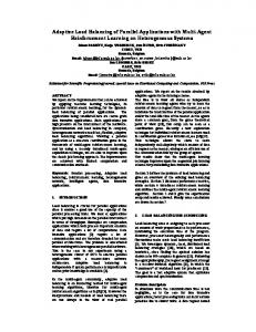
all other cores. Our load balancing scheme ensures that we distribute the overall load as equally as possible taking into consideration the new frequency scaled core speeds. In order to analyze the effectiveness of our scheme, we used Projections [28], a performance analysis tool from the Charm++ infrastructure. Figure 4 demonstrates the timelines and corresponding utilization for all 8 cores throughout the execution. Both the runs in the figure had DVFS enabled. The difference is that the upper run i.e. the top 8 lines, executed Jacobi2D without temperature aware load balancing whereas the lower part i.e. the bottom 8 lines, repeated the same execution with temperature aware load balancing. The

Wave2D w/o TempLB TempLB 1.37 1.26 1.19 1.15

1.22 1.12 1.09 1.05

Mold3D w/o TempLB TempLB 1.39 1.18 1.13 1.05

1.18 1.08 1.06 1.02

maximum temperature threshold for both the runs was 58 ◦ C. Each of the 8 lines for a run represents the timeline for a core and the white patches represent idle time. It can be seen that without temperature aware load balancing (top part of Figure 4), cores 0-3 (lines 0-3) remain idle for a considerable time after some initial iterations. This is due to temperature of the other chip, having cores 4-7 (lines 4-7), exceeding 58 ◦ C resulting in its frequency dropping to 1.6GHz. After the frequency change, both chips work at different speeds but the amount of work assigned to each one of them is the same. Hence cores 0-3 complete the work quickly and spend the rest of the time idle waiting on cores 4-7. After a few more

TABLE IV N ORMAILZED E NERGY FOR DIFFERENT M AXIMUM T EMPERATURE THRESHOLDS Max. Threshold( ◦ C)

Jacobi2D w/o TempLB TempLB

58 62 65 68

CPU Utilization(%) Power(W)

1.04 1.02 1.01 0.99

240

60

180

40

120

20

60

Wave2d

Mol3d

1.20 1.09 1.05 1.02

1.05 1.01 1.01 0.99

Fig. 4. Projections timeline with and without Temperature Aware Load Balancing for Jacobi2D

0

CPU utilization and average power consumption

iterations, the idle times disappear (white patches) because of cores 4-7 getting cooler and restoring the frequency to maximum i.e. 2.53GHz. In the lower part of the figure, notice that our temperature aware load balancing avoids these idle times. As a consequence of this, we end up with a smaller execution time depicted by the smaller timeline for the lower part of Figure 4. In order to get a closer look, we magnified the area enclosed in the rectangle in Figure 4 and present it in Figure 5. Here, we can see the actual difference the frequency change is making. Figure 5 shows 2 iterations with each block representing a task. We highlighted some of the tasks by changing their color so that it is easy to get an idea of the block length i.e. execution time for that task. It can be seen that the blocks on cores 0-3 are smaller than the blocks on cores 4-7 even though they should be equal because the amount of computation in all the tasks is exactly the same. This difference is the result of the different frequencies they are operating at. The average execution time for a task on cores 0-3 is 28.13 ms compared to 35.54 ms on cores 4-7. Hence, this results in cores 0-3 waiting for cores 4-7 shown by the white lines towards the end of each iteration. B. Hot spots Avoidance In order to show the effectiveness of our scheme regarding hot spot avoidance, we ran Jacobi2D for 1000 iterations on 8 cores with temperature aware load balancing invoked after every 10 iterations. All runs conducted for this part took more than 20 minutes. Figure 7 shows a comparison of the average temperatures of all 8 cores for three different runs. Without TempAwareLB represents a run without DVFS implying all

Fig. 5.

Zoomed Projections timeline for 2 iterations

265

Power Comsumption Best Fit

260 Power Consumption (W)

Fig. 3.

Jacobi

1.04 1.00 1.00 0.99

300

80

0

1.12 1.08 1.06 1.04

Mold3D w/o TempLB TempLB

Power (W)

CPU Utilization (%)

100

1.13 1.10 1.06 1.05

Wave2D w/o TempLB TempLB

255 250 245 240 235 230

Fig. 6.

45

50

55 60 65 70 Average Temperature (C)

75

80

Power consumption with varying temperature for Jacobi2D

8 cores running at maximum frequency whereas the other two use our temperature aware load balancing with maximum temperature thresholds of 59 ◦ C and 63 ◦ C. These averages are further averaged over the last 10 iterations. Figure 7 highlights the effectiveness of our scheme in terms of its ability to control the average temperature. This behavior is desirable considering that temperature and power consumption of the machine are directly related. In order to demonstrate the temperaturepower relation, we did a simple experiment in which we executed Jacobi2D at maximum frequency without DVFS for ten minutes and monitored the power consumption of the machine. Since Jacobi2D has a very good load balance, the discrepancy in the power consumption could only be explained in terms of an increase in leakage consumption caused by the

75

Without TempAwareLDB TempAwareLDB Max=63C TempAwareLDB Max=59C

Average Temperature (C)

70

65

60


12 10 8 6 4 2 0

Fig. 8.

0

200

400 600 Iteration Number

800

1000

Standard deviation of core temperatures for Jacobi2D

14

Max Difference in Temperature (C)

where p is the power consumption for all 8 cores and t is the average core temperature. Note that this equation is dependent on CPU utilization of the application and would be different for different applications. The temperature power relation shows us that for every 10 ◦ C increase in the temperature, we should expect a 8.3W increase in power. Another important observation is that the temperature increase can account for up to 9% of extra power consumption by the machine (as evident from maximum and minimum power readings of Figure 6). This can be a very high number considering the overall power consumption of large data centers.

14

Standard Deviation (C)

temperature increase. The results of this experiment in Figure 6 show that there exists a linear relation between temperature and power consumption for Jacobi2D. This relationship can be modeled by: p = 0.83t + 196.5 (4)


12 10 8 6 4 2

55 0 50

45

0

Fig. 7.

200


800

1000

Average core temperature for Jacobi2D

Maintaining the same temperature over the entire machine room is another desirable feature. Our approach ensures that each core obeys the temperature bounds and while doing so, it makes all the cores work in very close temperature range. Not only are we able to keep the average temperature down, we are also able to keep the standard deviation amongst all the cores down to a small number (3 ◦ C). Figure 8 shows the standard deviation of temperature for all 8 cores for the same run as Figure 7. It is evident that the standard deviation increases after 200 iterations in the case where we do not use temperature aware load balancing. This difference keeps on increasing till the 800th iteration. On the other hand, the two runs using our scheme, keep the standard deviation in between 3 − 4 ◦ C, a reduction by a factor of 3. Although the above statistics show that we are able to reduce the deviation in temperatures, it does not guarantee avoidance of hot spots. There might be cases where, out of a 100 racks, only one is working at a very high temperature. In that case, the standard deviation might be low. To deal with this possibility and verify the prevention of hot spots, we also measured the maximum difference in temperature that any core had from the average temperature at each iteration. Figure 9 shows this maximum difference for the same run as

0

200


800

1000

Fig. 9. Maximum difference of core temperatures from average for Jacobi2D

Figure 7. It verifies our claim of hot spot avoidance as the maximum difference using our scheme stays close to 4 ◦ C whereas without our scheme, this difference reaches up to 10 ◦ C. This shows that we were able to bring the maximum temperature difference down by a factor of almost 2.5X. V. C ONCLUSIONS AND F UTURE W ORK We devised a new temperature aware load balancing strategy that uses DVFS to constrain core temperatures. Our results show that it was effective for applications having different power profiles. As far as we know, this is the first work presenting a scheme for temperature aware load balancing in parallel applications whose aim is to reduce cooling costs and the occurrence of hot spots. Another novel feature of our scheme is that it makes run time decisions and does not require any pre runs of the application to gather information a priori. Our future goals include extending this work to more than 8 cores and refining the load balancing such that not all the tasks need to be exchanged across all the cores. We intend to use diffusion load balancing where the hot cores diffuse extra work to their neighbors. In addition, we are planning to work with parallel applications which can be modeled effectively by a Directed Acyclic Graph (DAG) so that we load balance tasks according to their priorities i.e. whether they lie on the critical path or not. Finally, we also plan to exploit the possibility of

making a core sleep if its temperature increases and wake it up at a later time. This could result in a lot of energy savings as we can avoid both the static power as well as the dynamic power. ACKNOWLEDGMENTS We are thankful to Philip Miller for helping us with technical knowledge of Charm++ and sytem administrative work. We also thank Dr. Gengbin Zheng for his valuable input related to Charm++ load balancers. R EFERENCES [1] D. Atwood and J. G. Miner, “Reducing data center cost with an air economizer,” IT at Intel. 2008. [2] R. Mullins, “Hp service helps keep data centers cool,” IDG News Service, Tech. Rep., July 2007. http://www.pcworld.com/article/id,135052/article.html. [3] U. S. Congress, “H.r. 5646 [109th]: To study and promote the use of energy efficient computer servers in the united states,” 2006. [Online]. Available: http://www.govtrack.us/congress/bill.xpd?bill=h109-5646 [4] V. JEDEC Solid State Technology Association, Arlington, “Failure mechanisms and models for semiconductor devices,” in JEDEC publication JEP122C, 2006., 2006. [5] R. Viswanath, V. Wakharkar, A. Watwe, V. Lebonheur, M. Group, and I. Corp, “Thermal performance challenges from silicon to systems,” 2000. [6] C. J. M. Lasance, “Thermally driven reliability issues in microelectronic systems: status-quo and challenges,” Microelectronics Reliability, vol. 43, no. 12, pp. 1969 – 1974, 2003. [7] M. Santarini, “Thermal integrity: A must for low-power ic digital design,” EDN, pages 37-42, Sept. 2005. [8] A. K. Coskun, T. S. Rosing, and K. Whisnant, “Temperature aware task scheduling in mpsocs,” in Proceedings of the conference on Design, automation and test in Europe, ser. DATE ’07. San Jose, CA, USA: EDA Consortium, 2007, pp. 1659–1664. [9] A. Banerjee, T. Mukherjee, G. Varsamopoulos, and S. Gupta, “Coolingaware and thermal-aware workload placement for green hpc data centers,” in Green Computing Conference, 2010 International, 2010, pp. 245 –256. [10] J. Choi, C.-Y. Cher, H. Franke, H. Hamann, A. Weger, and P. Bose, “Thermal-aware task scheduling at the system software level,” in Low Power Electronics and Design (ISLPED), 2007 ACM/IEEE International Symposium on, 2007, pp. 213 –218. [11] “Green hpc - dynamic power management in hpc,” HPC Advisory Council. [Online]. Available: http://www.hpcadvisorycouncil.com/pdf/ vendor content/Platform\%20HPCgreenWP.pdf [12] “Synjet: Low-power green cooling,” http://www.nuventix.com/files/ uploaded files/Low%20Power%20Cooling.pdf. [13] L. Kalé, “The Chare Kernel parallel programming language and system,” in Proceedings of the International Conference on Parallel Processing, vol. II, Aug. 1990, pp. 17–25. [14] C. Bash and G. Forman, “Cool job allocation: measuring the power savings of placing jobs at cooling-efficient locations in the data center,” in 2007 USENIX Annual Technical Conference on Proceedings of the USENIX Annual Technical Conference. Berkeley, CA, USA: USENIX Association, 2007, pp. 29:1–29:6. [15] L. Parolini, B. Sinopoli, and B. H. Krogh, “Reducing data center energy consumption via coordinated cooling and load management,” in Proceedings of the 2008 conference on Power aware computing and systems, ser. HotPower’08. Berkeley, CA, USA: USENIX Association, 2008, pp. 14–14. [Online]. Available: http://portal.acm.org.proxy2. library.uiuc.edu/citation.cfm?id=1855610.1855624 [16] Q. Tang, S. Gupta, and G. Varsamopoulos, “Energy-efficient thermalaware task scheduling for homogeneous high-performance computing data centers: A cyber-physical approach,” Parallel and Distributed Systems, IEEE Transactions on, vol. 19, no. 11, pp. 1458 –1472, 2008. [17] L. Wang, G. von Laszewski, J. Dayal, and T. Furlani, “Thermal aware workload scheduling with backfilling for green data centers,” in Performance Computing and Communications Conference (IPCCC), 2009 IEEE 28th International, 2009, pp. 289 –296.

[18] L. Wang, G. von Laszewski, J. Dayal, X. He, A. Younge, and T. Furlani, “Towards thermal aware workload scheduling in a data center,” in Pervasive Systems, Algorithms, and Networks (ISPAN), 2009 10th International Symposium on, 2009, pp. 116 –122. [19] Q. Tang, S. Gupta, D. Stanzione, and P. Cayton, “Thermal-aware task scheduling to minimize energy usage of blade server based datacenters,” in Dependable, Autonomic and Secure Computing, 2nd IEEE International Symposium on, 2006, pp. 195 –202. [20] D. Rajan and P. Yu, “Temperature-aware scheduling: When is systemthrottling good enough?” in Web-Age Information Management, 2008. WAIM ’08. The Ninth International Conference on, 2008, pp. 397 –404. [21] J. C. Phillips, G. Zheng, S. Kumar, and L. V. Kalé, “NAMD: Biomolecular simulation on thousands of processors,” in Proceedings of the 2002 ACM/IEEE conference on Supercomputing, Baltimore, MD, September 2002, pp. 1–18. [22] A. Merkel and F. Bellosa, “Balancing power consumption in multiprocessor systems,” in Proceedings of the 1st ACM SIGOPS/EuroSys European Conference on Computer Systems 2006, ser. EuroSys ’06. ACM. [23] J. Yang, X. Zhou, M. Chrobak, Y. Zhang, and L. Jin, “Dynamic thermal management through task scheduling,” in Performance Analysis of Systems and software, 2008. ISPASS 2008., 2008. [24] A. Kumar, L. Shang, L.-S. Peh, and N. Jha, “Hybdtm: a coordinated hardware-software approach for dynamic thermal management,” in Design Automation Conference, 2006 43rd ACM/IEEE, 2006, pp. 548 –553. [25] B. Rountree, D. K. Lowenthal, S. Funk, V. W. Freeh, B. R. de Supinski, and M. Schulz, “Bounding energy consumption in large-scale mpi programs,” in Proceedings of the ACM/IEEE conference on Supercomputing, 2007, pp. 49:1–49:9. [26] H. Hanson, S. Keckler, R. K, S. Ghiasi, F. Rawson, and J. Rubio, “Power, performance, and thermal management for high-performance systems,” in IEEE International Parallel and Distributed Processing Symposium (IPDPS), 2007, pp. 1 –8. [27] G. Zheng, “Achieving high performance on extremely large parallel machines: performance prediction and load balancing,” Ph.D. dissertation, Department of Computer Science, University of Illinois at UrbanaChampaign, 2005. [28] L. V. Kalé and A. Sinha, “Projections: A preliminary performance tool for charm,” in Parallel Systems Fair, International Parallel Processing Symposium, Newport Beach, CA, April 1993, pp. 108–114. [29] L. V. Kale and G. Zheng, “Charm++ and AMPI: Adaptive Runtime Strategies via Migratable Objects,” in Advanced Computational Infrastructures for Parallel and Distributed Applications, M. Parashar, Ed. Wiley-Interscience, 2009, pp. 265–282.