Statistical approach utilizing neural networks for CD error prediction Masafumi Asano*, Masaki Satake, Satoshi Tanaka, and Shoji Mimotogi Process & Manufacturing Engineering Center, Semiconductor Company, Toshiba Corporation 8, Shinsugita-cho, Isogo-ku, Yokohama 235-8522, Japan
ABSTRACT We studied a three-layer backpropagation neural network to describe nonlinear relationships between inputs (error sources/control knobs) and output CDs. The application of the neural network to modeling of optical proximity effect for a 65nm node CMOS gate layer was investigated. The prediction accuracy of the neural network was improved with the increase in the training data size, becoming higher than that of a conventional lithography simulation with a lumped parameter model. The result suggests that neural networks trained with a sufficient amount of data can provide the same or higher accuracy for the CD error prediction than physical model-based approaches. The use of information of aerial images as input parameters improved the accuracy. Also, pattern density effects, which are difficult to treat by a conventional lithography simulation, could be successfully reflected in the CD error prediction. Using lot data over a period of time, we trained a neural network in which the exposure parameters and lot mean CDs were inputs and outputs, respectively. From the network, lot mean CDs for successive periods were able to be predicted. From these results, we conclude that the application of neural networks for CD control in advanced lithography is worth developing. Keywords: lithography, critical dimension control, neural networks, optical proximity effect
1. INTRODUCTION To successfully achieve critical dimension (CD) control such as optical proximity correction (OPC) and advanced process control (APC), robust methodologies for CD error prediction are needed. Prior to applying the control, it is necessary to prepare relationships between inputs (i.e., error sources, control knobs) and output CDs represented as mathematical formulas, lookup tables or physics-based simulation models. However, numerous factors influence CD. In particular, in low k1 lithography, even factors that were once considered to have negligible influence on CD because depth of focus (DOF) and exposure latitude (EL) are severely limited. This situation makes it difficult to describe the relationships. For predicting the future, statistical approaches such as multiple regression are widely used in every field of business and industry. The approaches systematically find a rule from past data, and are effective for cases where there is a large number of past data but the physical theory is unknown. Because the relationship from past to future described by the approaches is generally expressed by mathematical formulas, the process of prediction is an easy task. In this work, we treat neural networks as one of the statistical approaches and apply them to predict CD error caused by numerous factors. Neural networks are attractive tools to describe complex relationships between inputs and outputs. In the field of lithography, there have been some reports on the application of neural networks to OPC or process modeling. 1-5 It seems, however, that the number of case studies is small compared with those in fields other than semiconductor manufacturing. We expect neural networks to play important roles in data analysis and CD prediction tools. This paper reports on the applications of neural networks to CD error prediction from two perspectives, namely, modeling of optical proximity effect (OPE) and run-to-run CD variation.
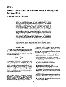
2. NEURAL NETWORK APPROACH We use a three-layer backpropagation neural network to describe nonlinear relationships between inputs (error sources/control knobs) and output CDs. The neural network consists of input, hidden and output layers as shown in Fig. 1. Input signals travel in one direction from the input layer to the output layer via the hidden layer so that the network is *E-mail:
[email protected] Metrology, Inspection, and Process Control for Microlithography XXI, edited by Chas N. Archie Proc. of SPIE Vol. 6518, 651812, (2007) · 0277-786X/07/$18 · doi: 10.1117/12.712115
Proc. of SPIE Vol. 6518 651812-1
called a feed-forward neural network. The input signals are buffered into nodes in the input layer and output responses through the network are delivered from nodes in the output layer. Each node in the hidden layer is connected to every node in the input and output layers. Each connection has its own strength represented by a weight. The mapping from the input layer (node# xi, i=1 to n) to the hidden layer (node# hj, j=1 to h) is achieved with a differentiable nonlinear monotonically increasing function. The following indicates the mapping with a sigmoid function
( H ( X ) = 1 [1 + exp(− X )] ), which is generally used as the transfer function. n ⎛ ⎞ h j = H ⎜ β j + ∑ α ij xi ⎟ , i =1 ⎝ ⎠
(1)
where αij and βj are the coefficients determined in the training. The αij means the weight of the connection, which determines the speed of signal transfer from xi to hj. The βj can be regarded as a weight with respect to the response sensitivity of hj to the transferred signal. On the other hand, the mapping from the hidden layer to output layer (node# yk, k=1 to m) is typically carried out with a linear combination as follows: h
yk = δ k + ∑ γ jk h j ,
(2)
j =1
where γjk and δk are also the weight coefficients. As the weights (αi~δk), random values are initially given so that the network without the training provides unreasonable outputs. By the training, in which the correct answer (input signals and corresponding outputs are known) is given to the network, the weights are adjusted by the backpropagation algorithm so that the difference between the correct outputs and network outputs are minimized. A disadvantage of the algorithm is that the answer is sometimes given to local minima instead of global minima. For the details of the algorithm, refer to the specialized literature.6 The principal reason that we chose the neural network is that it can approximate any continuous nonlinear transformation.7 However, there are several difficulties in the actual use of the neural network. One of the issues is how to decide the number of hidden nodes, which strongly effects on the approximation accuracy. There is no solid rule on the decision. In this work, we decided the number of hidden nodes with trial and error.
Input layer
Hidden layer
h1 x1 x2 xi xn
h2
hj
hh
Output layer
y1 y2 yk ym
Fig. 1. Diagram of a three-layer backpropagation neural network.
Proc. of SPIE Vol. 6518 651812-2
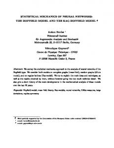
3. MODELING OF OPTICAL PROXIMITY EFFECT The application of neural networks to modeling of OPE for a 65nm node CMOS gate layer was investigated. The experimental exposure was carried out on an ArF scanner with an alternating phase shift mask. The dose and focus were intentionally changed from shot to shot. The printed wafer pattern CDs were measured with a CD-SEM. In our first trial, the input parameters to the neural network are selected from mask design. As shown in Fig. 2, target gate length (L), space to neighboring line (S) and height of phase shifter (H) intentionally varied in the mask were used as the input parameters. The outputs were the gate lengths of the printed wafer resist pattern. The structure of the network is shown in Fig. 3. The training data were randomly sampled from all of the CD measurement data (all: 4200 points) across different mask designs and exposure conditions.
L H
π
0
S Fig. 2. Mask layout of the alternating phase shift mask. The gate length (L), spaces to neighboring line (S), and shifter height (H) are used as input parameters for the neural network.
Input layer
Hidden layer
Output layer
L S
h1
H
h2
E
CD
h3
F Fig. 3. Diagram of the neural network. For comparison, conventional lithography simulations with a lumped parameter model8 were performed in the same way that the lumped parameters were determined with the sampled data. The metric for CD error prediction was root-mean-square (RMS) between the predicted CD and the measured CD
Proc. of SPIE Vol. 6518 651812-3
%RMS of minimum target
including patterns that were not used in the training. Figure 4 shows the sample (training data) size dependence on %RMS, which is normalized by minimum target size, for the neural network and the conventional lithography simulation.
10 7.5 Lithography simulation
5 Neural network
2.5 0 10
100
1000
10000
Training data size Fig. 4. Sample (training data) size dependence on RMS for CD error prediction with the neural network and lithography simulation. The RMS is normalized by minimum target line. The lithography simulation provides higher accuracy at the small sample size, and the accuracy is mostly independent of sample size. On the other hand, the prediction accuracy of the neural network is improved with the increase in the sample size for the training, becoming higher than that of the simulation. Exactly speaking, training data size itself does not necessary make the quality of neural networks higher. The most important factor is whether a selected training data encompasses the parameter space of interest. It is not our intention to conclude that neural networks are better than conventional approaches. The lithography simulator still has room for improvement of prediction accuracy. But the result suggests that with a sufficient amount of training data neural networks can predict OPE with accuracy comparable to that of physical model-based approaches. To further improve CD prediction, input parameters to the neural network were increased. As the new parameters, edge slope and linewidth at a given threshold of aerial images were prepared by an optical simulation. Also, pattern densities (resist open ratios) were calculated based on mask layout. Figure 5 and 6 explain the new parameters. The tested neural network diagrams are shown in Fig. 7. In these tests, CD data at the best dose/focus exposure shot were used. The training was carried out with 100 points randomly sampled and each trained network was evaluated with respect to 300 points, including data that were not used in the training.
Proc. of SPIE Vol. 6518 651812-4
Intensity
Ith Slope
CD
Position
Fig. 5. Aerial image obtained with an optical simulation. Edge slope and linewidth threshold at an intensity Ith are used as input parameters.
4µm x 4µm 2µm x 2µm
Pattern
6µm x 6µm 10µm x 10µm 14µm x 14µm 20µm x 20µm
Fig. 6. Range of pattern density calculation. Resist open ratio for six ranges surrounding pattern of interest is calculated based on mask layout.
Proc. of SPIE Vol. 6518 651812-5
(A) h1
S
h2
S
L
(C)
L CD
H
h3
h1
Slope
H
Optical CD h2
2µm x 2µm
(B)
CD
4µm x 4µm
L S
h1
H
h2
Slope
CD
Pattern density
6µm x 6µm
h3
10µm x 10µm 14µm x 14µm
h3
Optical CD
20µm x 20µm
Fig. 7. Diagrams for tested neural networks: (A) Inputs: Mask design (L, S and H); (B) Inputs: Mask design + aerial image information (edge slope and optical CD); (C) Inputs: Mask design + aerial image information + pattern densities.
%RMS of minimum target
As shown in Fig. 8, the use of information of aerials images as input parameters improves CD error prediction accuracy. This method involves the combined use of physical model and neural network. The pattern density effects, which are difficult to treat by a conventional lithography simulation based on a lumped parameter model, can be reflected successfully in the CD error prediction.
5 4
+ Aerial image information
3
+ Aerial image +Pattern density
2 1 0
(A)
(B)
(C)
Fig. 8. Comparison of %RMS among tested neural networks.
4. LOT CD PREDICTION In state-of-the-art exposure tools, exposure logs can be collected easily via intranet or LAN. From the exposure logs, we chose parameters that are a potential cause of CD errors, such as synchronization error, auto focus control parameter, and some mechanical parameters. Using lot data over a period of time, we trained a neural network in which the exposure parameters and lot mean CDs are inputs and outputs, respectively. Lot mean CDs for successive periods were predicted
Proc. of SPIE Vol. 6518 651812-6
dCD[nm]
by inputting the exposure logs into the trained network. Figure 9 shows lot mean CDs variation. In the last half of the graph, the predicted CDs and actual CDs are compared. The predicted error RMS is 2.0 nm. Some applications of this approach can be expected. One of the applications is to decrease sample size in inline CD metrology. From logs, we may estimate CD distribution in a lot, resulting in high accuracy of APC. In such a case, we need not be bothered by the CD sampling plan.9, 10
8 6 4 2 0 -2 -4 -6 -8
Neural network Actual
RMS ~2nm
training 1
50
100
Lot# Fig. 9. Comparison between the predicted CD error with neural network and actual CD. In the last half, lot CDs are predicted by the neural network trained with the prior 50 lots.
5. CONCLUSION We have demonstrated a method of CD error prediction based on neural networks. A three-layer backpropagation neural network was applied to predict CD error caused by OPE. The prediction accuracy depends on the training data size. With a sufficient amount of training data, the trained neural network can provide the same or higher accuracy for OPE prediction than a conventional lithography simulation. To use information of aerial images and pattern density, which is difficult to treat by a conventional simulation, as input parameters to the neural network is effective for improving CD prediction accuracy. Run-to-run CD variation can also be predicted by neural networks with exposure logs as input parameters. From these results, we conclude that the neural networks for CD control in advanced lithography are worth developing.
ACKNOWLEDGMENTS The authors wish to thank the following people in Toshiba Corporation: Hideki Kanai, Hiroharu Fujise and Hiroshi Matsushita for provision of experimental data; Shizuo Sawada and Soich Inoue for helpful discussion and support for this work.
References 1. P. Jedrasik, “Neural networks application for OPC (Optical Proximity Correction) in mask making,” Microelectron. Eng. 30, 161 – 164 (1996). 2. M. Mahendra, and T. F. Krile, “Applications of neural networks in IC lithography”, Proc. SPIE 2760, 702-712 (1996). 3. V. Mardiris, I. Karafyllidis, D. Soudris, and A. Thanailakis, “Neural networks for the simulation of photoresist exposure process in integrated circuit fabrication”, Modelling Simul. Mater. Sci. Eng. 5, 439-450 (1997). 4. L. Cazzanti, M. Khan, and F. Cerrina, “Parameter extraction with neural networks”, Proc. SPIE 3332, 654-664 (1998).
Proc. of SPIE Vol. 6518 651812-7
5. F. Zach, “Neural network based approach to resist modeling and OPC”, Proc. SPIE 5377, 670-679 (2004). 6. N. Baba, F. Kojima, and S. Ozawa, Neural Networks in Theory and Applications (in Japanese), Chapter 2, Kyoritsu Shuppan, Tokyo, 1994. 7. G. Cybenko, “Approximation by superpositions of a sigmoidal function”, Math. Control Signals Systems, 2, 303-314 (1989). 8. M. Satake, A. Mimotogi, S. Tanaka, S. Mimotogi, K. Hashimoto, and S. Inoue, “Assessment of wafer pattern prediction accuracy by introducing effectively equivalent mask patterns”, Proc. SPIE 6283, 62831B, (2006). 9. M. Asano, and T. Ikeda, “Sampling plan optimization for critical dimension metrology”, J. Microlithogr., Microfabr., Microsyst. 5(3), 033008 (2006). 10. M. Asano, T. Ikeda, T. Koike, and H. Abe, “Evaluation of producer's and consumer's risks in scatterometry and scanning electron microscopy metrology for inline critical dimension metrology”, J. Microlith., Microfab., Microsyst. 5(4), 043006 (2006).
Proc. of SPIE Vol. 6518 651812-8