Statistical-Based Forecasting of Avalanche Prediction

L.

Defence Science Journal, Vol 49, No 5, October 1999, pp. 447-455 O 1999, DESIDOC

Statistical-Based Forecasting of Avalanche Prediction K. Srinivasan Snow & Avalanche Study Establishment, Manali- 175 103.

Girish Semwal GB Pant University, Pantnagar-263 145.

and

T. Sunil Snow & Avalanche Study Establishment, Manali-175 103. ABSTRACT This paper describes the study carried out to predict few meteorological parameters of the next day using the observed parameters of previous day through statistical methods. Multiple linear regression model was formulated for a hill station, Patsio, situated between Manali and Leh, for two winter months (December and January) separately. Twelve meteorological parameters were predicted using 18 predictors observed on the previous day. Ten years data has been used for the computation of regression coefficients. A comparison of the forecasted parameters with the observations was made through the regression model. The prediction of the developed regression model was reasonably close to the observations. The relevant statistical error associated with the linear model (standard error) was also estimated. The output of this regression model will be useful in developing knowledge-based and statistical-based avalanche forecasting model.

1. INTRODUCTION Snow & Avalanche Study Establishment (SASE) is primarily involved in prediction of avalanches in north-west Himalayas and to forewarn the troops and civilian population of the impending avalanche danger. In this, a large area of north-west Himalayas comprising 1 1 major road axes and numerous tracks are covered. In regular avalanche forecasting, the current stability of snow on slopes is analysed and its future stability is assessed after subjecting it to forecasted weather situation to predict the likely release of avalanches in a given time frame. Apart from conventional and process-oriented methods of avalanche predicticn, statistical and knowledgeRevised 01 September 1999

based expert system models are being developed for prediction of avalanches. These models require quantitative forecast of various meteorological parameters at various sites/observatory locations. Hence, an attempt has been made to predict certain meteorological parameters based on 10 years data collected over a station using statistical techniques. Narasimhan and Ramdas' investigated the possibility of predicting minimum temperature by statistical methods. They used maximum temperature and vapour pressure recorded on the previous afternoon as predictors. Raghavan2, Subbaramayya and Surya Rao3 studied in detail the occurrence of heat and cold wave that prevailed over Indian subcontinent.

DEF SCI J , VOL 49, NO 5, OCTOBER 1999

Since India's economy highly depends on monsoon, longrange forecast of monsoon in India has been studied by several researchers4-" using statistical methods. An attempt has been made by Singhio, et al. to issue semi-qualitative precipitation forecasts for a river catchment using synoptic analogue method. They used 12 years data to issue the forecast with confidence. Attrill, et al. conducted a study to assess day-to-day changes, departure and persistence of minimum temperature and the frequency of cold wave and severe cold wave over Gangtok during winter months. They have formulated regression models to forecast minimum temperature with the knowledge of dew point, cloud amount, maximum and minimum temperatures recorded on the previous day. In the present study, a similar technique has been followed to forecast various meteorological parameters for a hill station on Manali-Leh highway based on observed meteorological parameters of the previous day. The hill station, Patsio (77O 27'E; 32" 15'N), situated 160 km from Manali, serves as one of the principal observatories of SASE for predicting avalanches on Manali-Leh axis. The observatory is located at-3800 m above mean sea level. Severe winter in the hilly terrain which is surrounded by high mountains (great Himalayan range), is directly linked with the eastward passage of western disturbances (WDs).The road generally remains closed due to heavy snow precipitation during winter months. This stqion was chosen for the current study due to two reasons, (i) ten years of good quality data was available in SASE's data and (ii) Patsio serves as a primary observatory redicting avalanches over HP sector. From the observations made from various meteorological parametrs at 0300 GMT and 1200 GMT of a day, 18 parameters were chosen as predictors of regression model. The selected predictors and the time period of data used are described in Section 2. A multiple linear regression method was followed to predict certain meteorological parameters of the next day based on the observations of the previous day.

2. REGRESSION MODEL PREDICTORS The collected snow and meteorologicaI data of Patsio was chosen for analysis. The data collected for the period 1983-84 to 1988-89 and 1992-93 to 1995-96 (10 years of winter months) was found suitable for the study. Among the winter months from November to April, only data for December and January were selected for the present study. 0300 GMT (0830 IST) observations are referred as forenoon (FN) and 1200 GMT (1730 IST) observations are referred as afternoon (AN). A total of 18 parameters considered are: (i) minimum temperature, (ii) maximum temperature, (iii) dry bulb temperature (FN), (iv) dry bulb temperature (AN), (v) relative humidity (FN), (vi) relative humidity (AN), (vii) pressure (FN), (viii) pressure (AN), (ix)wind speed (FN), (x) wind speed (AN), (xi) cloud amount (FN), (xii) cloud amount (AN), (xiii) standing snow (FN), (xiv) standing snow (AN), (XV)snow surface temperature (FN), (xvi) snow surface temperature (AN), (xvii) sunshine duration in a day,, and (xviii) fresh snowfall in a day. The analysis was carried out for the months of December and January separately by considering 10 years data together.

3. METHODOLOGY A multiple linear regression of the form

has been applied with December and January data sets separately. Here, Y is the forecast parameter and X,, X,, ......., Xn (here n=18) represent the observed parameters listed above. The a,, a,, a,, ......: .. , a are the regression coefficients, determined by least squares method using 10 years data. This multiple regression was applied to predict the meteorological parameters of the next day (24 hr forecast). In the computation of regression coefficients, deviations from the mean of forecast parameter is considered instead of forecast parameter. It is not always necessary to consider the deviation from the mean of the parameter in a linear regression.

SRINIVASAN, et cil: SHORT RANGE AVALANCHE PREDICTION USING STATISTICAL METHODS

If the different parameters vary in different orders of magnitude, but the deviations from the mean of the parameters are more or less of the same order, it is better to consider deviations from the mean of the parameter. This may minimise the rounding offltruncation error due to limitation of the computer memory (32 bit164 bit word) in the computation of regression coefficients, when the number of parameters considered in the linear regression are more. The multiple linear regression was fitted separately for December and January to get 24 hr forecast of the following 12 parameters: (a) Fresh snowfall in a day (b) Maximum temperature (c) Minimum temperature (d) Average wind speed (FN) (e) Average wind speed (AN) (f) Cloud amount (FN) (g) Cloud amount (AN) (h) Sunshine hours in a day (i) Standing snow height (FN) ( j ) Standing snow height (AN) (k) Snow surface temperature (FN) (1) Snow surface temperature (AN). Though there are many parameters involved in the prediction of avalanches, among the meteorological parameters, the above 12 parameters are considered to be moJe important. The 18 observed meteorological parameters listed in Section 2 are used as input

:It3

0

-

{ -2 -

3 8-

6 .

-4

-10 -8

-6

-6

-2

o

2

4

6

a

OBSERVED TmX("C)

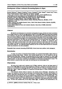
Figure 2. Scatter diagram of observed vs forecasted fresh snowfall in a day in December for maximum temperature.

variables in the multiple linear regression. After computing the regression coefficients, the standard error (SE) is calculated using the following formula:

- 'predicted SE=

i=l

where *obs and 'predicted represent the observed and the predicted parameter, respectively using multiple linear regression and N represents the number of observations considered for the linear regression.

4. RESULTS & DISCUSSION 4.1 Analysis for the Month of December The coefficients of multiple linearkegression for the aforesaid 12 forecast parameters have been estimated based on 10 years data. For December, these are shown in Table 1.

OBSERVED SNOWFALL (cm)

Figure 1. Scatter diagram of observed vs forecasted fresh snowfall in a day in December.

From avalanche forecasting point of view, the quantitative 24 hr forecast of the above 12 parameters is considered to be more important. With the regression coefficients a, (intercept) and a , , a,, ...... a , , (corresponding coefficients of each observed parameter of previous day listed in Section 2), i t is possible to predict quantitatively the above 12 parameters of the next day using the 18 observed -parameters of the previous day. Also, Table 1

Table 1. Computed regression coefficients for the month of December

Sunshine duration (hr)

-3.430 -0.0446 0.0745 0.0120 -0.0331 -0.0343 -0.0105-0.0303 0.6260 -0.1280-0.0004-0.0179 0.1600 -0.0296 -0.0087-0.5470-0.1070 0.1300 1.5100 2.17 'I

Standing snow height

-14.60 -0.0463 -0.0864 0.0368 -0.5450 -0.1530 0.0006 0.23'10 -0.3610 0.0020 -1.718 0.0995 -0.0861 0.0959 1.3500 0.6960 -0.0076 -0.0084 0.4380 3.69

(FN) (cm) Slrading snow height (AN) (cm) %OW

~rfm temperature

-26.00 -0.1080-0.1820 0.0476 -0.7410 -0.0789 -0.0526 -0.0043 1.3800 0.6040 -0.4140 0.1120 @.Oil2 0.190 -0.2550 1.1500 0.3660 0.0183 -1.61004.88 1.940 -0.3220-0.0882-0.0244 0.0401 0.7280 -0.0036 0.0518 0.4430 -0.1540-2.0500 -0.1950 4.372

0.0704 0.1790 3.6600 0.0205 0.0317 0.0802 4.35

(FN) ("C) Snow

1.400 -0.1960-0.0652-0.0454 0.2290 0.0691 0,0093 0.0275 0.4950 -0.0739-0.0649 0.1820 -0.0185-0.0616 0.0322 1.9000 0.1380 -0.0938-1.3600-2.94

SRINIVASAN, el 01: SHORT RANGE AVALANCHE PREDICTION USING STATISTICAL METHODS

0

10

20

30

40

50

OBSERVED SNOWFALL (cm) OBSERVED STANDING SNOW (AN)(cm)

Figure 3. Scatter diagram of observed v s forecasted fresh snowfall in a day in December for standing snow height (AN).

gives SE of each forecast parameter. This SE gives of an average expected error in predicting a parameter using the multiple linear regression method.IFor the month of December, the SE for height of standing snow varies between 3.69-4.88 cm while predicting the standing snow height at FN and AN. The SE of various temperature parameters also varies between 1.57 "C to 2.58 " C . The SE of various other\parameters also seems to be more or less in a reasonable limit. The SE gives the quantitative confidence limits of the forecasted value of various meteorological parameters through this multiple linear regression.

Figure 5. Scatter diagram of observed vs forecasted fresh snowfall in a day in January.

a day and the forecasted value using the above multiple linear regression metho$ are shown as a scatter diagram in Fig.1. In this, the observed values are taken on X-axis and the forecasted values on Y-axis. A line is drawn in diagonal to clearly view the closeness of forecasted and observed values. Mostly the forecasted values are more close to the observed values. The SE for this parameter is 8.83 cm. Similarly, the scatter diagram of observed values against predicted values for maximum temperature, standing snow height (AN), snow surface temperature (AN) are given in Figs 2 and 4,

For December, the observed fresh snowfall in

- 30

A .

-30

-.

--

-25

-20

1

-15

-10

-5

0

5

OBSERVED SNOW SURFACE TEMP (AN) ("C)

Figure 4. Scatter diagram of observed v s forecasted fresh snowfdll in a day in December for snow surface temperature (AN).

-12 -10

-8

-6

-4

-2

0

2

4

OBSERVED Tmx (OC)

Figure 6. Scatter diagram of observed vs forecasted fresh snowfall in a day in January for maximum temperature.

DEF SCI J, VOL 49, NO 5, OCTOBER 1999 \

snow height (FN) and standing snow height (AN) are predicted very close to the observations by the regression model. Since the standing snow height is more linearly dependent on the fresh snowfall amount anh the standing snow height of previous day, both in December and January, this parameter was predicted more close to the observations. Though the figures for other parameters are not given here for brevity, the regression model predicts all the 12 parameters reasonably well. 5. CONCLUSION 0

20

40

60

80

100

120

140

160

OBSERVED STANDING SNOW(AN) (cm)

Figure 7. Scatter diagram of observed vs forecasted fresh snowfallin a day in January for standing snow height (AN).

A multiple linear regression model for individual. months (December and January) has been developed for forecasting certain meteorological parameters with the known values of various meteorological parameters observed on a previous day for a hill station in Himachal Pradesh. The developed

respectively. From Figs 2 and 3, it is evident that the linear regression predicts the standing snow height (AN) and maximum temperature more close to the observed values. From Fig. 4, the forecasted value of snow surface temperature shows a mixed trend of over and less prediction. The SE corresponding to above three parameters are 1.57 "C,4.88 cm and 2.94 "C,'respectively. In general, the linear regression model reasonably well. For brevity, the scatter diagrams of rest of the meteorological parameters are omitted here.

4.2 Analysis for the Month of January Table 2 shows the computed regression coefficients for January for predicting 12 meteorological parameters listed in Section 3. The scatter diagram of the observed and t h e predicted values for fresh snowfall, maximum temperature, standing snow height (AN) and snow surface temperature (AN) are given in Figs 5-8, respectively. From -Fig. 5, the linear model under predicts the snowfall in a day, when observed snowfall is more than 1 0 c m . S E of various parameters for January are almost of t h e same order except few minor changes compared to December. In general, the linear model predicts various meteorological parameters quantitatively close to the observations. Among the 12 selected parameters, the standing

OBSERVED SNOW SURFACE TEMP (AN) (OC)

Figure 8. Scatter diagram of observed vs forecasted fresh snowfall in a day in January for snow surface temperature (AN).

model predicts various snow and meteorological parameters quantitatively and reasonably close to the observations. The predicted meteorological parameters using the above methodology are used as an input to knowledge-based expert system and statistical models to forecast avalanches. Presently, 1 0 years data has been taken into account for computation of regression coefficients. The forecast may further improve if more number of years of such data are considered. However.

SRINIVASAN, et aE:SHORT & A W EAVALANCHE PREDICTION USING STATISTICAL METHODS

DEF SC1 J, VOL 49, NO 5, OCTOBER 1999

the nonlinear variations of observed parameters are not considered. Nevertheless, this simple regression model gives reasonably good qdantitative forecast of certain meteorological parameters.

6. Fleer, H.; Schweitzer, A.B. & Rally, W.Rainfall fluctuations in India and Sri Lanka and largescale rainfall anomalies. Mausam, 1984, 35, 135-44.

REFERENCES

7. Gregory, S(Ed). El Nino years and the spatial pattern of drought over India, 1901-70 in recent climatic change - A regional approach 1988. pp.226-36.

1. Narasimhan, M. & Ramdas, L.A. Indian J. Agric. Sci., 1937, 8(5). 2. Raghavan, K. A climatological study of severe cold waves of India. Indian J. Meteorol. Geophys., 1967, 18 ( I ) , 91-96. 3. Subbaramayya, I. & Surya Rao, D.A. Heat wave and cold wave days in different states of India. Indian J. Meteorol. Hydrol. Geophys., 1976, 27 (4), 436-40. 4. Sikka, D.R. Some aspects of large-scale fluctuations of summer monsoon rainfall over India in relation to fluctuations in the planetary and regional scale circulation parameters. Proc. Ind. Acad. Sci. Earth Planet Science, 1980, 89, 179-95. 5. Mooley, D.A. & Parthasarathy, B.Indian summer monsoon and El Nino. Piire Appl. Geophys., 1983, 121, 339-52.

8. Parthasarathy, B. & Sontakke, N.A. El Ninol SST of Puertochicama and Indian summer monsoon rainfall-statistical relationships. Geo. Int., 1980, 27 (1) 37-58. 9. Mooley, D,A. & Paolino, D.A.(Jr.) The response of the Indian monsoon associated with changes in sea surface temperature over the eastern south equatorial pacific. Mausam, 1989, 40, 369-80. 10. Singh, K. M.; Prasad, M.C. & Prasad, G. Semiquantitative precipitation forecast for river Pun Pun by synoptic anologue method. Mausam, 1995, 46 (2), 149-54. 1 I . Attri, S.D.; Pandya, A.B. & Dubey, D.P.Forecasting of minimum temperarture over Gangtok. Mausam, 1995, 46 (I), 63-68.