1300 Sunnyside Ave., Summerfield Hall, Lawrence, KS 66045-7585, USA. {phgiang ..... called the qualitative expected utility of the lottery in the left-hand side.
Appeared in: A. Darwiche & N. Friedman (eds.), Uncertainty in Artificial Intelligence, 2002, pp. 170-178, Morgan Kaufmann, San Francisco, CA
Statistical Decisions Using Likelihood Information Without Prior Probabilities
Phan H. Giang and Prakash P. Shenoy University of Kansas School of Business 1300 Sunnyside Ave., Summerfield Hall, Lawrence, KS 66045-7585, USA {phgiang,pshenoy}@ku.edu
Abstract This paper presents a decision-theoretic approach to statistical inference that satisfies the Likelihood Principle (LP) without using prior information. Unlike the Bayesian approach, which also satisfies LP, we do not assume knowledge of the prior distribution of the unknown parameter. With respect to information that can be obtained from an experiment, our solution is more efficient than Wald’s minimax solution. However, with respect to information assumed to be known before the experiment, our solution demands less input than the Bayesian solution.
1
Introduction
The Likelihood Principle (LP) is one of the fundamental principles of statistical inference [8, 5, 3, 2]. A statistical inference problem can be formulated as follows. We are given a description of an experiment in the form of a partially specified probability model that consists of a random variable Y which is assumed to follow one of the distributions in the family F = {Pθ |θ ∈ Ω}. The set of distributions is parameterized by θ whose space is Ω. Suppose we observe Y = y, an outcome of the experiment. What can we conclude about the true value of the parameter θ?. Roughly speaking, LP holds that all relevant information from the situation is encoded in the likelihood function on the parameter space. In practice, likelihood information is used according to the maximum likelihood procedure (also refered to as the maximum likelihood principle or method) whereby the likelihood assigned to a set of hypotheses is often taken to be the maximum of the likelihoods of individual hypothesis in the set. The power and importance of this procedure in statistics is testified by the following quote from Lehman [14]:
Although the maximum likelihood principle is not based on any clearly defined optimum consideration, it has been very successful in leading to satisfactory procedures in many specific problems. For wide classes of problem, maximum likelihood procedure have also been shown to possess various asymptotic optimum properties as the sample size tends to infinity. A major approach to statistical inference is the decision-theoretic approach in which the statistical inference problem is viewed as a decision problem under uncertainty. This view implies that every action taken about the unknown parameter has consequences depending on the true value of the parameter. For example, in the context of an estimation problem, an action can be understood as the estimate of the parameter; or in the context of a hypothesis testing problem an action is a decision to accept or reject an hypothesis. The consequences of actions are valued by their utility or loss. A solution to a decision problem is selected according to certain theories. Two widely used decision theories are Wald’s minimax and the expected utility maximization. The latter is appropriate for Bayesian statistical problems in which there is sufficient information to describe the posterior probability distribution on the hypothesis space. Bayesian approach agrees with LP. It holds that the relevant information from the experiment is indeed contained in the likelihood function. However, in addition to the experimental data, Bayesian statistics assumes the existence of a prior probability distribution, which summarizes the information about the unknown parameter before the experiment is conducted. This prior probability assumption is probably the most contentious topic in statistics. In [10, 11], we presented an axiomatic approach to decision making where uncertainty about the true state of nature is expressed by a possibility function. Possibility theory is a relatively recent calculus for describ-
ing uncertainty. Possibility theory has been developed and used mostly within the AI community. It was first proposed in late 1970s by Zadeh [23]. In this paper, we take the position of LP. In particular, we assume that likelihood information, as used in the maximum likelihood procedure, faithfully represents all relevant uncertainty about the unknown parameter. We show that such information is a possibility measure. Thus, our decision theory for possibility calculus is applicable to the problem of statistical inference. We argue that our approach satisfies LP. But, in contrast with the Bayesian approach, we do not assume any knowledge of the prior distribution of the unknown parameter. We claim that our solution is more information efficient than Wald’s minimax solution, but demands less input than the Bayesian solution.
2
Likelihood Information and Possibility Function
Let us recall basic definitions in possibility theory. A possibility function is a mapping from the set of possible worlds S to the unit interval [0, 1] π : S → [0, 1] such that max π(ω) = 1 ω∈S
(1)
Possibility for a subset A ⊆ S is defined as π(A) = max π(ω) ω∈A
(2)
A conditional possibility1 is defined for A, B ⊆ S, π(A) 6= 0 π(A ∩ B) π(B|A) = (3) π(A) Compared to probability functions, the major difference is that the possibility of a set is the maximum of possibilities of elements in the set. Given a probabilistic model F and an observation y, we want to make inference about the unknown parameter θ which is in space Ω. The likelihood concept used in modern statistics was coined by R. A. Fisher who mentioned it as early as 1922 [9]. Fisher used likelihood to measure the “mental confidence” in competing scientific hypotheses as a result of a statistical experiment (see [8] for a detailed account). Likelihood has a puzzling nature. For a single value θ0 , the likelihood is just Pθ0 (y), the probability of observing y if θ0 is in fact the true value of 1
There are two definitions of conditioning in possibility theory. One that is frequently found in possibility literature is called ordinal conditioning. The definition we use here is called numerical conditioning. See [7] for more details.
the parameter. One can write Pθ0 (y) in the form of a conditional probability: P (Y = y|θ = θ0 ). The latter notation implies that there is a probability measure on parameter space Ω. This is the case for the Bayesian approach. In this paper, we do not assume such a probability measure. So we will stick with the former notation. For each value θ ∈ Ω, there is a likelihood quantity. If we view the set of likelihood quantities as a function on the parameter space, we have a likelihood function. To emphasis the fact that a likelihood function is tied to data y and has θ as the variable, the following notation is often used: liky (θ) = Pθ (y)
(4)
Thus, a likelihood function is determined by a partially specified probabilistic model and an observation. It is important to note that the likelihood function can no longer can be interpreted as a probability function. For example, integration (or summation) of the likelihood function over the parameter space, in general, does not sum up to unity. The Likelihood Principle (LP) states that all information about θ that can be obtained from an observation y is contained in the likelihood function for θ given y, up to a proportional constant. LP has two powerful supporting arguments [3]. First, it is well known that likelihood function likY (θ) is a minimal sufficient statistic for θ. Thus, from the classical statistical point of view, the likelihood contains all information about θ. Second, Birnbaum, in a seminal article published in 1962 [4], showed that the Likelihood Principle is logically equivalent to the combination of two fundamental principles in statistics: the principle of conditionality and the principle of sufficiency. The principle of conditionality says that only the actual observation is relevant to the analysis and not those that potentially could be observed. The principle of sufficiency says that in the context of a given probabilistic model, a sufficient statistic contains all relevant information about the parameter that can be obtained from data. Let us define an “extended” likelihood function Liky : 2Ω → [0, 1] as follows: Liky (θ) Liky (A)
def
=
def
=
liky (θ) liky (θ) = ˆ supω∈Ω liky (ω) liky (θ)
(5)
sup Liky (ω) for A ⊆ Ω
(6)
ω∈A
where θˆ is a maximum likelihood estimate of θ. The “extended” likelihood is not new. In fact, it was used by Neyman and Pearson in seminal papers published in 1928 [18] where their famous hypothesis test-
Lik
ing theory was presented. The idea is to use the maximum likelihood estimate as the proxy for a set. Such a procedure is not only intuitively appealing, but it is also backed by various asymptotic optimality properties [13, 15, 19].
0.4
0.3
0.2
If in the process, one decides to focus on a particular subset of the parameter space B ⊆ Ω, the effect of refocusing on the extended likelihood function could be express through what we call conditioning. def
Liky (A|B) =
Liky (A ∩ B) Liky (B)
0.1
y -2
Theorem 1 The extended likelihood function Liky is a possibility function. This technically obvious theorem is important because it establishes a direct link between possibility theory and the central concept in statistics. This relationship has been noticed for quite some time. The fact that the posterior possibility function calculated from a vacuous prior possibility and a random observation behaves as a likelihood function has been pointed out by Smets [21] if the updating process is required to satisfy certain postulates. Dubois et al. [6] show that possibility measures can be viewed as the supremum of a family of likelihood functions. Based on that they justify the min combination rule for possibility functions. We argue further that all relevant information about the unknown parameter that can be obtained from a partially specified probability model and an observation is a possibility measure. This view is essentially Shafer’s idea [20] according to which statistical evidence is coded by belief functions whose focal elements are nested. This kind of belief function (consonant) in its plausibility form is a possibility function. Halpern and Fagin [12] argue for the representation of evidence by a discrete probability function that is obtained by normalizing likelihoods of the singletons so that they sum to unity. However, this probability, Halpern and Fagin concede, should be interpreted in neither frequentist nor subjectivist senses. The identity of likelihood and possibility can be used in two directions. First, for possibility theory and its application in AI, the link with statistics boosts its relevance and validity. We argue that unlike the Bayesian approach, which assumes a completely specified distribution, the possibility function is the result of a partially specified model (true distribution is unknown but assumed to be in a F ) and an observed data. In other words, we have answered the question which is
1
2
3
Figure 1: A Likelihood for Y = 1.4
(7)
We have a theorem whose proof consists of just verifying that the function Liky satisfies the axioms of a possibility measure listed in eqs (1, 2, 3).
-1
often raised in discussions: “Where does possibility information come from?” One answer is it comes from a partially specified probability model of a phenomenon and experimental observations. The derived possibility function encodes all relevant information that can be obtained from the experiment. Second, statistics can also benefit from recently developed techniques in an area that has a different motivation. Traditional problems in statistics may be re-examined in the light of new insights. In the rest of this paper, we study the statistical decision problem from the point of view of qualitative decision theory as described in [10, 11]. Example: A random variable Y is known to have a normal distribution. It is also known that mean µ ∈ {0, 1} and standard deviation σ ∈ {1, 1.5}. Suppose that value y = 1.4 is observed. Construct an extended likelihood function representing information about unknown parameters of distribution of Y . Parameter θ = (µ, σ). Ω = {ω1 , ω2 , ω3 , ω4 } with ω1 = (0, 1), ω2 = (0, 1.5), ω3 = (1, 1), ω4 = (1, 1.5).
lik1.4 (.) Lik1.4 (.)
ω1 0.1497 0.4066
ω2 0.1720 0.4672
Events µ = 0 or {ω1 , ω2 } µ = 1 or {ω3 , ω4 } σ = 1 or {ω1 , ω3 } σ = 1.5 or {ω2 , ω4 } µ = 0|σ = 1 µ = 1|σ = 1 µ = 0|σ = 1.5 µ = 1|σ = 1.5
3
ω3 0.3683 1.0
ω4 0.2567 0.6970
Lik1.4 (.) 0.4672 1. 1. 0.6970 0.4066 1.0 0.6703 1.0
A Decision Theory with Likelihood Information Only
Let us review, in terms of likelihood semantics, our proposal for qualitative decision making with possibility theory [10, 11]. We assume a situation that includes
a set Ω which can be interpreted as the set of hypotheses or the parameter space. Also assumed is a set of consequences or prizes X that includes one best prize (x) and one worst prize (x). An action d is a mapping Ω → X. In other words, the consequence of an action is determined by which hypothesis is true. The set of actions is denoted by A. The uncertainty about hypotheses obtained from the observation is expressed by an extended likelihood function π. An action coupled with a uncertainty measure determines a simple lottery. Each lottery is a mechanism that delivers prizes with associated likelihoods. Formally, a lottery L induced by π and d is a mapping from X → [0, 1] such that L(x) = π(d−1 (x)) for x ∈ X where d−1 is a set-valued inverse mapping of action d. For the remainder of this paper, we will denote a simple lottery by [L(x1 )/x1 , L(x2 )/x2 , . . .] with the convention that those xj for which L(xj ) = 0 are omitted. If we let prizes to be lotteries then we have compound lotteries. If a lottery involves only two prizes x and x (the best and the worst) as potential outcomes then it is called a canonical lottery. The set of canonical lotteries is denoted by Lc . We study a preference relation º on the set of lotteries L. We postulate that º satisfies five axioms similar to those proposed by von Neumann and Morgenstern for the classical linear utility theory (in the form presented in [17]). They are as follows. (A1) Order. º is reflexive, transitive, complete. (A2) Reduction of compound lotteries. Let L = [δ1 /L1 , δ2 /L2 . . . δk /Lk ] and Li = [κi1 /x1 , κi2 /x2 , . . . κir /xr ] then L ∼ Ls where Ls = [κ1 /x1 , κ2 /x2 , . . . κr /xr ] with κj = max {δi .κij } 1≤i≤k
(8)
(A3) Substitutability. If Li ∼ L0i then [δ1 /L1 , . . . δi /Li . . . δk /Lk ] ∼ [δ1 /L1 , . . . δi /L0i . . . δk /Lk ] (A4) Continuity. For each xi ∈ X there is a s ∈ Lc such that xi ∼ s. (A5) Qualitative monotonicity. [λ/x, µ/x] º [λ0 /x, µ0 /x] iff (λ ≥ λ0 )&(µ ≤ µ0 ) (9) In [10, 11] we prove a representation theorem for the preference relation. Theorem 2 º on L satisfies axioms A1 to A5 if and only if it is represented by a unique utility function QU
such that QU([δ1 /L1 , . . . , δk /Lk ]) = max {δi .QU(Li )} 1≤i≤k
(10)
where function QU is a mapping L → U where U = {h u, v i|u, v ∈ [0, 1] and max(u, v) = 1}. The binary utility scale is formed by defining an order ≥ on U as follows (1 ≥ λ ≥ λ0 & µ = µ0 = 1) ∨ 0 0 (λ = 1 & λ0 < 1) ∨ hλ, µi ≥ hλ , µ i iff (λ = λ0 = 1 & µ ≤ µ0 ) Multiplication and maximization are extended to pairs as follows (α, β, γ, ξ are scalar). α.hβ, γi max{hα, βi, hγ, ξi}
def
=
def
=
hα.β, α.γi
(11)
hζ, ηi
(12)
where ζ = max{α, γ} and η = max{β, ξ} The expression in the right-hand side of eq.(10) is called the qualitative expected utility of the lottery in the left-hand side. As a result of theorem 2, we can compare the preference of lotteries by looking at their expected utility. These five axioms were justified on intuitive grounds in [10, 11]. As we argued, the uncertainty information about the unknown parameter resulting from an experiment is captured by a possibility measure. Thus, the axioms can be justified indirectly in the context of statistical inference problem. However, we think it would be useful to reexamine them directly in terms of likelihood here. Among the axioms, A1 and A3 are standard assumptions about a preference relation. A2 is an implication of the conditioning operation. Suppose that the unknown parameter θ is a vector. We can think, for example, θ = (γ, σ). Let us consider a compound lottery L = [π1 /L1 , π2 /L2 , . . . , πk /Lk ] where Li = [κi1 /x1 , . . . , κir /xr ] for 1 ≤ i ≤ k. Underlying L, in fact, is a two-stage lottery. The first stage is associated with a scalar parameter γ. It accepts values γ1 , γ2 , . . . γk with likelihoods π1 , π2 , . . . πk respectively. If γi is the true value, the holder of L is rewarded with simple lottery Li that, in turn, is associated with scalar parameter σ that accepts σoi (1) , σoi (2) , . . . σoi (r) with likelihoods κi1 , κi2 , . . . κir where oi is a permutation of (1, 2, 3, . . . r). When σoi (j) obtains, the holder is rewarded with prize xj . We can view this lottery from a different angle. That is L is a lottery that delivers xj in case tuple < γi σoi (j) > is the true value of θ. Thus, the extended likelihood < γi σoi (j) > is πi .κij since κij is the conditional likelihood on γi . The set of tuples for which xj is delivered is {< γi σoi (j) > |1 ≤ i ≤ k}.
Utility
We just showed that binary utility elicitation is done by betting on a likelihood gamble. We assume that the betting behavior of the decision maker is consistent and rational in some way. For example, paying $0.20 for the gamble if Y = −3 and paying $0.70 if Y = 1 is considered irrational. The constraint we impose is formulated as axiom A5, qualitative monotonicity (x = 1 and x = 0). In other words, we require that the price for the lottery [λ/1, µ/0] is no less than the price for [λ0 /1, µ0 /0] if the condition on the right hand of eq.(9) is satisfied.
1 0.8 0.6 0.4 0.2
-3
-2
-1
1
2
3
Y
Figure 2: Binary utility from observation Thus, the extended likelihood associated with prize xj in lottery L is max{πi .κij |1 ≤ i ≤ k}. The continuity axiom (A4) requires that for any consequence x ∈ X there is a canonical lottery c = (λ1 /x, λ2 /x) such that x ∼ c. For clarity, let us assume that x = 1, x = 0. For any x ∈ [0, 1], we need to find a canonical lottery c equivalent to x. We propose a likelihood gamble for that purpose. By doing so, we provide an operational semantic for the concept of binary utility. Suppose that random variable Y is generated from one of two normal distributions2 that have the same standard deviation σ = 1 but with two different means, either −1 or 1, i.e., Y ∼ N (−1, 1) or Y ∼ N (1, 1). Next you are informed that a randomly observed value of Y is y. What is the most you would be willing to pay for a gamble that pays $1 if the true mean µ is −1 and nothing if the true mean is 1? If the answer is x, then it can be shown that for you x ∼ [Liky (−1)/1, Liky (1)/0]
(13)
Figure 2 plots functions λ1 (y) = Liky (−1) (the dashed line) and λ2 (y) = Liky (1). This betting procedure is quite similar to the test used in practice to identify the unary utility of a monetary value. But there are important differences. First, instead of using a random variable with a known distribution (e.g., tossing a fair coin or rolling a dice), we use for our test a partially specified model together with a randomly generated observation. We let the decision maker bet on a gamble tied to a situation that by nature, is a hypothesis testing problem. The rewards in this gamble are tied not to an observed realization of the random variable as in an ordinary gamble, but instead, the rewards are conditioned on the true value of the parameter underlying the random variable. 2 The use of normal distributions is for illustration purpose only. Any other distribution will do.
Since the likelihood gamble, as noted, is a hypothesis testing problem. We show that axiom A5 is supported by the traditional statistical inference methods namely classical, Bayesian and likelihood. Let us denote by y and y 0 the values of Y that associate with gambles [λ/1, µ/0] and [λ0 /1, µ0 /0] respectively. Referring to the graphs in figure 2, it is easy to check the fact that the condition on the right hand of eq.(9) is equivalent to y ≤ y 0 . We want to show that the confidence in favor of µ = −1 is higher for y than for y0 no matter which methods are used. For the significance test method applied for testing µ = 1 against µ = −1, the p-value for rejecting µ = 1 in favor of µ = −1 provided by data y is Pµ=1 (Y ≤ y) that is smaller than the p-value corresponding to data y 0 which is Pµ=1 (Y ≤ y 0 ). The likelihood reasoning [8] compares the hypotheses by looking at their likelihood ratios. It is obvious that liky (−1) liky 0 (−1) ≥ liky (1) liky 0 (1)
(14)
If the decision maker is Bayesian and assumes the prior probability P (µ = −1) = p, then (s)he will calculate posterior probabilities P (µ = −1|y) =
p.Liky (−1) p.Liky (−1) + (1 − p).Liky (1)
(15)
From Liky (−1) ≥ Liky 0 (−1) and Liky (1) ≤ Liky 0 (1), we have P (µ = −1|y) ≥ P (µ = −1|y 0 ). Let us denote the expected payoffs of the likelihood gambles in two cases Y = y and Y = y0 by Vy and Vy 0 . Vy = P (µ = −1|y).1 + P (µ = 1|y).0 = P (µ = −1|y) ≥ P (µ = −1|y 0 ) = Vy0 . We want to invoke one more, in our opinion the most important, justification for A5. This justification is based on the concept of the first order stochastic dominance (FSD). Without being a strict Bayesian, we do not assume to know the prior probability of P (µ = −1). We can model this situation by viewing the prior probability of µ = −1 as a random variable ρ taking value in the
inequality means Vy (ρ) D1 Vy 0 (ρ). Thus, we have the following theorem
Exp. payoff 1 0.8
Theorem 3 The order on binary utility is the order of first degree stochastic dominance.
0.6 0.4
In summary, we show that there are compelling arguments justifying the five proposed axioms.
0.2 Prior 0.2
0.4
0.6
0.8
1
4 Figure 3: Expected payoffs for two observations unit interval. However, we do not assume to know the distribution of ρ. We will write the expected payoff of the likelihood gamble by Vy (ρ). Since it is a function of ρ, Vy (ρ) is a random variable. We want to compare two r.v. Vy (ρ) and Vy0 (ρ). One of the methods used for comparing random variables is based on the concept of stochastic dominance (SD). We are interested in the first degree stochastic dominance (FSD). This concept has been used extensively in economics, finance, statistics and other areas [16]. Suppose X and Y are two distinct random variables with the cumulative distributions F and G respectively. We say that X stochastically dominates (first degree) Y (write XD1 Y ) iff F (x) ≤ G(x) ∀x. Since X and Y are distinct, strict inequality must hold for at least one value x. FSD is important because of the following equivalence XD1 Y iff E(u(X)) ≥ E(u(Y )) ∀u ∈ U where U the class of non-decreasing utility functions. E(u(X)) is the expected utility of X under utility function u. Let us consider the relation between Vy (ρ) and Vy 0 (ρ). We have the following lemma that relates the expected payoffs and the likelihood pairs. The proof is omitted. Lemma 1 For a given value ρ 6∈ {0, 1}, Vy (ρ) > Vy 0 (ρ) iff hLiky (−1), Liky (1)i > hLiky 0 (−1), Liky 0 (1)i
(16)
In figure 3, the lower curve is the graph for V0.60 (ρ) (at Y = .6 the extended likelihood pair is h.3011, 1.i) and the upper curve is the graph for V0.26 (ρ) (h.5945, 1.i). Now, for any v ∈ (0, 1), let us denote the roots of equations Vy (ρ) = v and Vy0 (ρ) = v by ρv and ρ0v respectively i.e., Vy (ρv ) = v and Vy0 (ρ0v ) = v. If hλ, µi > hλ0 , µ0 i then by lemma 1 Vy (ρv ) > Vy 0 (ρv ). Therefore, Vy 0 (ρ0v ) > Vy0 (ρv ). Because Vy 0 (ρ) is strictly increasing, we infer ρv < ρ0v . Since Vy (ρ) and Vy 0 (ρ) are increasing, P (Vy (ρ) ≤ v) = P (ρ ≤ ρv ) and P (Vy 0 (ρ) ≤ v) = P (ρ ≤ ρ0v ). Because ρv < ρ0v , P (Vy (ρ) ≤ v) ≤ P (Vy 0 (ρ) ≤ v). This last
A Decision-Theoretic Approach to Statistical Inference with Likelihood
We will review the decision theoretic approach to statistical inference. We assume given the set of alternative actions denoted by A, the sample space of Y by Y. A loss L(a, θ) measures the loss that arises if we take action a and the true value of the parameter is θ. A decision rule is a mapping δ : Y → A, that is for an observation y the rule recommends an action δ(y). The risk function of a decision rule δ at parameter value θ is defined as Z def R(δ(Y ), θ) = Eθ L(δ(Y ), θ) = L(δ(y), θ)pθ (y) Y
(17) The risk function measures the average loss by adopting the rule δ in case θ is the true value. The further use of risk functions depends on how much information we assume is available. For each point in the parameter space, there is a value of risk function. In case no a priori information about parameter exists, Wald [22] advocated the use of minimax rule which minimizes the worst risk that could be attained by a rule. (18) δ ∗ = arg min max R(δ, θ) δ∈∆ θ∈Ω
where ∆ is the set of decision rules. δ ∗ is called the minimax solution. If we assume, as the Bayesian school does, the existence of a prior distribution of the parameter then the risk could be averaged out to one number called Bayes risk r(δ) = Eρ R(δ, θ) (19) where ρ is prior distribution of θ. Then the optimal rule is one that minimizes the Bayes risk which is called the Bayes solution. Wald [22] pointed out the relationship between the two rules. There exists a prior distribution ρ called “the least favorable” for which Bayes solution is the minimax solution. In our view, both solution concepts are not entirely satisfactory. Bayes solution is made possible by assuming the existence of prior distribution, which is often a leap of faith. Although in highly idealized situation,
u(a, θ) a1 a2
prior probability may be extracted from preference or betting behavior, in practice, there are many factors that violate conditions necessary for such deduction. We have two problems with Wald’s proposal. First, the risk function has no special role for the actually observed data. Thus, Wald’s proposal does not respect the principle of conditionality. That violation leads to the second problem of minimax rule. The rule ignores information about the parameter that is obtained from the data. One can argue that the minimax rule is being cautious. But it is, in our opinion, too cautious. There is information about the parameter θ provided by the observed data, namely, likelihood information, that must be utilized in making a decision. We propose the following solution. For a given y ∈ Y, an extended likelihood function Liky is calculated. That allows comparison of actions on the basis of their qualitative expected utilities, or more exactly, utilities of lotteries induced by the actions and the likelihood function. For an action d and an observation y, denote Ld (y) the lottery generated. The selected action given observation y is d∗ (y) = arg sup QU(Ld (y))
5
Liky (θ) θ1 θ2
3 In contrast to max defined in eq. 12 that operates on scalars.
θ1 .2 .5
θ2 .7 .5
y1 .1 .7
y2 .4 .2
y3 .5 .1
For each point in the sample space, you can either choose a1 or a2 , so there are 8 possible decision rules in total. Each decision rule specifies an action given an observation. y1 y2 y3
An Illustrative Example
Let us assume that there are only two possible faults i.e., Ω = {θ1 , θ2 } where θ1 means there is the need for cleaning and θ2 means the clock has been physically damaged and the works need replacement. Utility and loss functions are given in the following table. The relationship between utility and loss is through equation Loss = 1 − Utility.
L(a, θ) a1 a2
The manufacturer can ask the customer to provide a symptom of malfunction when a clock is sent to the service center. The symptom can be viewed as observation. Assume the sample space Y = {y1 , y2 , y3 } where y1 means “the clock has stopped operating”, y2 “the clock is erratic in timekeeping and y3 - “clock can only run for a limited period”. Such information gives some indication about θ that is expressed in terms of likelihood
(20)
The following example is adapted from [1]. The manufacturer of small travel clocks which are sold through a chain of department stores agrees to service any clock once only if it fails to operate satisfactorily in the first year of purchase. For any clock, a decision must be made on whether to merely clean it or replace the works, i.e., the set of actions A = {a1 , a2 } where a1 denotes cleaning the clock, and a2 denotes immediately replacing the works.
θ2 .3 .5
The loss table is roughly estimated from the fact that cleaning a clock costs $0.20 and replacing the works costs $0.50. If the policy is to replace the works for every clock needing service then the cost is $0.50 no matter which problem is present. If the policy is to clean a clock first, if the state is θ1 then the service costs $0.20, however in the case of physical damage then cleaning alone obviously does not fix the problem and the manufacturer ends up replacing the works also. Thus the total cost is $0.70.
d∈A
where sup3 is the operation taking maximum element according to the binary order. Equation (20) also defines a decision rule in the sense that for each point in the sample space, it gives an action. We call such a decision rule the likelihood solution for obvious reasons.
θ1 .8 .5
δ1 a1 a1 a1
δ2 a1 a1 a2
δ3 a1 a2 a1
δ4 a1 a2 a2
δ5 a2 a1 a1
δ6 a2 a1 a2
δ7 a2 a2 a1
δ8 a2 a2 a2
We calculate the risk function values for each rule and parameter value in the following table Rij θ1 θ2
δ1 .2 .7
δ2 .35 .68
δ3 .32 .66
δ4 .47 .64
δ5 .23 .56
δ6 .38 .54
δ7 .35 .52
δ8 .50 .50
Notice that there is no rule which is superior to all other for both values of θ. Wald’s minimax solution is δ8 . If we assume prior distribution of θ then we can calculate the Bayes risks for the rules. For example if prior probability p(θ1 ) = .7, then Bayes risks r.7 (δi ) are δ1 .35
δ2 .449
δ3 .442
δ4 .541
δ5 .329
δ6 .428
δ7 .401
δ8 .50
In this case, the Bayes solution is δ5 . It is easy to understand why the Bayes solution will be different if
the prior p(θ1 ) changes. Indeed, a sensitivity analysis shows that Bayes solution is Bayes solution δ1 δ5 δ7 δ8
When p(θ1 ) ≥ .824 .250 ≤ p(θ1 ) ≤ .824 .118 ≤ p(θ1 ) ≤ .250 p(θ1 ) ≤ .118
In our approach, suppose the betting procedure produces the following preference equivalence between monetary values and binary utility. Unary utility .8 .5 .3
Binary utility h1, .25i h1, 1i h.43, 1i
Given observation y1 , the extended likelihood function is Liky1 (θ1 ) = .14 and Liky1 (θ2 ) = 1. Action a1 is associated with lottery La1 (y1 ) = [.14/h1, .25i, 1/h.43, 1i] whose qualitative expected utility is calculated as QU(La1 (y1 )) = = =
max{.14h1, .25i, 1h.43, 1i} max{h.14, .035i, h.43, 1i} h.43, 1i
Action a2 is associated with lottery La2 (y1 ) = [.14/h 1, 1 i, 1/h 1, 1 i] whose qualitative expected utility QU(La2 (y1 )) = h 1, 1 i. Thus, given y1 , we have a2 Ây1 a1 i.e., a2 is strictly prefered to a1 . Given observation y2 , the extended likelihood function is Liky2 (θ1 ) = 1 and Liky2 (θ2 ) = .5. We calculate the qualitative expected utility for a1 is QU(La1 (y2 )) = h1, .5i and for a2 QU(La2 (y2 )) = h1, 1i. Thus, a1 Ây2 a2 . Given observation y3 , the extended likelihood function is Liky2 (θ1 ) = 1 and Liky2 (θ2 ) = .2. The qualitatively expected utility for a1 is QU(La1 (y3 )) = h1, .25i and for a2 remains QU(La2 (y3 )) = h1, 1i. Thus, a1 Ây3 a2 . In summary, our approach suggests δ5 as the likelihood solution. Let us make an informal comparison of likelihood solution with minimax and Bayes solutions. In this example, likelihood solution δ5 is different from the minimax solution δ8 . It is because, as we noted, minimax solution ignores the uncertainty generated by an observation while likelihood solution does not. In that sense, likelihood solution is more information efficient. If the prior probability p(θ1 ) = .7, then the Bayes solution is δ5 the same as the likelihood solution. If prior probability is available, one can argue that Bayes solution is the optimal one. However, the “optimality” of Bayes solution comes at a cost. The decision maker
must possess the prior probability. This condition can be satisfied either at some monetary cost (doing research, or buying from those who know) or the decision maker can just assume some prior distribution. In the latter case, the cost is a compromise of solution optimality. One can extend the concept of Bayes solution to include the sensitivity analysis. This certainly helps decision maker by providing a frame of reference. But sensitivity analysis itself does not constitute any basis for knowing the prior probability. The fact that likelihood solution δ5 coincides with Bayes solution that corresponds to a largest interval of prior should not be exaggerated. Different unarybinary utility conversions may lead to different likelihood solution. However, it is important to note that there is a fundamental reason for the agreement. As we have pointed out, the axioms A1 to A5 on which likelihood solution is based, are structurally similar to those in [17]. In that work, Luce and Raiffa used those axioms to justify linear utility concept which ultimately is a basis for Bayes solution. Thus, at a foundational level, optimality of likelihood solution could be justified in the same way as the optimality for Bayes solution although the two optimality concepts are obviously different. We argue that the question of which optimality has precedence over the other depends on how much information is available.
6
Summary and Conclusion
In this paper, we take the fundamental position that all relevant information about the unknown parameter is captured by the likelihood function. This position is justified on the basis of the Likelihood Principle and various asymptotic optimality properties of the maximum likelihood procedure. We show that such a likelihood function is basically a possibility measure. We re-examine the axioms of our decision theory with possibility calculus in terms of the likelihood semantics. We provide a betting procedure that determines, for a decision maker, the binary utility of a monetary value. This test justifies the continuity axiom. We also justify the monotonicity axiom A5 in terms of first order stochastic dominance. We propose a new likelihood solution to a statistical decision problem. The solution is based on maximizing the qualitative expected utility of an action given the likelihood function associated with a point in the sample space. The likelihood solution is sandwiched by Wald’s minimax solution on one side and the Bayes solution on the other side. Compared to the minimax solution, the likelihood solution is more information efficient. Compared to the Bayesian solution, the likelihood solution does not require a prior probability dis-
tribution of the unknown parameter.
Acknowledgment We thank anonymous referees for comments, reference and suggestions to improve this paper.
References [1] Barnett, V. Comparative Statistical Inference, 3 ed. John Wiley and Sons, New York, Chichester, Brisbane, 1999. [2] Basu, D., and Ghosh, I. Statistical Information and Likelihood: A Collection of Critical Essays by Dr. Basu. Lecture notes in Statistics. Springer-Verlag, New York, Berlin, Heidelberg, 1988. [3] Berger, J. O., and Wolpert, R. L. The Likelihood Principle, 2 ed. Lecture notes-Monograph series. Institute of Mathematical Statistics, Hayward, California, 1988. [4] Birnbaum, A. On the foundation of statistical inference. Journal of the American Statistical Association 57, 298 (1962), 269—306. [5] Cox, D. R., and Hinkley, D. V. Theoretical Statistics. Chapman and Hall, London, 1974. [6] Dubois, D., Moral, S., and Prade, H. A semantics for possibility theory based on likelihoods. Journal of Mathematical analysis and applications 205 (1997), 359—380. [7] Dubois, D., Nguyen, T. H., and Prade, H. Possibility theory, probability and fuzzy sets. In Handbook of Fuzzy Sets Series, D. Dubois and H. Prade, Eds. Kluwer Academic, Boston, 2000, pp. 344—438. [8] Edwards, A. W. F. Likelihood. Cambridge Univesity Press, Cambridge, 1972. [9] Fisher, R. A. On the mathematical foundation of theoretical statistics. Philosophical transactions of the Royal society of London, A 222 (1922), 309—368. Reprinted: Collected Papers of R. A. Fisher vol. 1, ed. J. H. Bennett, University of Adelaide 1971. [10] Giang, P. H., and Shenoy, P. P. A qualitative linear utility theory for Spohn’s theory of epistemic beliefs. In Uncertainty in Artificial Intelligence: Proceedings of the Sixteenth Conference (UAI-2000) (San Francisco, CA, 2000), C. Boutilier and M. Goldszmidt, Eds., Morgan Kaufmann, pp. 220—229.
[11] Giang, P. H., and Shenoy, P. P. A comparison of axiomatic approaches to qualitative decision making using possibility theory. In Uncertainty in Artificial Intelligence: Proceedings of the Seventeenth Conference (UAI-2001) (San Francisco, CA, 2001), J. Breese and D. Koller, Eds., Morgan Kaufmann. [12] Halpern, J. Y., and Fagin, R. Two views of belief: belief as generalized probability and belief as evidence. Artificial Intelligence 54, 3 (1992), 275—318. [13] Kallenberg, W. C. M. Asymtotic Optimality of Likelihood Ratio Tests in Exponential Families, vol. 77 of Mathematical Centre Tracts. Mathematisch Centrum, Amsterdam, 1978. [14] Lehmann, E. L. Testing Statistical Hypotheses, 2 ed. John Wiley and Sons, New York, Chichester, Brisbane, 1986. [15] Lehmann, E. L., and Casella, G. Theory of Point Estimation, 2 ed. Springer Texts in Statistics. Springer, New York, Berlin, Heidelberg, 1998. [16] Levy, H. Stochastic dominance and expected utility: survey and analysis. Management Science 38, 4 (1992), 555—593. [17] Luce, R. D., and Raiffa, H. Games and Decision. John Wiley & Sons, 1957. [18] Neyman, J., and Pearson, E. S. On the use and interpretation of certain test criteria for purposes of statistical inference. part 1. Biometrica 20A (1928), 175—240. In J. Neyman and E.S.Pearson Joint Statistical Papers. University of California Press. 1967. [19] Severini, T. A. Likelihood Methods in Statistics. Oxford Univesity Press, Oxford, 2000. [20] Shafer, G. A Mathematical Theory of Evidence. Priceton University Press, Princeton, NJ, 1976. [21] Smets, P. Possibilistic inference from statistical data. In Proceedings of 2nd World Conference on Mathematics at the service of Man (La Pamas (Canary Island) Spain, 1982), pp. 611—613. [22] Wald, A. Statistical Decision Function. John Wiley and Sons, New York, 1950. [23] Zadeh, L. Fuzzy set as a basis for a theory of possibility. Fuzzy Sets and Systems 1 (1978), 3— 28.