Dec 16, 2010 - Statistical graphics play a crucial role in exploratory data analysis, model checking and diagnosis. Until recently there were no formal visual ...
Visual Statistical Inference for Regression Parameters Mahbubul Majumder, Heike Hofmann, Dianne Cook Department of Statistics, Iowa State University December 16, 2010
Abstract
assessing the performance of individuals on lineup plots [Buja et al., 2009] for testing significance of regression parameters. Section 2 describes the basic ideas of visual inference, Section 3 applies these ideas to the case of inference for regression analysis. In Section 4 we outline the setup for the human-subject study and and present results.
Statistical graphics play a crucial role in exploratory data analysis, model checking and diagnosis. Until recently there were no formal visual methods in place for determining statistical significance of findings. This changed, when Buja et al. [2009] conceptually introduced two protocols for formal tests of visual findings. In this paper we take this a step further by comparing the lineup protocol [Buja et al., 2009] against classical statistical testing of the significance of regression model parameters. A human subjects experiment is conducted using simulated data to provide controlled conditions. Results suggest that the lineup protocol provides results equivalent to the uniformly most powerful (UMP) test and for some scenarios yields better power than the UMP test.
1
2
Visual Statistical Inference
This section outlines the concepts of visual inference in comparison to the procedures of classical statistical inference. Table 1 (derived from Buja et al. [2009]) gives a summarized overview of this comparison. Let θ be a population parameter of interest, with θ ∈ Θ, the parameter space. Any null hypothesis H0 then partitions the parameter space into Θ0 and Θc0 , with H0 : θ ∈ Θ0 versus H1 : θ ∈ Θc0 . Unlike classical hypothesis testing the statistic in visual inference is not a single value, but a plot that is appropriately chosen to describe the parameter of interest, θ. When the alternative hypothesis is true, it is expected that the plot of the observed data, the test statistic, will have visible feature(s) consistent with θ ∈ Θc0 , and that visual artifacts will not distinguish the test statistic as different when H1 is not true.
Introduction
Any statistical analysis must include some statistical graphics. For exploratory data analysis, statistical graphics play an invaluable role in model checking and diagnostics. Even though we have established mathematical procedures to obtain various statistics, we need to support the results by also producing the relevant plots. In recent years we have seen several major advances in statistical graphics. A grammar of graphics introduced by Wilkinson [1999] presents a structured way to generate specific graphics from data and define connections between disparate types of plots. We have modern computing systems like R and SAS that facilitate easy production of high quality statistical plots. Wickham [2009] has implemented a revised version of the grammar of graphics in R, in the package ggplot2. Buja et al. [2009], following from Gelman [2004], proposed two protocols that allow the testing of discoveries made from statistical graphics. This work represents a major advance for graphics, because it bridges the gulf between classical statistical inference procedures and exploratory data analysis. In this paper we present results of a human-subject study
Definition 2.1. A lineup plot is a layout of m visual statistics, consisting of • m − 1 plots simulated from the model specified by H0 (null plots) and • the test statistic produced by plotting the observed data, possibly arising from H1 . If H1 is true, the test statistic is expected to be the plot that is most different from the other plots in the lineup plot. A careful visual inspection should reveal the differences in the feature shown by the test statistic under null and alternative hypothesis. If the test statistic cannot be identified 1
Table 1: Comparison of visual inference with existing inference technique Mathematical Inference Visual Inference Hypothesis H0 : β = 0 vs H1 : β 6= 0 H0 : β = 0 vs H1 : β 6= 0 30 ●
T (y) =
20
βˆ ˆ se(β)
T (y) =
Residual
Test statistic
10
Xk A
0
B
−10 −20 −30 A
B
Xk
1 40 20 0 −20 −40
fT (y) (t);
0.2
0.1
40 20 0 −20 −40
Residual
density_t
fT (y) (t);
●
40 20 0 −20 −40
● ● ●
● ●
●
0
2
●
●
10 ● ●
Xk 13
14 ●
● ●
●
●
A
15 ●
B
●
● ●
17 ● ● ●
18
19
● ●
● ●
● ●
B
A
●
A
B
A
B
20
●
●
A
B
● ● ● ●
●
4
t
●
9 ●
12 ●
●
●
●
● ●
11
5
●
8 ●
40 20 0 −20 −40 −2
4
● ● ●
7
16
−4
3
●
6
0.3
Null Distribution
2 ●
●
● ●
● ●
A
● ●
● ●
B
Xk
Reject H0 if
observed T is extreme
observed plot is identifiable
1 is m . In general, P r(Reject H0 ) is determined by the type of test being conducted. Theoretical power for the regression parameters is derived in the next section.
in the lineup the conclusion is to not reject the null hypothesis. The (m − 1) null plots can be considered to be samples drawn from the sampling distribution of the the test statistic assuming that the null hypothesis is true. Since the lineup plot consists of m plots, the probability of choosing any one of them is 1/m. Thus we have type-I error probability of 1/m. The lineup plot can be evaluated by one or more individuals. When a single individual identifies the observed graph in the lineup plot we report a p-value of at most 1 1/m, otherwise the p-value is at least 1 − m . If N individuals evaluate a lineup plot independently, we count the number of successful evaluations as U ∼ 1 Binom(N, m ) and report a p-value of at most P r(U ≥ � 1 k PN 1 (N −k) u) = k≥u N where u is the obk ( m ) (1 − m ) served number of successful evaluations. For two different visual test statistics of the same observed data, the one is better, in which a specific pattern is more easily distinguishable visually. This should be reflected in the power of the test. We can assess power therefore both empirically based on experimental data and through theoretical considerations. Next, we will develop power theoretically and then relate it to the empirical results.
3
Inference for a Regression Model
Consider a linear regression model Yi = β0 + β1 Xi1 + β1 Xi2 + β3 Xi1 Xi2 ... + �i iid
(1)
where �i ∼ N (0, σ 2 ), i = 1, 2, .., n. The covariates (Xj , j = 1, .., p) can be continuous or discrete. Suppose Xk is a categorical variable with two levels, and we test the hypothesis H0 : βk = 0 vs H1 : βk 6= 0, k = 1, ..., p. If the responses for the two levels of the categorical variable Xk in the model are significantly different and we fit the null model to the observed data, the resulting residual plot shows two groups of residuals. To test this we generate side-by-side boxplots of the residuals conditioned on the two levels of Xk , as the test statistic. If βk 6= 0 the boxplots show a vertical displacement. (Table 2 describes visual statistics for testing other hypotheses related to regression model 1.) A lineup including this test statistic is shown in Figure Definition 2.2. For a lineup of m plots the power of θ is 1. The 19 null plots are generated by simulating residudefined as als from N (0, σˆ2 ). The test statistic, the plot containing ( the observed data, is randomly placed among these null 1 if θ ∈ Θ0 , Type-I error = m plots. If the test statistic is identifiable the null hypothesis Power(θ) = is rejected with a p-value of at most 0.05. P r(Reject H0 ) if θ ∈ Θc0 . Now consider estimating the power of the visual test. We 1 Power has a lower limit of m since the probability that have the estimate of the β with a p-value pB . The distria person will randomly pick the test statistic under H0 bution of pB is a non-central t distribution under H1 and 2
Table 2: Test Statistics for Testing Hypothesis Related to Model Yi = β0 + β1 Xi1 + β1 Xi2 + β3 Xi1 Xi2 ... + �i Description Null Hypothesis Statistic Test Statistic ● ●
25
●
● ● ●
●
●
●
●
Scatter plot with least square line overlaid. For lineup plot, we simulate data from fitted null model.
● ●
● ● ● ● ●
20
● ●
●
● ●
●●
●
●
y
●
● ●
●
● ● ●●
●
●
● ●
● ● ●
●
● ● ● ●
●● ●
●
● ● ● ●● ● ●●
●
● ● ● ●
● ● ●
15
●
●
●
● ●
Scatter plot
● ●
●
●
H0 : β0 = 0
●
● ● ●
●
●
●
●
●
●
●
●
● ●
10
● ●
●
● ● ●
●
●
5 0
2
4
6
8
10
x
● ●
6
●
●
● ● ●
●
4 ●
●
● ● ●
● ●
● ●
●
● ● ●
●
● ● ● ● ● ● ● ● ● ● ● ● ● ● ● ● ● ● ● ● ● ●
Residual
●
Residual plot
● ●
0
●
●
●
●
●
●
●
●
● ●
●
Residual vs Xk plots. For lineup plot, we simulate data from normal with mean 0 variance σ ˆ2.
● ●
● ●
●
● ● ● ●
● ● ●
● ● ● ●
●
● ● ● ●
●
● ● ●
●
●
●
● ●
●
● ●
●
●
●
●
● ● ●
●
● ●
●
● ● ● ●
●
●
●
●
● ● ● ● ●
● ●
−4
● ●
● ● ● ● ●
●
●
−2
●
●
● ● ● ● ● ● ● ●
●
●
● ● ● ● ●
●
●
● ● ● ● ●
● ● ● ● ● ● ● ● ● ● ●
● ●
●
H0 : βk = 0
●
● ●
2
●
● ●
● ●
●
●
● ● ● ●
● ● ● ●
−6
●
●
● ●
●
● ● ● ●
●
●
●
3
4
5
6
7
Xp
30 ●
Box plots residuals
of
Residual
20
H0 : βk = 0 (for categorical Xk )
10
Xk A
0
B
−10 −20 −30 A
B
Xk
100
●
● ● ●
80
● ● ● ● ●
●
●
● ●
● ●
60
Scatter plot
● ●
● ●
● ●
●
● ● ●
●
● ●
● ●
●
●
●
factor(x2)
●
y
H0 : βk = 0 (interaction with categorical Xk )
● ●
●
●
A
●
B
●
40
● ● ● ● ●
● ●
●
●
● ●
●
●
●
●
20
● ● ● ●
● ● ● ●
● ●
●
●
●
● ●
● ● ●
●
●
●
●
● ● ●
●
●
●
●
●
●
● ● ● ● ●
● ●
●
●
5
10
15
20
Box plot of residuals grouped by category of Xk . For lineup plot, we simulate data from normal with mean 0 variance σ ˆ2. Scatter plot with least square lines of each category overlaid. For lineup plot, we simulate data from fitted null model.
x1
●
150 ● ● ●
100
● ●
●
●●
●
●
50
Residual Plot
● ● ●
●
Residual
H0 : X Linear
●
●
●
● ● ●
●
●
●
●
●
●
●● ● ●
● ●●
● ● ●
●
●
●
●●
● ●
0
●
●
●● ●●
● ●
● ● ● ●
● ●
● ● ● ●●
● ●
● ●
●
● ● ●
● ●● ● ● ●
● ● ● ●
● ●●
● ●
● ●
●
−50
●
● ●
● ● ●
●
●
10
15
20
25
30
2
3
X
Residual vs predictor plots with loess smoother overlaid. For lineup plot, we simulate residual data from normal with mean 0 variance σ ˆ2.
1
Box plot of standardized residual divided by σ02 . For lineup plot, we simulate data from standard normal.
−1
0
Standardized Residual
Box plot
−3
−2
H0 : σ 2 = σ02
● ●
25
●
● ● ●
●
●
●
●
● ●
● ● ● ● ●
20
● ●
●
● ●
y
● ●
15
●● ●
●
● ● ● ●● ● ●●
●
●●
●
●
●
● ● ●●
● ●
●
●
●
●
●
● ●
● ● ●
●
● ● ● ● ● ● ●
●
●
●
● ●
Scatter Plot
● ●
●
● ●
H0 : ρX,Y |Z = ρ
●
● ● ●
●
●
●
●
●
●
●
● ●
10
● ●
●
●
●
● ● ●
5 0
2
4
6
8
10
x
Histogram of the response data. For lineup plot, we simulate data from fitted model.
Histogram
count
30
H0 : Model Fits
Scatter plot of Residuals obtained by fitting partial regression. For lineup plot, we simulate data (mean 0 and variance 1) with specific correlation ρ.
20
10
0 0
5
10
15
20
y
● ●
25
●
● ● ●
●
●
●
●
Scatter plot with least square line overlaid For lineup plot, we simulate data with correlation ρ.
● ●
● ● ● ● ● ● ●
●
● ●
15
●● ●
●
● ● ● ●● ● ●●
●
●●
● ●
●
●
●
●
● ●●
● ●
● ● ● ● ● ● ●
● ●
●
●
●
●
●
●
● ●
●
● ●
●
● ● ●
●
● ●
● ●
Scatter plot
●
● ● ●
●
●
●
y
Special case p = 1 H0 : ρX,Y = ρ
20
●
● ● ● ●
10
● ●
●
●
● ● ● ●
5 0
2
4
6
x
3
8
10
1
2 ●
40 20 0 −20 −40
Residual
4
5 ●
●
0.8
0.6 ●
●
● ● ●
6
40 20 0 −20 −40
3
●
● ● ●
7
●
●
8
● ●
9 ●
●
power
40 20 0 −20 −40
test UMP Visual
0.4
10 ●
0.2
●
−15 ● ●
● ●
●
● ●
11 ●
●
Xk
12
13
14 ●
●
●
−10
−5
β
0
5
10
15
A
15 ●
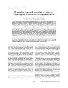
Figure 2: Expected power of visual test and the power of UMP test for sample size n = 100 and σ = 12.
B
●
● ●
16 40 20 0 −20 −40 A
17
18
19
●
● ● ●
●
● ●
● ●
B
A
●
B
●
● ● ● ●
●
A
B
A
Suppose each of N independent observers gives evaluations on multiple lineup plots and responses are associated with binary random variable Yij . Let Yij = 1, if subject j correctly identifies the test statistic on lineup i, and 0 otherwise. We model πij = E(Yij ) as a mixed effects logistic regression
20 ●
B
● ●
● ●
A
● ●
● ●
B
Xk
g(πij ) = Xij B + Zij τj (4) Figure 1: Lineup plot (m = 20) for testing H0 : βk = 0. When the alternative hypothesis is true the observed plot where τj is random effects coefficient vector of length q should show a vertical displacement between box plots. for subject j, τj ∼ M V N (0, Σ) with variance covariance matrix Σ, Zij is the ith row vector of random effects coCan you identify the observed plot? variates for subject j, B is a vector of coefficient of length p, the number of fixed effect covariates being used, Xij is uniform under H0 . In a lineup plot we simulate m − 1 the ith row vector of the fixed effects covariates for subject µ residual data sets from null model where each of these j and link function g(µ) = log( 1−µ ); 0 ≤ µ ≤ 1. The com−1 null data sets produces a corresponding p-value p0,i variates could be demographic information of people such and p0,i ∼ Uniform(0, 1) for i = 1, ..., m − 1. Suppose as age, gender, education level etc. as well as sample size p0 = mini (p0,i ). Thus p0 ∼ Beta(1, m − 1). (n), regression parameter (β) and variance (σ 2 ) of model Now assume that individuals pick the plot that has the 1. smallest p-value in the lineup plot. This leads to the de- From model 4 we obtain the power of the underlying testcision to reject H0 when pB < p0 . Thus we have the ing procedure as a population average for specified sample expected power as size (n) and variance (σ) as P ower(β) = P r(pB < p0 )
(2)
P ower(β) = π = P r(Y = 1|β, n, σ)
Figure 2 shows the power of UMP test and expected power of visual test obtained from equation (2). Notice that the expected power of visual test is almost as good as the power of UMP test. We estimate the empirical power from responses on a specific lineup plot generated with known values of sample size (n), variance (σ 2 ) and regression parameter (β) in model 1. Suppose, we have responses from N independent observers with u identifications of the observed plot. This gives an estimated power of P ower(β) =
u N
0≤u≤N
4
(5)
Simulation Experiment
The experiment is designed to study the ability of human observers to detect the effect of a single variable X2 (corresponding to parameter β2 ) in a two variable (p = 2) regression model (Equation (1)). Data is simulated for different values of β2 (= 0, 1, 3, 5, 7, 8, 10, 16), with two sample sizes (n = 100, 300) and two standard deviations of the error (σ = 5, 12). The set of β2 values was chosen so that estimates of the power should produce reasonable power curves, comparable to the theoretical UMP test. We
(3) 4
5
12
1.0 0.8 0.6 100
0.4
Power
0.2
test empirical
0.0
lower_limit
1.0
upper_limit UMP
0.8 0.6 300
0.4 0.2 0.0 −15
−10
−5
0
5
10
15
β
−15
−10
−5
0
5
10
15
Figure 3: Observed power of visual test from equation (3) with pointwise 95% confidence limits and the power of UMP test for sample size n = 100, 300 and σ = 12, 5. fixed the values of β0 = 5, β1 = 15 and values for X1 data sets were binned on this range by p-value, and a data were generated as a random sample from a Poisson(30) set was randomly selected from each bin. distribution. Data sets with different combinations of β2 , n and σ were generated with frequencies shown in Table 3. Three replicates of each level were generated. These Participants for the experiment were recruited through produced 60 different “observed data sets”. Amazon [2010] Amazon’s Mechanical Turk. Each participant was shown a sequence of 10 lineup plots. ParticiTable 3: Values of parameters considered for survey ex- pants are asked to select the plot with the biggest vertical difference, give a reason for their choice, and determine a periment level of confidence for their decision. Gender, age, educaSample size (n) σ values for β2 tion and geographic location of each participant are also 5 0, 1, 3, 5, 8 100 collected. In total, 3629 lineups were evaluated by 324 12 1, 3, 8, 10, 16 people coming from many different locations across the 5 0, 1, 2, 3, 5 globe. The results of the experiment are summarized in 300 12 1, 3, 5, 7, 10 Figure 3 which shows the observed power from the survey data calculated using equation (3) along with 95% confidence interval calculated using Fisher’s exact method. For added control, to ensure a signal in the simulated observed data a blocking structure was used to filter data sets. A 1000 sets were generated for each parameter combination and the traditional t-statistic and p-value associ- We fit model (4) to the survey data obtained from the simated with H0 : β2 = 0 were calculated. The 3 replicates ulation experiment. The estimated overall power curve were drawn from each of three blocks of p-values: (0.0- obtained from equation (5) is shown in Figure 4. Model q33 ), (q33 -q66 ), (q66 -1) where qi is the ith percentile in 4 also gives the subject specific power curves shown in the distribution of the p-values. Additional control was Figure 5. The plot includes 20 randomly selected subjectapplied to the 19 null plots. Because the distribution of specific power curves. Notice that the power curve estithese p-values should follow a Uniform(0,1) distribution, mated for one subject is above the UMP test power curve. 5
5
The purpose of this paper has been to examine the effectiveness of visual inference methods in direct comparison to existing inference methods. We need to be clear that this is not the purpose of visual inference generally: visual methods should not be seen as competitors to traditional inference. The purpose here, is to establish properties and efficacy of visual testing procedures in order to use them in situations where traditional tests cannot be used. For this experiment the effect of β2 was examined using sideby-side boxplots. Future experiments will be conducted to compare other regression parameters as described in Table 2 and assess sensitivity of power to modeling conditions.
0.8
Test
0.6
Power
empirical lower_limit upper_limit 0.4
UMP
0.2
−15
−10
−5
β
0
5
10
Conclusions
15
Acknowledgement: This work was funded by National Science Foundation grant DMS 1007697.
Figure 4: Estimated power curve from equation (5) along with 95% confidence interval for sample size n = 100 and σ = 12. The corresponding power curve for Uniformly Most powerful (UMP) test is shown for comparison.
References Amazon. Mechanical Turk, 2010. http://aws.amazon.com/mturk/.
URL
Andreas Buja, Dianne Cook, Heike Hofmann, Michael Lawrence, Eun-Kyung Lee, Deborah F. Swayne, and Hadley Wickham. Statistical inference for exploratory data analysis and model diagnostics. Royal Society Philosophical Transactions A, 367(1906):4361–4383, 2009. A. Gelman. Exploratory Data Analysis for Complex Models. Journal of Computational and Graphical Statistics, 13(4):755–779, 2004.
0.8
Hadley Wickham. ggplot2: Elegant graphics for data analysis. useR. Springer, 2009.
Power
0.6 gender Male Female
0.4
Leland Wilkinson. The Grammar of Graphics. Springer, New York, 1999.
0.2
−15
−10
−5
β
0
5
10
15
Figure 5: Estimated subject specific power curve from model 4 for sample size n = 100 and σ = 12. The corresponding power curve for Uniformly Most powerful (UMP) test is shown for comparison.
6
NY: