Statistical Learning Theory to Evaluate the Performance of Game ...

Statistical Learning Theory to Evaluate The Performance of Game Theoretic Power Control Algorithms for Wireless Data in Arbitrary Channels M. Hayajneh & C. T. Abdallah Dept. of Electrical & Computer Engr., Univ. of New Mexico,

EECE Bldg., Albuquerque, NM 87131-1356, USA. {hayajneh, chaouki}@ eece.unm.edu

Abstract—In this paper we use statistical learning theory to evaluate the performance of game theoretic power control algorithms for wireless data in arbitrary channels, i.e., no presumed channel model is required. To show the validity of statistical learning theory in this context, we studied a flat fading channel, and more specifically, we simulated the case of Rayleigh flat fading channel. With the help of a relatively small number of training samples, the results suggest the learnability of the utility function classes defined by changing the users power (adjusted parameter) for each user’s utility function.

I. I NTRODUCTION In game theoretic power control algorithms used in wireless code division multiple access (CDMA) cellular systems, the objective is to find the equilibrium power vector that maximizes the utility function of all users currently served in the cell [1][6]. The utility function quantifies the quality of service (QoS) obtained by a user in terms of the number of bits received correctly at the base station (BS) per one joule of power expanded [1]. The number of bits received correctly at the BS depends on the modulation scheme, coding, channel characteristics, etc. Unfortunately, most of the work on power control algorithms in wireless data CDMA cellular systems, has modelled the channel as an additive white Gaussian noise (AWGN) channel with deterministic channel gains [1]-[6]. Practically, the wireless data channel in CDMA cellular systems is a fading channel. In this paper we propose a distribution-free learning algorithm to evaluate the performance of game theoretic power control algorithms for wireless data in arbitrary channels, i.e, without prior knowledge of the channel model. It is very important in wireless data CDMA cellular systems to have a high signal-to-interference ratio (SIR), since this will result in very low error rate, a more reliable system, and a higher channel capacity, which means that more users can be served per cell [9]. It is however also important to lower the transmit power level, because low power levels result in longer batteries life and helps alleviate the near-far problem [12]. In this paper the original work in [1] is extended by considering more realistic channels benefiting from the ideas of distribution-free learning

theory. To show the validity of this technique we discuss in detail the application of distribution-free learning theory to a noncooperative power control game (NPG) and a noncooperative power control game with pricing (NPGP) under the assumption that the channel is modelled as a flat fading channel. The remaining of this paper is organized as follows: In section II we describe the utility function used in this paper, while in section III we present a discussion of two power control algorithms: NPG and NPGP. A brief discussion of distribution-free learning theory is presented in section IV. The application of distribution-free learning theory to NPG and NPGP under a flat fading channel model is introduced in section V. Discussion of a Rayleigh flat fading channel and simulation results are outlined in section VI. Finally, conclusions are presented in section VII. II. U TILITY F UNCTION Microeconomists use the concept of a utility function to quantify the level of satisfaction a player can get by choosing an action from its strategy profile given the other players’ actions. A utility function is chosen in such a way that puts all the elements of the game taking place between self-interested players in their most desired order. A formal definition of a utility function is available from [8]. Definition 1: Let A represent the set of all action sets that a player can choose, then the function u that evaluates numerically the elements of A such that u : A → R is called a utility function if for all a, b ∈ A, a player chooses the action set a rather than b if and only if u(a) ≥ u(b). It is known that in a cellular CDMA system there are a number of users sharing a spectrum and the air interface as common radio resources. Henceforth, each user’s transmission adds to the interference of all users at the receiver (BS). The objective of each user is to achieve a high quality of reception at the BS, i.e., a high SIR, by using the minimum possible amount of power to extend the battery’s life. Suppose we have a single-cell system with N users, where each user transmits packets of M total bits with L information bits and with power p Watts per bit. The rate of transmission is R bits/sec for all users. Let Pc (γ) represents the probability of correct reception of all bits in the frame at

0-7803-7701-X/03/$17.00 (C) 2003 IEEE

the BS at a given SIR γ. A suitable utility function for wireless data in CDMA system is then given by (see [1] and references therein): LR Pc (1) u= Mp u thus represents the number of information bits received successfully at the BS per joule of expanded energy. With the assumption of no error correction, perfect detection, and that each bit is experiencing independent noise, Pc is then given as
M M l=1 (1 − Pe (l)) , where Pe (l) is the lth bit error rate (BER) at a given SIR. III. P OWER C ONTROL A LGORITHMS FOR W IRELESS DATA The increase demand for handling information services within CDMA cellular systems increases the need for a new power control technology to improve the system performance, and to improve the efficiency of utilizing the shared radio resources by the different users currently served by the system. In this section, we review two power control algorithms that belong to a class of distributed asynchronous power control algorithms for wireless data: Non-cooperative power control game (NPG) and noncooperative power control game with pricing (NPGP). Both have already been studied in the literature [1]-[3] but we modify them in order to fit the fading channels that users experience in wireless data CDMA cellular systems. A. NPG Let N = {1, 2, ..., N } represent the index set of the users currently served in the cell and {Pj }j∈N represents the set of strategy spaces of all users in the cell. Let G = [N , {Pj }, {uj (.)}] denote a noncooperative game, where each user chooses its power level from a convex set Pj = [pj−min , pj−max ] and where pj−min and pj−max are the minimum and the maximum power levels in the jth user strategy space, respectively. With the assumption that the power vector p = [p1 , p2 , ..., pN ] is the result of NPG, the utility of user j is given as [1]: uj (p) = uj (pj , p−j )

(2)

where pj is the power transmitted by user j, and p−j is the vector of powers transmitted by all other users. The right side of (2) emphasizes the fact that user j can just control his own power and this will have great importance as we will see in section IV. We can rewrite (1) for user j as: uj (pj , p−j ) =

LR Pc (γj ) M pj

(3)

The formal expression for the NPG is given in [1] as: NPG :

max uj (pj , pj ), for all j ∈ N Pj

(4)

pj ∈

This game will continue to produce power vectors until it converges to a point where all users are satisfied with the utility level they obtained. This operating point is called Nash equilibrium point of NPG.

B. Nash Equilibrium in NPG The resulting power vector of NPG is called a Nash equilibrium power vector. Definition 2: [1] A power vector p = [p1 , p2 , ..., pN ] is a Nash equilibrium of the NPG defined above if for every j ∈   N , uj (pj , p−j ) ≥ uj (pj , p−j ) for all pj ∈ Pj . One interpretation of Nash equilibrium is that no user can increase its utility by changing its power level unilaterally. Sometimes, a user may find different values of transmit power levels from its strategy space that give the user similar values of the utility function for given power levels of the other users. For this reason, the best response correspondence rj (p−j ) was introduced [1]. It assigns to each p−j ∈ P−j the set rj (p−j )

=

  pj ∈ Pj : uj (pj , p−j ) ≥ uj (pj , p−j )   for all pj ∈ Pj

(5)

In light of this correspondence one can announce the power vector p = [p1 , p2 , ..., pN ] as a Nash equilibrium power vector if and only if pj ∈ rj (p−j ) for all j ∈ N . If we multiply the power vector p by a constant 0 < β < 1 we may get higher utilities for all users. This means that the Nash equilibrium is not efficient, that is, the resulting p is not the most desired social operating point. To obtain a Pareto dominant over pure NPG, NPGP was proposed in [1]. C. NPGP In NPGP, each user’s utility is the difference between its utility function defined under NPG and a pricing function. This allows us to use the system resources more efficiently, since each user is aware of the cost he/she incurs for aggressive use of the resources and of the harm he/she causes other users in the cell [1]. The pricing function discussed here is a linear pricing function, i.e., it is a pricing factor multiplied by the transmit power. This pricing factor is announced by the BS to the users currently in the cell in order to impose a Nash equilibrium that improves the sum of all utilities in the cell at lower power levels compared to the pure NPG [1]-[3]. In other words, the resulting power vector of NPGP is Pareto dominant [1] compared to the resulting power vector of NPG, but still not Pareto optimal in the sense that we can multiply the resulting power vector of NPGP by a constant 0 < β < 1 to obtain higher utilities for all users. Let us denote the N -player noncooperative power control game with pricing (NPGP) by Gc = [N , {Pj }, {ucj (.)}], where the utilities are given as [1]: ucj (p) = uj (p) − c pj for all j ∈ N

(6)

Where c is a positive scalar, chosen to get the best possible improvement in the performance. Therefore, NPGP with linear pricing function can be expressed as: NPGP : max {uj (p) − c pj } for all j ∈ N pj ∈Pj

0-7803-7701-X/03/$17.00 (C) 2003 IEEE

(7)

The question then becomes: does NPGP have a Nash equilibrium operating point similar to NPG?. In fact, the existence of Nash equilibria for NPG can be proved using analytical techniques because uj (p) is a quasiconcave utility function [1]. However, the utility function of NPGP (ucj (p)) is no longer quasiconcave which invalidates the analytical techniques used to prove the Nash existence for NPG. Fortunately, NPGP is a supermodular game [10] which has a Nash equilibria set Ec = [ps (c), pl (c)], where ps (c) and pl (c) are the smallest and the largest power vectors associated with pricing factor c, respectively [1]. More details about supermodular games and proofs are found in [1]. It should be noted here that for super2 modular games ∂ ∂P2cγ(γ) ≥ 0 must hold to guarantee the ex2

istence of a Nash equilibria set (Ec ). Suppose ∂ ∂P2cγ(γ) = 0 holds at γ = γ ∗ . The effect of this condition is that the strategy space (Pj ∀ j ∈ N ) must be modified to Pˆj = [p˜j , pj−max ] where p˜j leads to an SIR greater than γ ∗ for the jth user. Consider the asynchronous power control algorithm proposed in [1], which generates a sequence of power vectors that converges to the lowest power vector ps (c) in Ec . Assume user j updates its power level at time instances that belong to a set Tj , where tj 0 = 0 for Tj = {tj 1 , tj 2 , ...}, with tj k < tj k+1 and   all j ∈ N . Let T = {t1 , t2 , ...} where T = T1 T2 ... TN with tk < tk+1 and define p to be the smallest power vector in ˆ We then use the following algothe modified strategy space P. rithm to find a Nash equilibrium point of NPG (c = 0) and of NPGP (c = 0). Algorithm 1: [1] Consider NPGP as given in (7) and generate a sequence of power vectors as follows: 1) Set the power vector at time t = 0: p(0) = p, let k = 1 2) For all j ∈ N , such that tk ∈ Tj : a) Given p(tk−1 ), calculate rj (tk )= arg maxˆ ucj (pj , p−j (tk−1 )) pj ∈ Pj b) Let the transmit power pj (tk ) = min(rj (tk )) 3) If p(tk ) = p(tk−1 ) stop and declare the Nash equilibrium power vector as p(tk ), else let k := k + 1 and go to 2. The following algorithm is to find the best pricing factor c: Algorithm 2: 1) Set c = 0 and announce c to all users currently in the cell. 2) Use Algorithm1 to obtain ucj for all j ∈ N at equilibrium. 3) Increment c := c + ∆c, ∆c is a positive constant, and announce c to all users, and then go to 2. 4) If ujc+∆c ≥ ucj for all j ∈ N go to 3, else stop and declare the best c. In the next section we present a brief discussion of distributionfree learning theory, where we focus on the learnability of the utility function class, depending on learning samples received at the BS. IV. D ISTRIBUTION -F REE L EARNING Distribution-free learning theory enables us to evaluate the performance of a game theoretic power control algorithms for

wireless data without the need to know the channel model a priory. Of course, this only can be done under the condition that the utility function class is learnable. Learnability of the utility function class highly dependent on the channel model as will be apparent shortly. If a function (concept) class has a finite P -dimension ( VCdimension), then such function (concept) class is said to be a distribution-free learnable [13], that is we can learn the target function (concept) using the learning samples drawn according to an unknown probability measure. The learning problem under study is as follows: assume (X, S) is a given measurable space (S is σ-algebra of subsets of X), and U (utility function class) is a family of measurable functions such that u : X → [0, 1] ∀u ∈ U. It should be noted here that the interval [0, 1] does not necessarily mean that the function u ∈ [0, 1], but rather that it is bounded [14]. Suppose P represents the set of all probability measures on (X, S). For a given function u ∈ U, a probability measure P ∈ P, and a learning multisample x = [x1 , x2 , ..., xn ] ∈ X n . Then the average utility function U is given by: U

:= :=

EP (u)  u(x)dP (x) X

(8)

while the empirical utility function Uemp is given by: Uemp := n−1

n 

u(xl )

(9)

l=1

For " > 0, define δ(n, ", P ) as follows [13]:   n n x ∈ X : sup |Uemp − U | > " δ(n, ", P ) := P

(10)

u∈U

where P n denotes the n-manifold probability measure on X n , and define δopt (", n) := sup δ(n, ", P ) P ∈P

The family of function classes U has the property of distribution-free uniform convergence of empirical means if δopt (n, ") → 0 as n → ∞ for each " > 0 [13]. Which is a result of the following theorem stated without proof, which may be found in [13]. Theorem 1: [13] Suppose the family U has a finite Pdimension with value equal to d. Consider 0 < " < e/(2 log2 e) ≈ 0.94. Then δopt (n, ") ≤ 8



16e 16e ln " "

d

exp(−n"2 /32) ∀n

Therefore U has the property of distribution-free uniform convergence of empirical means. One can see from the above theorem that the learnability of U is highly dependent on the P-dimension (d) for a given accuracy ("), where a large value of d could lead to a prohibitive sample complexity (n) to achieve the accuracy with confidence

0-7803-7701-X/03/$17.00 (C) 2003 IEEE

δopt (n, "). In the next section we study the learnability of the utility function class defined under NPG and NPGP by evaluating the P-dimension with the assumption that the channel is modelled as a flat fading channel.

Notice that ui = LMR f4 . Now, we need to find the first-order partial derivative of {fk } with respect to pi and αi in order to show the learnability of ui in (13). ∂f1 ∂αi

V. A PPLICATION TO NPG AND NPGP IN A F LAT FADING C HANNEL

=

In this section we apply distribution-free learning theory where the channel is modelled as a flat fading channel. Using this model, the SIR (γi ) of the ith user is given by [11]: pi hi αi2 W γi = N R k=i pk hk αk2 + σ 2

∂f1 ∂pi

Cγi

(11) ∂f2 ∂αi

∂f2 ∂pi

Where Pe was replaced by 2Pe to give the utility function (ui ) this property: ui → 0 as pi → 0 and ui → 0 as pi → ∞ [1]. Let us split up the ith utility function into the following functions ∀i ∈ N : f1 = 1 − e

−γi /2

,

(14)

f2 =

f1M ,

(15)

f3 =

1 , pi

(16)

f4 =

f2 f3

(17)

and finally

∂f1 ∂γi ∂γi ∂pi 1 1 (− f1 + )(Cγi αi2 ) 2 2

=

1 1 = M f1M −1 (− f1 + )(Cγi αi2 ) 2 2

=

(20)

(21)

= 0

(22)

= −f32

(23)

∂f2 ∂f3 − f2 ∂α f3 ∂α i i

f32

= M f1M −1 (−f1 + 1)(Cγi p2i αi ) ∂f4 ∂pi

(19)

∂f2 ∂f1 ∂f1 ∂pi

∂f3 ∂pi ∂f4 ∂αi

(18)

∂f2 ∂f1 ∂f1 ∂αi

∂f3 ∂αi

A simple interpretation of (12) is that the interference and the background noise are considered constant at each time instance the user adjusts its power (see algorithm 1). Suppose that each user is using noncoherent binary shift keying (BFSK) to transmit each data bit, i.e, Pe = 12 e−γ/2 . The channel is assumed to be a slow flat fading channel, in other words, the fading coefficient αi is constant for each frame time interval. This enables us to write Pc (γi ) = (1 − Pe (γi ))M . So, we can rewrite (1) for the ith user in the following form: (13)

=

∂f1 ∂γi ∂γi ∂αi (−f1 + 1)(Cγi pi αi )

= M f1M −1 (−f1 + 1)(Cγi pi αi )

hi W = N R k=i pk hk αk2 + σ 2

LR ui = (1 − e−γi /2 )M M pi

= =

where W is the spread-spectrum bandwidth, R is the data rate (bits/sec), pk is the transmitted power (the adjusted parameter) of the kth user, hk is the path gain between the BS and the kth user, σ 2 is the variance of the AWGN channel, and αk is a flat fading coefficient of the path between the BS and kth user. For both NPG and NPGP, it is assumed that each user knows the background noise and the interference from other users at each time instance he updates his transmit power level. This allows the user to adjust his own parameter (power) to obtain the maximum possible utility function. This then enables us to write (11) in the form: (12) γi = Cγi pi αi2 , where

=

=

(24)

∂f3 2 f3 ∂f ∂pi − f2 ∂pi

f32

1 1 = M f1M −1 (− f1 + ) 2 2 × (2Cγi pi αi2 + p2i f2 f32 )

(25)

As we can see from the above first-order partial derivatives that f1 , f2 , f3 , f4 are a Pfaffian chain of length q = 4 and of degree at most D = 3 in αi and pi . The importance of this observation is in the following result ([13], Theorem 10.8): d

≤ 2l(l(q + 1)2 /2 + log2 d + (2(q + 1) + 1) log2 l +

(q + 2) log2 (2(d + D)) + log2 (2e))

(26)

Where d is the P -dimension of the function class U, l is the number of adjustable parameters of each user (in the case under study the parameters are pi and Cγi , that is l = 2). Substituting the numerical values of D, q, and l, we get d ≤ 247. These results can be extended to NPGP in a straight forward lending to get the same values of D, q and l. Henceforth, utility function classes defined under NPG and under NPGP have the same upper bound on the P -dimension.

0-7803-7701-X/03/$17.00 (C) 2003 IEEE

VI. D ISCUSSION OF R AYLEIGH F LAT FADING C HANNEL AND S IMULATION R ESULTS As a specific case of flat-fading channel model we present results for the case where αi is modelled as a Rayleigh random variable with a probability distribution given by: p(αi ) = σr2

αi exp(−αi2 /2σr2 ), σr2

i = 1, 2, ..., N

respect to xi . Since αi is Rayleigh distributed random variable, then αi2 is exponentially distributed with mean equal to 1. Therefore, µxi the mean of xi is given as:

µxi

(27) =

E{αi2 }/2

Where = is the measure of the spread of the distribution. In the following calculations it was assumed that σr2 = 1/2. For simplicity let us express the interference from all other users as xi , i.e. xi =

N 

pk hk αk2

(28)

k=i

therefore (11) can be written as: γi

=

W pi h i α2 R xi + σ 2 i

LR (1 − e−γi /2 )M M pi

(30)

and ui (p/xi ) is given by:

0



∞

ui (p/γi , xi ) p(γi /xi ) dγi

∞

LR 1 γi (1 − e−γi /2 )M  exp(−  ) dγi M pi γi γi 0

M M LR  = (−1)k  k M pi γi k=0

 ∞ 1 k × exp −( +  ) γi dγi 2 γi 0

M L R  M 2 (−1)k (32) =  k k γi + 2 M pi k=0 =

k=i

pk hk E{αk2 }



pk h k

(34)

k=i

Henceforth, the average utility function of the ith user is given by: LR M pi

γi =

Using (29) and (27) the distribution of γi for fixed xi is given as: 1 γi p(γi /xi ) =  exp(−  ) (31) γi γi 

N 

αk2 pk hk



M 1  M 2 (−1)k 1+ k γi k k=1

(35)

(29)

In this context (13) should be written as:

=

=



 

where γi is the average SIR given by:



ui (p/xi )

N  k=i

Ui (p) =

= γi αi2

ui (p/γi , xi ) =

= E{xi } = E

 N 



For high SIR (γi  1) (32) can be approximated by



M LR 1  M 2 (−1)k u(p/xi ) ≈ 1+  k M pi k γi

(33)

k=1

To complete the derivation of average utility function of the ith user Ui (p), we only need to find the expectation of (33) with

pi h i W  2 R N k=i pk hk + σ

(36)

While the empirical value of the utility function Uempi is given by: n  Uempi = n−1 ui (ˇ αl ), (37) l=1

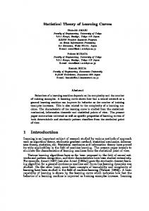
where α ˇ = [α1 , α2 , ..., αN ]. The system studied is a singlecell with 9 stationary users (N = 9) using the same data rate R and the same modulation scheme, noncoherent BFSK. The system parameters used in this study are given in Table I. The distances between the 9 users and the BS are d = [310, 460, 570, 660, 740, 810, 880, 940, 1000]. The path attenuation between user j and the BS using the simple path loss model [12] is hj = 0.097/d4j . Using (26) and theorem 1 with accuracy " = 0.94 and confidence 1 − δopt (", n) ≈ 0.99 (see theorem 1 for the definition of δopt (", n) ) the sample complexity required was n ≤ 47000. Fig.1 and Fig.2 show, respectively, the equilibrium utilities and the equilibrium powers (o) obtained by NPG using the average utility function in (35) compared to the empirical values obtained by simulating the Rayleigh flat fading channel (+). In the simulation, the sample complexity (the number of samples drawn from the channel according to a Rayleigh distribution) was 47, 000 as mentioned above. NPG was run for each sample from the channel, then the empirical means of the equilibrium utilities were calculated according to (37). As one can see, the figures show that the empirical results (+) fit the results obtained by averaging with respect to the known distribution (Rayleigh distribution in our case) (o). This proves the learnability of the utility function classes U with reasonable sample complexity.

0-7803-7701-X/03/$17.00 (C) 2003 IEEE

TABLE I THE VALUES OF PARAMETERS USED IN THE SIMULATIONS .

L, number of information bits 64 M length of the codeword 80 W , spread spectrum bandwidth 107 Hz R, data rate 104 bits/sec 2 σ , AWGN power at the BS 5 × 10−15 N , number of users in the cell 9 W/R, spreading gain 1000

[9] J. Zander. “Distributed cochannel interference control in cellular radio systems,”IEEE Tran. Veh. Tchnol., VOL. 41, pp. 305- 311, Aug. 1992. [10] D. M. Topiks, “Equilibrium points in nonzero n-person supermodular games,”SIAM Control and Optimization, VOL. 17, NO. 6, pp. 773-787, 1979. [11] J. G. Proakis, Digital Communications, The McGraw Hill Press 1221 Avenue of the Americas, New York, NY 10020, 2000. [12] Roger L. Peterson, Rodger E. Ziemer and David E. Borth, Introduction to Spread Spectrum Communications, Prentice Hall, Upper Saddle River, NJ 07458, 1995. [13] M. Vidyasagar, A Theory of Learning and Generalization with Applications to Neural Networks and Control Systems. Berlin, Germany: Springer-Verlag, 1996. [14] Simon Haykin, Neural Networks A Comprehensive Foundation, Prentice Hall, Upper Saddle River, NJ 07458, 1994.

VII. C ONCLUSIONS 8

10

average empirical

equilibrium utilities (bits/Joul)

We studied a noncooperative power control game (NPG) and noncooperative power control game with pricing (NPGP) introduced in [1]-[3] using more realistic channels as in [7]. We proposed the use of distribution-free learning theory to evaluate the performance of game theoretic power control algorithms for wireless data CDMA cellular systems in arbitrary channels. We studied in detail the case when the channel is modelled as a flat fading channel. We evaluated an upper bound for the Pdimension of the utility function class and we presented a simulation results for the Rayleigh case, which showed the learnability of the utility class function defined by adjusting the power for each user. We are currently studying the application of distribution-free learning theory to a frequency and a time selective fading channels.

7

10

6

10

3

10 distance between BS and terminal (meters)

Fig. 1. Equilibrium utilities of NPG for Rayleigh flat fading channel by using (35) (o) and by simulation with samples drawn according to Rayleigh distribution (+) versus the distance of a user from the BS in meters with W/R = 1000.

R EFERENCES average empirical

−3

10

equilibrium powers (Watts)

[1] C. U. Saraydar, N. B. Mandayam, and D. J. Goodman, “Efficient power control via pricing in wireless data networks.”, IEEE Tras. Comm., VOL. 50, NO. 2, pp. 291- 303, Feb. 2002 [2] N. Shah, N. B. Mandayam, and D. J. Goodman. “Power control for wireless data based on utility and pricing.” In Proceedings of PIMRC, pp. 1427-1432, 1998. IEEE Trans. Vehic. Tech., 41(3):305-311, Aug. 1992. [3] C. U. Saraydar, N. B. Mandayam, and D. J. Goodman, “Pricing and power control in multicell wireless data network,” IEEE JSAC, VOL. 19, NO. 10, pp. 1883- 1892, Oct. 2001 [4] D. Goodman and M. Mandayam, “Power control for wireless data,”in IEEE International Workshop on Mobile Multimedia Communications, 1999, pp. 55-63. [5] Allen B. Mackenzie and Stephen B. Wicker, “Game theory and the design of self-configuring, adaptive wireless networks,” IEEE Communications Magazine, VOL. 39 Issue: 11 , Nov. 2001 pp. 126 -131. [6] Allen B. Mackenzie and Stephen B. Wicker, “Game theory in communications: motivation, explanation, and application to power control ,”IEEE Global Telecommunications Conference, 2001, VOL. 2, pp. 821 -826 [7] P. Ligdas and N. Farvardin, ”Finite-State Power Control for Fading Channels,” Proc. Conference on Information Sciences and Systems, Johns Hopkins University, Baltimore, MD, March, 1997 [8] D. Fudenberg and J. Tirole. Game Theory, The MIT Press, 1991.

−4

10

3

10 distance between BS and terminal (meters)

Fig. 2. Equilibrium powers of NPG for Rayleigh flat fading channel by using (35) (o) and by simulation with samples drawn according to Rayleigh distribution (+) versus the distance of a user from the BS in meters with W/R = 1000.

0-7803-7701-X/03/$17.00 (C) 2003 IEEE