A new linearization model with density response based on information ... proposed for the prediction of dynamic response of a stochastic nonlinear system.
R. J. Chang Professor
S. J. Lin
Statistical Linearization Model for the Response Prediction of Nonlinear Stochastic Systems Through Information Closure Method
Graduate Student Department of Mechanical Engineering, National Cheng Kung University, 701 Tainan, Taiwan, R.O.C.
1
A new linearization model with density response based on information closure scheme is proposed for the prediction of dynamic response of a stochastic nonlinear system. Firstly, both probability density function and maximum entropy of a nonlinear stochastic system are estimated under the available information about the moment response of the system. With the estimated entropy and property of entropy stability, a robust stability boundary of the nonlinear stochastic system is predicted. Next, for the prediction of response statistics, a statistical linearization model is constructed with the estimated density function through a priori information of moments from statistical data. For the accurate prediction of the system response, the excitation intensity of the linearization model is adjusted such that the response of maximum entropy is invariant in the linearization model. Finally, the performance of the present linearization model is compared and supported by employing two examples with exact solutions, Monte Carlo simulations, and Gaussian linearization method. 关DOI: 10.1115/1.1688762兴
Introduction
The prediction of the dynamic behavior of nonlinear stochastic systems is an important research topic in the areas of system dynamics and control engineering 关1–3兴. For the prediction of the system response, a solvable dynamic model for describing the dynamic behavior of a stochastic system is usually required. When a nonlinear stochastic dynamic system is described by employing Ito’s differential equation, the dynamic response can be completely characterized by the associated Fokker-PlanckKolmogorov 共FPK兲 equation. However, except for very limited cases, it is usually very difficult to solve the FPK equation analytically 关1,2兴. Some approximate analytical and numerical methods are usually employed for solving the response statistics through the FPK equation 关1– 4兴. Although many approximate analytical schemes have been developed for solving the stochastic response, a statistical linearization scheme is still one of the most effective methods employed for predicting the response of general nonlinear systems 关5兴. For effectively predicting the dynamic behavior of nonlinear stochastic systems, different linearization models have been extended from stationary methods for obtaining non-stationary response 关5–10兴. In employing these linearization techniques, two important issues concerning the accuracy of moment response and the applicable stability boundary need to be investigated 关5兴. The development of Gaussian linearization model is one of the most widely used techniques for predicting dynamic behavior. The predicted accuracy by the Gaussian linearization method is quite acceptable for weakly nonlinear systems, but for strongly nonlinear systems the errors in the predicted moments may be up to several ten percentages 关11兴. For improving the accuracy predicted by the Gaussian linearization model, many different approaches have been proposed by utilizing non-Gaussian linearization techniques 关8 –10兴. Although some improvements in predicting moment response have been reported, in general, the error bounds in the Contributed by the Technical Committee on Vibration and Sound for publication in the JOURNAL OF VIBRATION AND ACOUSTICS. Manuscript received August 2002; Revised November 2003. Associate Editor: L. A. Bergman.
438 Õ Vol. 126, JULY 2004
predicted response cannot be certainly guaranteed by these nonGaussian techniques. In addition, the applicable stability boundary in utilizing the non-Gaussian linearization techniques is still unknown 关11兴. The analysis of stochastic dynamics from the viewpoint of information theory is gaining notice in the recent researches 关12– 18兴. Different maximum entropy schemes were developed to analyze the stationary and non-stationary responses of stochastic dynamic systems. Haken 关12兴 used the maximum entropy principle to solve the dynamic transition around the stationary states. Chang 关13兴 developed an analytical scheme through perturbation in maximum entropy for analyzing the response of a stochastic parametrically excited system. Sobczyk and Trebicki 关14,15兴 proposed a numerical scheme based on the maximum entropy principle for obtaining the non-stationary response of stochastic systems. Jumarie 关16兴 formulated a non-stationary solution of FPK equation by utilizing maximum path entropy. Phillis 关17兴 extended the stability criterion for stochastic evolution in the entropy sense. Recently, Chang and Lin 关18兴 developed an information closure method for the robust prediction of stability boundary of a nonlinear stochastic system. Although different entropy schemes have been employed for analyzing the dynamics of a nonlinear stochastic system, an effective method for predicting the response of a general state equation of a nonlinear stochastic system has not been fully developed. In this paper, a new statistical linearization model based on the information closure scheme 关18兴 is developed for the accurate prediction of statistical response of a nonlinear stochastic system. For the development of the linearization model, an information closure scheme is first employed for stability analysis under the information of moment constraint. Under the constrained information, both the density function and maximum entropy are estimated by the maximum entropy principle. For the prediction of moment response of a nonlinear stochastic system, an information-closure statistical linearization model is constructed by utilizing the estimated density function. In addition, the intensity of excited noise of the linearization model is adjusted according to the estimated maximum entropy. The applications of the
Copyright © 2004 by ASME
Transactions of the ASME
Downloaded From: http://computationalnonlinear.asmedigitalcollection.asme.org/ on 03/24/2015 Terms of Use: http://asme.org/terms
present linearization model for the accurate prediction of statistical response under robust stability boundary are illustrated by selecting two nonlinear stochastic systems under the a priori constraints of moment information.
scheme. After the equivalent linear model is developed, the dynamics of the nonlinear stochastic systems can be predicted effectively.
3 2 Dynamic Formulations and A Priori Moment Information Consider a general n-dimensional nonlinear Ito’s stochastic system that is derived from replacing the physical white noise by an ideal one through incorporating Wong-Zakai correction terms and described as dX 共 t 兲 ⫽F 共 X 共 t 兲 ,t 兲 dt⫹G 共 X 共 t 兲 ,t 兲 dW 共 t 兲 X 共 t 0 兲 ⫽X 共 0 兲
(1)
where X(t) is an n⫻1 vector of state processes, X(0) is an initial condition with given distribution, F(X(t),t) is an n⫻1 vector, in general, to be expressed as a polynomial-type nonlinear function of states, G(X(t),t) is an n⫻m matrix to be expressed as a polynomial-type nonlinear function of states, F(X(t),t) and G(X(t),t) satisfy the uniform Lispschitz and uniform growth conditions, and W(t) represents a zero-mean m⫻1 vector Wiener process with intensity E 关 dW 共 t 兲 dW T 共 t 兲兴 ⫽Q w 共 t 兲 dt.
(2)
The statistical information provided by the dynamic system 共1兲 is completely characterized by a probability density function which is governed by the FPK equation. The statistical information characterized by the FPK equation can be expressed through the nonstationary response governed by the following moment propagation equations d E 关 w K 共 X 兲兴 ⫽E dt
冋兺 n
f i共 X 兲
i⫽1
1 ⫹ 2
n
n
兺兺
i⫽1 j⫽1
w K共 X 兲 xi 2w K共 X 兲 共 G 共 X 兲 Q w共 t 兲 G 共 X 兲 T 兲 i j x i x j
⫽E 关 K 共 X 兲兴 where
k k k w K (X)⫽x 11 x 22 ¯x nn ,
K共 X 兲 ⫽
兺
册
H 共 t 兲 ⫽⫺
k 1 ,k 2 ,¯ ,k n
k
k
k
c k 1 k 2 ¯k n x 11 x 22 ¯x nn ,
l
⬁
⫺⬁
冕
⬁
⫺⬁
p 共 X,t 兲 ln p 共 X,t 兲 dX.
p 共 X,t 兲 dX⫽1.
˜ 共 t 兲 ⫽⫺ H ⫺
冕
⬁
⫺⬁
兺 L
p 共 X,t 兲 ln p 共 X,t 兲 dX⫺ ⬘0 共 t 兲
L共 t 兲
冋冕
⬁
⫺⬁
(7)
冋冕
⬁
⫺⬁
p 共 X,t 兲 dX⫺1
w L 共 X 兲 p 共 X,t 兲 dX⫺a L 共 t 兲
册
册
(8)
where ⬘0 (t)苸R and L (t)苸R are undetermined Lagrange multipliers at each time instant. To maximize the entropy functional, one performs ˜ 共t兲 ␦H ⫽0. ␦p
(9)
The estimated quasi-stationary probability density becomes
冉 冉
p 共 X,t 兲 ⫽exp ⫺1⫺ ⬘0 共 t 兲 ⫺ ⫽exp ⫺ 0 共 t 兲 ⫺
(5)
(6)
By introducing the Lagrange multipliers, the entropy functional can be constructed as
(4)
with w L (X)⫽x 11 x 22 ¯x nn , l i ⭓0, i⫽1⬃n and a L (t) as a priori moment information at each time instant. Here, it is noticed that for the nonlinear stochastic system, the moment information can be available from experiments, Monte Carlo simulations, or moment equations in 共3兲. For the development of a statistical linearization model applicable under the stability boundary, a new linearization formulation is to replace the nonlinear functions in 共1兲 by linear ones with the linearization coefficients obtained through the information closure Journal of Vibration and Acoustics
冕
In Eq. 共6兲, the evolution of entropy process H(t) is assumed to be slower than the dynamic evolution of stochastic fluctuation of the system by Eq. 共3兲. Next, by employing Jaynes’ maximum entropy principle, p(X,t) can be derived at each time instant such that the entropy by equation 共6兲 can be maximized under the constraints of 共5兲 and with the normalization condition
k i ⭓0, i⫽1⬃n,
E 关 w L 共 X 兲兴 ⫽a L 共 t 兲 l
3.1 Information Closure and Maximum Entropy Estimation. By following the information closure scheme 关18兴, firstly, the Shannon’s entropy can be defined and extended to a quasistationary process as
(3)
and f i (X) is the ith component of F(X(t),t). The moment equations from 共3兲 generally are not in closure but with infinite hierarchy. Also, the density functions in general are hardly to be solved from the FPK equation. For analyzing the dynamics of the general nonlinear stochastic system 共1兲, the information closure scheme 关18兴 based on Jaynes’ maximum entropy principle 关19兴 is first utilized for the closure of the infinite hierarchy of moment equations. For the general stochastic system described by equations 共1兲 and 共2兲, a priori information about the system at each time instant is to be given through moments as
l
Information Closure Scheme
兺 共 t 兲w 共 X 兲 L
L
L
兺 共 t 兲w 共 X 兲 L
L
L
冊
冊
(10)
with 0 (t)⫽1⫹ 0⬘ (t). With the density function, the maximum entropy evolved at each time instant can be estimated by H 共 t 兲 ⫽ 0 共 t 兲 ⫹ with E 关 w L 共 X 兲兴 ⫽
兺 共 t 兲 E 关 w 共 X 兲兴 L
L
冕
⬁
⫺⬁
⫺
(11)
L
冉
w L 共 X 兲 exp ⫺ 0 共 t 兲
兺 M
M共 t 兲w M共 X 兲
冊
dX.
3.2 Accurate Response Analysis. For the accurate analysis of dynamic response by the present scheme, a set of equations with undetermined Lagrange multipliers needs to be formulated. By substituting the density function 共10兲 into 共5兲, one has
冕
⬁
⫺⬁
冉
w L 共 X 兲 exp ⫺ 0 共 t 兲 ⫺
兺 M
M共 t 兲w M共 X 兲
冊
dX⫽a L 共 t 兲 . (12)
From Eq. 共12兲, the Lagrange multipliers can be solved in each time instant. If an exact moment information is not available, however, the equivalent information can be employed from the JULY 2004, Vol. 126 Õ 439
Downloaded From: http://computationalnonlinear.asmedigitalcollection.asme.org/ on 03/24/2015 Terms of Use: http://asme.org/terms
moment equation 共3兲. By substituting the density function 共10兲 into 共3兲 and utilizing the time derivative of the normalization condition 共7兲, the set of equations with undetermined Lagrange multipliers 共13a兲 and 共13b兲 can be obtained, respectively as ⫺˙ 0 共 t 兲 E 关 w K 共 X 兲兴 ⫺
兺
˙ L 共 t 兲 E 关 w K⫹L 共 X 兲兴 ⫽E 关 K 共 X 兲兴
L
(13a) and
兺 ˙ 共 t 兲 E 关 w 兴 ⫽0
⫺˙ 0 共 t 兲 ⫺ with E 关 w K 共 X 兲兴 ⫽
冕
⬁
k
⫺⬁
⫻
冉兿
冕
⬁
⫺⬁
⫻
k
k
冊
冉兿
冉兿 L
c k 1 k 2 ¯k n
冕
⫽
兺
k 1 ,k 2 ,¯k n
⫻
冉兿 L
冕
⫺⬁
k
li i,l 共 t 兲 x i
冊
li i,l 共 t 兲 exp共 ⫺ i,l 共 t 兲 x i 兲
(16) n
and
the
normalization
constants
satisfy
兿 N i,l (t)⫽exp
k
k
(⫺0,l (t)). By employing 共15兲 and 共16兲, the estimated system entropy 共11兲 at each time instant can be derived as
k
x 11 x 22 ¯x nn
冊
n
H l 共 t 兲 ⫽ 0,l 共 t 兲 ⫹
k
x 11 x 22 ¯x nn
兺 i⫽1
li i,l 共 t 兲 E 关 x i 兴
(17)
⬁ with E 关 x i i 兴 ⫽N i,l (t) 兰 ⫺⬁ x i i exp(⫺i,l(t)xii)dxi . Now, the system entropy 共17兲 and the associated density function 共16兲 are expressed explicitly in terms of the Lagrange multipliers. The Lagrange multipliers satisfy a set of equations obtained by substituting 共16兲 into 共13兲 to give l
l
l
n
⫺˙ 0,l 共 t 兲 E 关 w K 共 X 兲兴 ⫺
兺 ˙ i⫽1
li i,l 共 t 兲 E 关 w K 共 X 兲 x i 兴 ⫽E 关 K 共 X 兲兴
(18a) and n
⫺˙ 0,l 共 t 兲 ⫺
兺 ˙ i⫽1
li i,l 共 t 兲 E 关 x i 兴 ⫽0
(18b)
with
冊
n
E 关 w K 共 X 兲兴 ⫽
N L 共 t 0 兲 exp共 ⫺ L 共 t 0 兲 w L 共 X 兲兲 dX.
In using the information closure scheme, more accurate density function can be obtained if more a priori information of the moments 共5兲 are available. When the given a priori information of moments is accurate, the entropy estimated by the closure scheme is guaranteed to give the upper bound of the true system entropy. When the density associated with the upper bound of entropy is estimated, the estimated density can be directly employed for robust analysis of the system stability. 3.3 Robust Stability Analysis. In developing a robust stability analysis, the accuracy of estimated density is not of real concern as in the accurate response analysis 关18兴. By employing the information closure method for robust analysis, all of the in-
兿
i⫽1
冉 冕 N i,l 共 t 兲
⬁
k
⫺⬁
l
x i i exp共 ⫺ i,l 共 t 兲 x i i 兲 dx i
冊
n
(14)
440 Õ Vol. 126, JULY 2004
i⫽1
i⫽1 ⬁
⫺⬁
k
兿N i⫽1
In the selection of moments for the information constraints by w L (X) in above equations, every dimension of states x i must be selected for the n-dimensional system 共1兲. That is, all of the l i in w L (X) must not be zero for each information constraint. Specifically, if the constraints 共5兲 are selected such that only the secondorder terms are retained in w L (X), the general non-Gaussian information closure scheme becomes a Gaussian closure one. However, the w K (X) in moment equation 共3兲 must be suitably selected so that there is one unique solution in the set of differential equation 共13兲. The selection of w K (X) can be searched sequentially from the low order moment equations to the higher ones. For the given initial moment information as E 关 w K (X(t 0 )) 兴 , the initial conditions L (t 0 ) can be determined from the normalization condition 共7兲 and the moment equation 共3兲 to yield E 关 w K 共 X 共 t 0 兲兲兴 ⫽
兺
n
N L 共 t 兲 exp共 ⫺ L 共 t 兲 w L 共 X 兲兲 dX.
⬁
n
p l 共 X,t 兲 ⫽exp ⫺ 0,l 共 t 兲 ⫺
冊
兺
(15)
is selected and employed as a set of constraints in the information closure scheme. The selection of w L (X) for the robust stability analysis is different from that for the accurate response analysis. According to the maximum entropy principle, the estimated entropy through 共15兲 will larger than that with multi-modes with or without interaction modes in 共5兲. As far as the available information of single modes is sufficient, the maximum entropy estimated is guaranteed to give the upper bound of the true system entropy. Moreover, the parametric studies on density, and entropy evolution by Eqs. 共10兲, and 共11兲, respectively can be undertaken by employing the single modes w l (x i ) in 共15兲. By employing Eq. 共15兲 in the density function 共10兲, the quasistationary probability density is expressed as
N L 共 t 兲 exp共 ⫺ L 共 t 兲 w L 共 X 兲兲 dX,
k 1 ,k 2 ,¯ ,k n
with l i ⬎0,i⫽1⬃n,
冉
N L 共 t 兲 exp共 ⫺ L 共 t 兲 w L 共 X 兲兲 dX,
and
⫻
l
w l 共 x i 兲 ⫽x i i
k ⫹l k ⫹l k ⫹l x 11 1 x 22 2 ¯x nn n
L
E 关 K 共 X 兲兴 ⫽
(13b)
L
x 11 x 22 ¯x nn
L
E 关 w K⫹L 共 X 兲兴 ⫽
L
L
teraction modes of states can be ignored in the formulation. Instead of utilizing 共12兲, all available w L (X) are separated and decoupled in each state. Only one single mode in each state as
⫽
兿 2N i⫽1
⫺1 ⫺ 共 k i ⫹1 兲 /l i 共 t 兲 ⌫ 共共 k i ⫹1 兲 /l i 兲 , i,l 共 t 兲 l i i,l
(18c) n
l
E 关 w K共 X 兲 x ii 兴 ⫽
兿
i⫽1
冉
N i,l 共 t 兲
冕
⬁
⫺⬁
k ⫹l i
xi i
l
exp共 ⫺ i,l 共 t 兲 x i i 兲 dx i
冊
n
⫽
兿 2N i⫽1
⫺1 ⫺ 共 k i ⫹l i ⫹1 兲 /l i 共 t 兲 ⌫ 共共 k i ⫹l i ⫹1 兲 /l i 兲 , i,l 共 t 兲 l i i,l
(18d) and Transactions of the ASME
Downloaded From: http://computationalnonlinear.asmedigitalcollection.asme.org/ on 03/24/2015 Terms of Use: http://asme.org/terms
E 关 K 共 X 兲兴 ⫽
兺
k 1 ,k 2 ,¯ ,k n
冉
n
⫻
兿
i⫽1
N i,l 共 t 兲
冕
⬁
k
⫺⬁
l
x i i exp共 ⫺ i,l 共 t 兲 x i i 兲 dx i
冉兿
冊
n
兺
⫽
c k 1 k 2 ¯k n
k 1 ,k 2 ,¯ ,k n
c k 1 k 2 ¯k n
⫻⌫ 共共 K i ⫹1 兲 /l i 兲
冊
i⫽1
⫺ 共 k i ⫹1 兲 /l i
2N i,l 共 t 兲 l i⫺1 i,l
共t兲
(18e)
where ⌫共•兲 represents a gamma function and the expected values in 共18兲 are non-zero for even function. By employing the closure scheme in stationary, the probability density function 共16兲 becomes
冉
n
p l 共 X 兲 ⫽exp ⫺ 0,l ⫺
兺
i⫽1
l
冊
兿
l
i⫽1
N i,l exp共 ⫺ i,l x i i 兲 . (19)
The differential equations of Lagrange multipliers 共18兲 become the algebraic equations as E 关 k 共 X 兲兴 ⫽
兺
k 1 ,k 2 ,¯ ,k n
冉兿 n
c k 1 k 2 ¯k n
⫻⌫ 共共 k i ⫹1 兲 /l i 兲
冊
i⫽1
⫺ 共 k i ⫹1 兲 /l i
2N i,l l i⫺1 i,l
冕
⬁
⫺⬁
n
兿 2N i⫽1
⫺1
⫺1 ⫺l i i,l l i i,l
⌫ 共 l i⫺1 兲 ⫽1. (20b)
For nonstationary or stationary solutions by 共18兲, or 共20兲, the i,l (t)苸R ⫹ (i⫽0⬃n) are required for the existence of the density functions in 共16兲, or 共19兲, respectively. For the n-dimensional system equation 共1兲, the closure scheme is to solve a set of equations with n⫹1 undetermined Lagrange multipliers i,l (t) (i⫽0⬃n) from Eqs. 共18兲 or 共20兲. Suitable w K (X) are searched sequentially from the low order to high order terms to obtain a closure set of n⫹1 independent equations among the infinitely hierarchical moment equations. For the nonstationary case in utilizing 共18兲, the initial conditions i,l (t 0 ) are to be specified through the given initial distribution and the closure equations. By following the closure scheme, all available sets of single modes in 共15兲 will be employed sequentially and tested to give the maximum entropy without prejudice. Here, the upper bound of the system entropy is searched and obtained repeatedly from the derived system entropy corresponding to different modes. The upper bound of the estimated system entropy is given as H u 共 t 兲 ⫽max共 H l 共 t 兲兲 .
where G i (X(t)) is the ith component of G(X(t),t) with i⫽1 ⬃m, and M (t) is the mean vector of states X as M 共 t 兲 ⫽E 关 X 共 t 兲兴 .
(23)
The matrix functions of error in 共22兲 are given as E2,i ⫽G i 共 X 共 t 兲兲 ⫺B i 共 t 兲 ⫺L i 共 t 兲共 X 共 t 兲 ⫺M 共 t 兲兲 .
(24)
By minimizing the mean square of above error functions, one proceeds with T T E 关 ET1 E1 兴 E 关 E2,i E2,i 兴 E 关 ET1 E1 兴 E 关 E2,i E2,i 兴 ⫽0 and ⫽0. ⫽ ⫽ C Bi A Li (25)
l
Information-Closure Linearization Model
4.1 Closure Density for Accurate Response Prediction. For the dynamic response of a nonlinear stochastic system under robust stability boundary, the probability density function estimated by the information closure scheme will be employed for Journal of Vibration and Acoustics
A 共 t 兲 ⫽E 关 F 共 X 共 t 兲 ,t 兲共 X 共 t 兲 ⫺M 共 t 兲兲 T 兴 P ⫺1 共 t 兲 B i 共 t 兲 ⫽E 关 G i 共 X 共 t 兲 ,t 兲兴 L i 共 t 兲 ⫽E 关 G i 共 X 共 t 兲 ,t 兲共 X 共 t 兲 ⫺M 共 t 兲兲 T 兴 P ⫺1 共 t 兲
(26)
where P(t) is the covariance matrix of states X and is defined as P 共 t 兲 ⫽E 关共 X 共 t 兲 ⫺M 共 t 兲兲共 X 共 t 兲 ⫺M 共 t 兲兲 T 兴 .
(27)
By employing 共22兲 and 共26兲 in Eq. 共1兲, the nonlinear stochastic system can be modeled by the following linear equation dX 共 t 兲 ⫽C 共 t 兲 dt⫹A 共 t 兲共 X 共 t 兲 ⫺M 共 t 兲兲 dt⫹D 共 X 共 t 兲 ,t 兲 dW 共 t 兲 (28) where D(X(t),t)⫽ 关 B 1 ⫹L 1 (X⫺M ) 兩 B 2 ⫹L 2 (X⫺M ) 兩 ¯ 兩 B m ⫹L m (X⫺M ) 兴 is an n⫻m linear matrix function of states X. The propagation equations of mean and covariance matrix of the linearization model 共28兲 can be derived to yield ˙ 共 t 兲 ⫽C 共 t 兲 M P˙ 共 t 兲 ⫽A 共 t 兲 P 共 t 兲 ⫹ P 共 t 兲 A T 共 t 兲 ⫹D 共 X 共 t 兲 ,t 兲 Q w 共 t 兲 D T 共 X 共 t 兲 ,t 兲 m
⫽A 共 t 兲 P 共 t 兲 ⫹ P 共 t 兲 A 共 t 兲 ⫹ T
(21)
According to the Phillis’ definitions of entropy stability 关17,18兴, the stochastic system will be asymptotic entropy stability if limt→⬁ H u (t)⫽⫺⬁. And the stochastic system will be bounded asymptotic entropy stability if limt→⬁ H u (t)⫽H ss ⬍⬁ with H ss as a finite constant.
4
(22)
C 共 t 兲 ⫽E 关 F 共 X 共 t 兲 ,t 兲兴 (20a)
p l 共 X 兲 dX⫽
G i 共 X 共 t 兲 ,t 兲 ⬇B i 共 t 兲 ⫹L i 共 t 兲共 X 共 t 兲 ⫺M 共 t 兲兲
The linearization matrix A, K, B i , and L i in 共22兲 are obtained, respectively, as
⫽0 and
F 共 X 共 t 兲 ,t 兲 ⬇C 共 t 兲 ⫹A 共 t 兲共 X 共 t 兲 ⫺M 共 t 兲兲
E1 ⫽F 共 X 共 t 兲兲 ⫺C 共 t 兲 ⫺A 共 t 兲共 X 共 t 兲 ⫺M 共 t 兲兲
n
i,l x i i ⫽
developing a statistical linearization model. Furthermore, by employing the entropy information in the linearization, an improved linearization model for predicting accurate response of a nonlinear stochastic system will be formulated. For the derivation of a statistical linearization model, at first, the nonlinear matrix functions F(X(t),t) and G(X(t),t) in the stochastic system 共1兲 are approximated by the following linear matrix functions of states X, respectively
m
兺 兺 共Q i⫽1 j⫽1
⫹L i 共 t 兲 P 共 t 兲 L Tj 共 t 兲兲
T w 共 t 兲兲 i j 共 B i 共 t 兲 B j 共 t 兲
(29)
In above formulation, if the density response of the nonlinear stochastic system 共1兲 is exactly known and employed for evaluating the expected values of linearization matrixes in 共26兲, the propagation of mean and covariance matrix equations 共29兲 of the linearization model 共28兲 will be identical to those of nonlinear stochastic system 共1兲. However, the density response of the nonlinear stochastic system 共1兲 in general is not available. A Gaussian or non-Gaussian linearization scheme will be developed, if the Gaussian or non-Gaussian density is employed in the formulation. From the information closure scheme 关18兴, it is realized that the density response can be estimated according to available moment information about the nonlinear system 共1兲. When more accurate JULY 2004, Vol. 126 Õ 441
Downloaded From: http://computationalnonlinear.asmedigitalcollection.asme.org/ on 03/24/2015 Terms of Use: http://asme.org/terms
and sufficient moment information is available, more accurate density function can be estimated. As a result, the accurate moment response of system 共1兲 can be predicted by the linearization model 共28兲. Specifically, if only the information of mean and covariance is available, the density function estimated by the information closure scheme is a Gaussian function. The resulting linearization scheme is just the Gaussian linearization method. For more accurate prediction of moment response by the linearization model, the estimated maximum entropy can be utilized for developing an improved linearization scheme. An improved statistical linearization model based on the information closure method will be further derived.
L i ⫽0 or L i ⫽0, the maximum entropy response of the improved statistical linearization model can be represented by H LM (t) as 共34兲. For the improvement of prediction accuracy by the linearization model, the scaling factor s(t) is obtained for the invariance of maximum entropy at every time instant through the entropy estimated by information closure in quasi-stationary. From the following Lyapunov equation m
A P⫹ PA T ⫹
m
兺 兺 共 Q 共 ⬁ 兲兲 i⫽1 j⫽1
s
T T i j 共 B i B j ⫹L i PL j 兲 ⫽0
(35)
the stationary covariance P can be derived to give 4.2 Maximum Entropy Invariance in Response Prediction By way of the statistical linearization, the linear functions as 共22兲 are used to replace the nonlinear functions of the stochastic system 共1兲. The entropy response of the linear model is certainly not the same as that of the original nonlinear stochastic system. For the accurate prediction of statistical response by the linearization model, the noise intensity of the linearization model may be further modified such that the maximum entropy estimated by the information closure scheme is invariant. Since the system entropy is a scalar, the intensity of noise excitation can be adjusted by a suitable scaling factor. Hence, the improved statistical linearization model can be expressed by 共28兲 to give dX 共 t 兲 ⫽C 共 t 兲 dt⫹A 共 t 兲共 X 共 t 兲 ⫺M 共 t 兲兲 dt⫹D 共 X 共 t 兲 ,t 兲 dW s 共 t 兲 (30)
m
P⫽
i⫽1 j⫽1
T w 共 t 兲兲 i j 共 B i 共 t 兲 B j 共 t 兲
⫹L i 共 t 兲 P 共 t 兲 L Tj 共 t 兲兲
(32)
The covariance matrix P(t) in quasi-stationary can be expressed as P 共 t 兲 ⫽exp共共 A 共 t 兲兲共 t⫺t 0 兲兲 P 共 t 0 兲 exp共共 A T 共 t 兲兲共 t⫺t 0 兲兲 m
⫹
m
兺兺
i⫽1 j⫽1
冕
t
共 Q s 共 t 兲兲 i j exp共共 A 共 t 兲兲共 t⫺ 兲兲共 B i 共 t 兲 B Tj 共 t 兲
共 Q s 共 ⬁ 兲兲 i j exp共 At 兲共 B i B Tj ⫹L i PL Tj 兲 exp共 A T t 兲 dt.
0
H LM 共 ⬁ 兲 ⫽H u 共 ⬁ 兲
(37)
where H u (⬁) is the maximum entropy 共21兲 estimated by the information closure scheme in stationary. From 共34兲, 共36兲, and 共37兲, the scaling factor in stationary can be explicitly derived as s 共 ⬁ 兲 ⫽ lim s 共 t 兲 t→⬁
冏兺 兺 冕 m
m
i⫽1 j⫽1
m
兺 兺 共Q
⬁
The requirement of invariant maximum entropy in stationary is satisfied by
(31)
˙ 共 t 兲 ⫽C 共 t 兲 M m
冕
(36)
⫽
With the scaling factor s(t), the mean and covariance propagation equations of the improved linearization model 共30兲 can be derived as
P˙ 共 t 兲 ⫽A 共 t 兲 P 共 t 兲 ⫹ P 共 t 兲 A T 共 t 兲 ⫹s 共 t 兲
兺兺
i⫽1 j⫽1
with the scaling noise intensity through a factor s(t)⬎0 as E 关 dW s 共 t 兲 dW sT 共 t 兲兴 ⫽Q s 共 t 兲 dt⫽s 共 t 兲 Q w 共 t 兲 dt.
m
共 2 兲 ⫺n exp共 2H u 共 ⬁ 兲 ⫺n 兲 ⬁
共 Q w 共⬁兲兲ij exp共 At 兲共 B i B Tj ⫹L i PL Tj 兲 exp共 A T t 兲 dt
0
冏
(38) The statistical response with entropy upper bound is estimated by the information closure scheme under the constraints of available moment information. Accurate prediction of system response can be obtained by the linearization model when the accurate entropy information is employed in the linearization scheme under stable condition. In employing the present method, greater accuracy is available with more accurate and more extensive a priori moment information. However, if only the statistical information up to the second moment is available, the maximum entropy with Gaussian distribution is estimated for the linearization model. Hence, an improved Gaussian linearization model will be developed for the accurate prediction of response. In the following section, two examples are selected for the illustration of the applications of present linearization model.
t0
⫹L i 共 t 兲 P 共 t 兲 L Tj 共 t 兲兲 exp共共 A T 共 t 兲兲共 t⫺ 兲兲 d
(33)
The system entropy can be obtained through 共33兲 for a system with external and/or parametric excitations. When L i ⫽0, the linearization model is only with external excitation. The response density of the linear model 共30兲 is Gaussian. The system entropy by the model can be derived directly as H LM 共 t 兲 ⫽
1 n ln兩 P 共 t 兲 兩 ⫹ ln 2 e 2 2
(34)
where 兩共•兲兩 represents the determinant of 共•兲. When L i ⫽0, the linearization model is with stochastic parametric excitation 关3兴. The density response of the model in general is non-Gaussian and usually cannot be derived explicitly. However, the mean and covariance propagation equations 共32兲 are still closured, and in principle can be derived at every time instant. Based on the information closure method, the scheme will provide a Gaussian density function with the maximum entropy if the information constraints are only of mean and covariance matrixes. As a result, whether 442 Õ Vol. 126, JULY 2004
5
Examples and Discussions
In the first example, a linearization model is developed for the accurate prediction of statistical response. A Duffing-type stable nonlinear system with a priori moment information is selected for illustration and discussion. Example 1. Consider a second-order nonlinear stochastic system with stochastic external excitation given by x¨ ⫹ 0 x˙ ⫹ 0 x 3 ⫽W ⬘ 共 t 兲 , x 共 t 0 兲 ⫽x 共 0 兲 ,
and
x˙ 共 t 0 兲 ⫽x˙ 共 0 兲
(39)
The initial conditions x(0) and x˙ (0) are given as zero-mean initial distribution, 0 ⬎0 and 0 ⬎0 are some constants, and W ⬘ (t) is a zero-mean Gaussian white noise process with intensity E 关 W ⬘ 共 t 兲 W ⬘ 共 s 兲兴 ⫽q ␦ 共 t⫺s 兲 .
(40)
On introducing x 1 ⫽x and x 2 ⫽x˙ , the state equation of the system 共39兲 becomes Transactions of the ASME
Downloaded From: http://computationalnonlinear.asmedigitalcollection.asme.org/ on 03/24/2015 Terms of Use: http://asme.org/terms
Fig. 1 A priori information of moment propagation given by Monte Carlo simulation
冋 册冋
册 冋册
x2 dx 1 0 ⫽ dt⫹ dW 共 t 兲 1 dx 2 ⫺ 0 x 31 ⫺ 0 x 2
(41)
where dW(t)⫽W ⬘ (t)dt, and W(t) is the Wiener process with independent increment. For the development of the information-closure linearization model with the constraint of exact moment information, the moments of 共41兲 are provided a priori from numerical simulations. The parameters of 共39兲 are given as 0 ⫽0.75, 0 ⫽1.5, q⫽0.2, and the initial conditions x(0) and x˙ (0) are of independent Gaussian distribution with zero mean and variance 0.01. The nonstationary moment responses of 共39兲 are assumed to be given by Monte Carlo simulations as shown in Fig. 1. From the information closure scheme, different quasi-stationary probability density functions can be estimated according to different selections of a priori information constraints. If the moment information of E 关 x 21 (t) 兴 ⫽a 20(t) and E 关 x 22 (t) 兴 ⫽a 02(t) in Fig. 1 are first selected as the information constraints, the probability density function 共10兲 can be derived as p 1 共 x 1 ,x 2 ,t 兲 ⫽exp共 ⫺ 0,1共 t 兲 ⫺ 1,1共 t 兲 x 21 ⫺ 2,1共 t 兲 x 22 兲 ⫽N 1,1共 t 兲 exp共 ⫺ 1,1共 t 兲 x 21 兲 N 2,1共 t 兲 exp共 ⫺ 2,1共 t 兲 x 22 兲 (42) N 1,1(t)⫽1/冑2 a 20(t), 2,1(t) where 1,1(t)⫽1/2a 20 , ⫽1/2a 02(t), and N 2,1(t)⫽1/冑2 a 02(t). If the information of E 关 x 41 (t) 兴 ⫽a 40(t) and E 关 x 22 (t) 兴 ⫽a 02(t) in Fig. 1 are selected as the constraints, the density function can be derived to give p 2 共 x 1 ,x 2 ,t 兲 ⫽exp共 ⫺ 0,2共 t 兲 ⫺ 1,2共 t 兲 x 41 ⫺ 2,2共 t 兲 x 22 兲 ⫽N 1,2共 t 兲 exp共 ⫺ 1,2共 t 兲 x 41 兲 N 2,2共 t 兲 exp共 ⫺ 2,2共 t 兲 x 22 兲 (43) where 1,2(t)⫽1/4a 40(t), N 1,2(t)⫽2/(⌫(0.25)(4a 40(t)) ), 2,2(t)⫽1/2a 02(t), and N 2,2(t)⫽1/冑2 a 02(t). If the constraint information of E 关 x 21 (t) 兴 ⫽a 20(t), E 关 x 1 x 2 (t) 兴 ⫽a 11(t), and E 关 x 22 (t) 兴 ⫽a 02(t) in Fig. 1 are selected, the density function becomes 0.25
p 3 共 x 1 ,x 2 ,t 兲 ⫽exp共 ⫺ 0,3共 t 兲 ⫺ 1,3共 t 兲 x 21 ⫺ 2,3共 t 兲 x 1 x 2 ⫺ 3,3共 t 兲 x 22 兲 (44) where 0,3(t)⫽ln(2冑a 20a 02⫺a 211), 1,3(t)⫽a 02/2(a 20a 02 2 ⫺a 11), 2,3(t)⫽⫺a 11 /(a 20a 02⫺a 211), and 3,3(t)⫽a 20/2(a 20a 02 Journal of Vibration and Acoustics
Fig. 2 Entropy evolution „ H l „ t …… estimated by different density p l „ x 1 , x 2 , t …„ l Ä1È4…
⫺a 211). If the constraint information of E 关 x 21 (t) 兴 ⫽a 20(t), E 关 x 41 (t) 兴 ⫽a 40(t), E 关 x 1 x 2 (t) 兴 ⫽a 11(t), and E 关 x 22 (t) 兴 ⫽a 02(t) in Fig. 1 are selected, the density becomes p 4 共 x 1 ,x 2 ,t 兲 ⫽exp共 ⫺ 0,4共 t 兲 ⫺ 1,4共 t 兲 x 21 ⫺ 2,4共 t 兲 x 41 ⫺ 3,4共 t 兲 x 1 x 2 ⫺ 4,4共 t 兲 x 22 兲
(45)
where i,4(t) (i⫽0⬃4) in 共45兲 at each time instant can be determined from 共18兲 and through Monte Carlo simulations. For the given example, the exact non-stationary density has not been derived explicitly. The exact stationary non-Gaussian density can be derived from the associated FPK equation to give 关20兴 p exact共 x 1 兲 ⫽
冉 冊 冑 冉 冊
0 0 x 41 2 共 0 0 /2q 兲 0.25 exp ⫺ ⌫ 共 0.25兲 2q
p exact共 x 2 兲 ⫽
0 x 22 0 exp ⫺ . q q
and
(46)
Here, it is noticed that the p 1 (x 1 ,x 2 ,t) in 共42兲 is estimated by the information constraints of independent second moments. The interactions between the states x 1 and x 2 are ignored. The nonstationary p 2 (x 1 ,x 2 ,t) estimated in 共43兲 is just the exact stationary non-Gaussian density modes of 共46兲. The interactions of states in 共43兲 are ignored. The p 3 (x 1 ,x 2 ,t) in 共44兲 is similar to the p 1 (x 1 ,x 2 ,t) in density mode but the states interactions in 共44兲 are taken into consideration. In fact, both p 1 (x 1 ,x 2 ,t) and p 3 (x 1 ,x 2 ,t) are the Gaussian density modes with only a prior information of the second moments. The p 4 (x 1 ,x 2 ,t) in 共45兲 is the density of non-Gaussian mode with a priori information of all the moments given in Fig. 1, and consequently, the p 4 (x 1 ,x 2 ,t) includes all the modes of p 1 (x 1 ,x 2 ,t), p 2 (x 1 ,x 2 ,t), and p 3 (x 1 ,x 2 ,t). The entropy evolutions H l (t), corresponding to p l (x 1 ,x 2 ,t) (l⫽1⬃4), are simulated as shown in Fig. 2. From the nonstationary entropy evolution of Fig. 2, it is observed that H 1 (t) and H 2 (t) are higher than the respective H 3 (t) and H 4 (t), since the states interactions in p 1 (x 1 ,x 2 ,t) and p 2 (x 1 ,x 2 ,t) are ignored. In addition, H 2 (t) and H 3 (t) give the respective estimation of the highest and lowest entropy. For the non-stationary evolution, the initial nonstationary density is still dominated by the initial Gaussian distribution. The p 2 (x 1 ,x 2 ,t) is the only density mode that is estimated without considering the constraint of the second moment of state x 1 . Therefore, according to the maximum entropy principle, the estimated entropy H 2 (t) will give the highest entropy. Since the p 3 (x 1 ,x 2 ,t) is just the Gaussian density mode JULY 2004, Vol. 126 Õ 443
Downloaded From: http://computationalnonlinear.asmedigitalcollection.asme.org/ on 03/24/2015 Terms of Use: http://asme.org/terms
with states interactions, the estimated H 3 (t) provides the lowest entropy in evolution. For the stationary entropy, H 1 (⬁) gives the highest entropy for the independent Gaussian modes. The p 2 (x 1 ,x 2 ,⬁) is the true density mode of system 共39兲 and consequently, H 2 (⬁) gives the true entropy of the system. It is also observed that the p 4 (x 1 ,x 2 ,⬁) is estimated under the constraints of all available moment information of Fig. 1. Therefore, the H 4 (⬁) provides the most accurate entropy estimation in stationary. The distributions of density modes p l (x 1 ,t) (l⫽1⬃4) at time t⫽1, and t⫽8 are compared, respectively, with those of Monte Carlo simulations as shown in Fig. 3. From Fig. 3, it is observed that p 2 (x 1 ,t) is the most inaccurate density compared with the other density modes at t⫽1. Since the initial conditions are given
冋 册
冋
0 dx 1 m 40,l m 02,l ⫺m 11,l m 31,l ⫽ dx 2 ⫺0 2 m 20,l m 02,l ⫺m 11,l
冉
冊
⫺ 0⫺ 0
From 共3兲 and 共47兲, the moment propagation of the statistical linearization model can be derived as m ˙ 共 i 兲共 j 兲 ,l ⫽im 共 i⫺1 兲共 j⫹1 兲 ,l ⫺ j 0
冉
⫺ j 0⫹ 0 ⫹
冉
冉
m 40,l m 02,l ⫺m 11,l m 31,l 2 m 20,l m 02,l ⫺m 11,l
m 31,l m 20,l ⫺m 11,l m 40,l 2 m 20,l m 02,l ⫺m 11,l
j 共 j⫺1 兲 q m 共 i 兲共 j⫺2 兲 ,l 2
冊冊
冊
m 共 i⫹1 兲共 j⫺1 兲 ,l
m 共 i 兲共 j 兲 ,l (48)
where the moment m ( i )( j ) ,l ⫽E 关 x i1 x 2j 兴 ,i, j⬎0 in 共47兲 and 共48兲 represent the expected values of x i1 x 2j at every time instant by employing p l (x 1 ,x 2 ,t) (l⫽1⬃4). For the investigation of high-order moment prediction, the statistical linearization model 共47兲 based on p l (x 1 ,x 2 ,t) is employed. The sixth moments estimated by p l (x 1 ,x 2 ,t) and predicted by one-step ahead predictor (h⫽0.1) of 共48兲 are compared with the results of Monte Carlo simulations. From the results given in Fig. 4, it is observed that both m 60,1 and m 60,3 based on
Fig. 3 Density evolution p l „ x 1 , t …„ l Ä1È4… compared with the results of Monte Carlo simulations at time instant t Ä1 and t Ä8
444 Õ Vol. 126, JULY 2004
with Gaussian distributions, the Gaussian density modes p 1 (x 1 ,t) and p 3 (x 1 ,t) will provide accurate distributions in the initial nonstationary evolution. When the response approaches stationary (t ⫽8), the p 2 (x 1 ,t) gives the true density mode of system 共39兲. It is noticed that p 4 (x 1 ,t) which is estimated under the constraints of all available moment information of Fig. 1 provides very accurate distribution in non-stationary (t⫽1) and near stationary (t ⫽8). From Fig. 2 and Fig. 3, it is realized that the more accurate and sufficient a priori moment information is given, the more accurate density distribution can be estimated by the information closure scheme. For effective prediction of statistical response, a statistical linearization model of the nonlinear stochastic system 共39兲 can be derived by substituting p l (x 1 ,x 2 ,t) (l⫽1⬃4), respectively, into 共26兲 and 共28兲 to give
冉
1 m 31,l m 20,l ⫺m 11,l m 40,l 2 m 20,l m 02,l ⫺m 11,l
冊册冋 册
冋册
x1 0 dt⫹ dW 共 t 兲 1 x2
(47)
Gaussian density mode are over-estimated. The evolutions of m 60,2 and m 60,4 are very close to those of the Monte Carlo results. Except for the unavoidable one-step time delay by the predictor, the sixth moments predicted by the linearization model are identical with those estimated by p l (x 1 ,x 2 ,t). Due to the states interactions in the p 3 (x 1 ,x 2 ,t) and p 4 (x 1 ,x 2 ,t), the slope of the evolution of m ˆ 60,3 and m ˆ 60,4 is the same as that of m 60,3 and m 60,4 , respectively. However, without considering the interaction terms in p 1 (x 1 ,x 2 ,t) and p 2 (x 1 ,x 2 ,t), the evolution of m ˆ 60,1 and m ˆ 60,2 is just right shift to the respective m 60,1 and m 60,2 . This is because that the cross terms m ˆ 51,1 and m ˆ 51,2 evaluated by p 1 (x 1 ,x 2 ,t) and p 2 (x 1 ,x 2 ,t) are zero and they cannot contribute to the prediction of m ˆ 60,1 and m ˆ 60,2 . In the next example, a stochastic parametrically and externally excited nonlinear system with exact stationary density response under specific parametric conditions is selected for the investigations of the prediction of both stability boundary and moment response.
Fig. 4 Moment responses „ m 60,l „ t …… predicted by different linearization models corresponding to density p l „ x 1 , x 2 , t …, „ l Ä1 È4… and compared with those estimated by density p l „ x 1 , x 2 , t … and the results of Monte Carlo simulations
Transactions of the ASME
Downloaded From: http://computationalnonlinear.asmedigitalcollection.asme.org/ on 03/24/2015 Terms of Use: http://asme.org/terms
Example 2. Consider a second-order nonlinear stochastic system with both stochastic parametric and external excitations given as 关21兴
冉
x¨ ⫹ 共 0 ⫹ ⬘ 共 t 兲兲 x˙ ⫹ x 2 ⫹
冊
x˙ 2 x˙ ⫹ 共 0 ⫹ ⬘ 共 t 兲兲 x⫽W ⬘ 共 t 兲 , 0
x 共 t 0 兲 ⫽x 共 0 兲 ,x˙ 共 t 0 兲 ⫽x˙ 共 0 兲
(49)
The initial conditions x(0) and x˙ (0) are given as zero-mean initial distribution, ⫽0, 0 ⬎0, and 0 are some constants, and ⬘ (t), ⬘ (t), and W ⬘ (t) are independent zero-mean Gaussian white noise processes with intensities, respectively given as E 关 ⬘ 共 t 兲 ⬘ 共 s 兲兴 ⫽2q 22␦ 共 t⫺s 兲 ,E 关 ⬘ 共 t 兲 ⬘ 共 s 兲兴
The derivation of 共54兲 is to facilitate the analytical solution of Lagrange multiplies for the prediction of stability boundary. According to the robust analysis in the section 3.3, the Lagrange multipliers are explicitly derived if only single mode in each dimension of states is selected as the constraint. Since 共49兲 is a second-order system, only two independent moment equations 共54兲 and 共55兲 employed as information constraints are sufficient to characterize the stability properties of the states x 1 and x 2 . By following the information-closure scheme for stability analysis, firstly, if E 关 x 21 兴 ⫽a 20 and E 关 x 22 兴 ⫽a 02 are selected as the information constraints of the system 共49兲, the stationary probability density function 共21兲 can be derived as p 1 共 x 1 ,x 2 兲 ⫽exp共 ⫺ 0,1⫺ 1,1x 21 ⫺ 2,1x 22 兲
⫽2q 11␦ 共 t⫺s 兲 , and E 关 W ⬘ 共 t 兲 W ⬘ 共 s 兲兴 ⫽2q 33␦ 共 t⫺s 兲 .
⫽N 1,1 exp共 ⫺ 1,1x 21 兲 N 2,1 exp共 ⫺ 2,1x 22 兲 . (50)
On introducing x 1 ⫽x and x 2 ⫽x˙ , the state equation of the system 共49兲 with the diffusive correction term is given as
冋
冋 册
册
x2 dx 1 3 dt ⫽ dx 2 ⫺ 0 x 1 ⫺ 共 0 ⫺q 22兲 x 2 ⫺ x 21 x 2 ⫺ x 0 2 ⫹
冋
0
0
0
⫺x 1
⫺x 2
1
册冋
dW 1 共 t 兲 dW 2 共 t 兲 dW 3 共 t 兲
册
冋
冉
册
冊
(52)
The information-closure linearization scheme under the indirect information constraints given by the moment equations 共52兲 is developed in the following procedure. By selecting w K (X)⫽x 21 , x 41 , x 61 , x 1 x 2 , x 31 x 2 , x 1 x 32 , x 22 , respectively in 共52兲, the following algebraic moment equations can be derived to give
m 11⫽0, m 31⫽0, m 51⫽0, m 02⫽ 0 m 20⫹ m , 0 13
冋
m , 0 33
m 04⫽3 0 m 22⫹ 共 0 ⫺q 22兲 m 13⫹ m 33⫹ 共 0 ⫺2q 22兲 m 02⫹ m 22⫹
册
(53)
(54)
m . 0 13
Journal of Vibration and Acoustics
1 ln 2 0 ⫹1. 2
(58)
Next, if E 关 x 41 兴 ⫽a 40 and E 关 x 42 兴 ⫽a 04 are selected as the constraints of the system 共49兲, the stationary density function 共21兲 can be derived as p 2 共 x 1 ,x 2 兲 ⫽exp共 ⫺ 0,2⫺ 1,2x 41 ⫺ 2,2x 42 兲 ⫽N 1,2 exp共 ⫺ 1,2x 41 兲 N 2,2 exp共 ⫺ 2,2x 42 兲 .
(59)
The Lagrange multipliers 1,2 and 2,2 in 共59兲 satisfy
冉
冊
冉 冊
1 2 3⌫ 共 0.75兲 q 11⫹2 0 q 22⫺ 0 0 3 q 33 2⫺ 2⫺ ⫽0 2 2⌫ 共 0.25兲 0 2 0 ⫺1 ⫺1/2 with 2 ⫽ ⫺1/2 1,2 ⫽ 0 2,2 .
(60)
The system entropy estimated by using 共59兲 is H 2 ⫽ln 2 ⫹
1 ⌫ 共 0.25兲 1 ln 0 ⫹2 ln ⫹ . 2 2 2
(61)
⫽N 1,3 exp共 ⫺ 1,3x 61 兲 N 2,3 exp共 ⫺ 2,3x 62 兲 ,
40 m 40⫺ 共 q 11⫹2 0 q 22⫺ 0 0 兲 m 20⫺q 33⫹ 共 4 0 ⫺5q 22兲 m 13 3 0
and m 02⫽ 0 m 20⫹
(57)
p 3 共 x 1 ,x 2 兲 ⫽exp共 ⫺ 0,3⫺ 1,3x 61 ⫺ 2,3x 62 兲
For the simplification of using moment equations, it is realized that the algebraic moment equations in 共53兲 can be combined to give the following two moment equations as
11 2 32 ⫹ m 33⫹ 2 m 15⫽0. 30 0
冉 冊
Moreover, if E 关 x 61 兴 ⫽a 60 and E 关 x 62 兴 ⫽a 06 are selected as the moment constraints of the system 共49兲, the following stationary density function, polynomial of Lagrange parameters, and system entropy can be derived, respectively as
m ,and 0 15
m ⫺q m ⫺q ⫽0. 0 04 11 20 33
冊
H 1 ⫽ln 1 ⫹
(51)
2w K共 X 兲 ⫽0 x 22
3m 22⫽ 0 m 40⫹
冉
1 2 1 q 11⫹2 0 q 22⫺ 0 0 1 q 33 1⫺ 1⫺ ⫽0 with 2 4 0 2 0
The system entropy estimated by employing 共56兲 is
w k共 X 兲 3 w K共 X 兲 ⫺ 0 x 1 ⫹ 共 0 ⫺q 22兲 x 2 ⫹ x 21 x 2 ⫹ x x1 0 2 x2 ⫹ 共 q 11x 21 ⫹q 22x 22 ⫹q 33兲
By substituting 共56兲 into 共54兲 and 共55兲, the Lagrange multipliers 1,1 and 2,1 in 共56兲 satisfy
⫺1 ⫺1 1 ⫽ ⫺1 1,1 ⫽ 0 2,1 .
where dW 1 (t)⫽ ⬘ (t)dt, dW 2 (t)⫽ ⬘ (t)dt, and dW 3 (t) ⫽W ⬘ (t)dt. W 1 (t), W 2 (t), and W 3 (t) are the Wiener processes with independent increments. From 共3兲, the stationary moment equations of 共51兲 become a set of algebraic moment equations as E x2
(56)
(55)
冉
冊
(62)
冉 冊
1 2 3⌫ 共 0.5兲 q 11⫹2 0 q 22⫺ 0 0 3⌫ 共 1/6兲 q 33 3⫺ 3⫺ 2 8⌫ 共 5/6兲 0 8⌫ 共 5/6兲 0 ⫽0
⫺1 ⫺1/3 with 3 ⫽ ⫺1/3 1,3 ⫽ 0 2,3 ,
and H 3 ⫽ln 3 ⫹
1 ⌫ 共 1/6兲 1 ln 0 ⫹2 ln ⫹ . 2 3 3
(63) (64)
Since the entropy in 共58兲, 共61兲, and 共64兲 are with expression of ln i (i⫽1⬃3), the entropy exists and is stable only under i 苸R ⫹ 艛 兵 0 其 关18兴. As a result, only the positive roots of 共57兲, 共60兲, and 共63兲 can be employed in 共58兲, 共61兲, and 共64兲, respectively. From the relationship between the positive roots and coefficients of the polynomials 共57兲, 共60兲, and 共63兲, respectively, the stability regions can be determined as shown in Fig. 5: JULY 2004, Vol. 126 Õ 445
Downloaded From: http://computationalnonlinear.asmedigitalcollection.asme.org/ on 03/24/2015 Terms of Use: http://asme.org/terms
Fig. 5 Parametric boundaries of entropy stability predicted by different density modes: 1- p 1 „ x 1 , x 2 …Ä N 1,1exp„À1,1x 12 … N 2,1exp„À2,1x 22 …, 2- p 2 „ x 1 , x 2 …Ä N 1,2 exp„À1,2x 14 … N 2,2exp„À2,2x 24 …, 3- p 3 „ x 1 , x 2 …Ä N 1,3 exp„À1,3x 16 … N 2,3exp„À2,3x 26 ….
1. When q 33 / 0 ⬎0 and (q 11⫹2 0 q 22⫺ 0 0 )/ 0 ⬍⬁, all entropy of H 1 , H 2 , and H 3 are bounded and the system 共49兲 is bounded asymptotic entropy stability. 2. When q 33 / 0 ⫽0 and 0⬍(q 11⫹2 0 q 22⫺ 0 0 )/ 0 ⬍⬁, all entropy of H 1 , H 2 , and H 3 are also bounded and the system 共49兲 is bounded asymptotic entropy stability. 3. When q 33 / 0 ⫽0 and (q 11⫹2 0 q 22⫺ 0 0 )/ 0 ⭐0, as located on the ray ជ O P 4 which is extended to ⫺⬁ in Fig. 5, all entropy of H 1 , H 2 , and H 3 approach ⫺⬁ and the system 共49兲 is asymptotic entropy stability.
A⫽
冋
⫺ 0⫺
冉
0 m 31m 02⫺m 11m 22⫹ 共 m 13m 02⫺m 11m 04兲 / 0 m 20m 02⫺m 211
冊
From 共56兲, the Gaussian density function of independent states x 1 and x 2 can be reformulated as p G 共 x 1 ,x 2 兲 ⫽
1 2 冑m 20m 02
冉
exp ⫺
x 21 2m 20
⫺
x 22 2m 02
冊
0 dx 1 ⫽ dx 2 ⫺0 ⫹
冋
1 ⫺ 共 0 ⫺q 22兲 ⫺4 m 20
0 ⫺x 1
0 ⫺x 2
where the noise intensity is 446 Õ Vol. 126, JULY 2004
0 1
册
dW s 共 t 兲
H u ⫽max兵 H 1 ,H 2 ,H 3 其 .
册冋 册
x1 dt x2
(65)
Under the robust boundary of stability, the linearization parameters of the nonlinear stochastic system 共49兲 will be derived from 共26兲 as C⫽
冋
册
m 01 ⫺ 0 m 10⫺ 共 0 ⫺q 22兲 m 01⫺ m 21⫺
B 1 ⫽B 2 ⫽
冋册
L 2⫽
⫺ 共 0 ⫺q 22兲 ⫺
冉
冋
冋册
0 0 0 , B 3⫽ , L 1⫽ 0 1 ⫺1
冋
0
0
0
⫺1
册 冋 册 , L 3⫽
0
0
0
0
, m 0 03 0 0
册
,
,
1 m 20m 22⫺m 11m 31⫹ 共 m 20m 04⫺m 11m 13兲 / 0 m 20m 02⫺m 211
E 关 dW s 共 t 兲 dW sT 共 t 兲兴 ⫽s 共 t 兲
(67)
with m 20⫽(2 1,1) ⫺1 and m 02⫽(2 2,1) ⫺1 . By substituting 共67兲 into 共66兲, the improved Gaussian linearization model 共30兲 can be derived as
冋 册冋
4. When q 33 / 0 ⬍0, different ranges of entropy stability can be determined and obtained according to the different density modes selected: a. From 共57兲, H 1 exists and is bounded only with (q 11 ⫹2 0 q 22⫺ 0 0 )/ 0 ⭓4 冑⫺(q 33 / 0 ) as shown in the range & above the arc O P 1 in Fig. 5. b. From 共60兲, H 2 exists and is bounded only with (q 11 ⫹2 0 q 22⫺ 0 0 )/ 0 ⭓2⌫(0.25)/3⌫(0.75) 冑⫺3(q 33 / 0 ) as shown in the range above the arc & O P 2 in Fig. 5. c. From 共63兲, H 3 exists and is bounded only with (q 11 ⫹2 0 q 22⫺ 0 0 )/ 0 ⭓8⌫(5/6)/3⌫(0.5) 冑⫺3⌫(1/6)/4⌫(5/6)(q 33 / 0 ) as shown in & the range above the arc O P 3 in Fig. 5. From the results as shown in Fig. 5, it is realized that the stability boundary of H 1 estimated by Gaussian mode 共56兲 is the most conservative one as compared with the other two modes. It is also noticed that the region above the arc & P 1 O P 4 estimated by employing the Gaussian density mode 共56兲 is the only one region for the entropy stability of all H 1 , H 2 , and H 3 . As for the entropy distribution in the stable region, the maximum entropy attributed by different modes depends on the parameters of 共49兲. From 共21兲, the maximum system entropy estimated by employing three different modes is obtained by
冋
2q 11
0
0
0
2q 22
0
0
0
2q 33
册
dt.
冊册
. (66)
(69)
By employing 共36兲, the stationary second moment equations of 共68兲 can be obtained as m 11⫽0, m 02⫽ 0 m 20 , and ⫺2 共 0 ⫺q 22兲 m 02⫺8 m 20m 02⫹s 共 ⬁ 兲共 2q 11m 20⫹2q 22m 02⫹2q 33兲 ⫽0.
(70)
(68) The stationary system entropy of 共68兲 can be obtained from 共34兲 and 共70兲 to give Transactions of the ASME
Downloaded From: http://computationalnonlinear.asmedigitalcollection.asme.org/ on 03/24/2015 Terms of Use: http://asme.org/terms
Fig. 6 Entropy and second moment responses with varied external excitation intensity „ q 33… obtained by the improved Gaussian linearization method „IGL…, Gaussian linearization method „GL… and exact solution
H LM 共 ⬁ 兲 ⫽
1 1 ln m 20⫹ ln m 02⫹ln 2 e 2 2
⫽ln m 20⫹
1 ln 0 ⫹ln 2 e. 2
(71)
From 共37兲, 共70兲, and 共71兲, the modified second moments of 共68兲 under invariant maximum entropy can be derived to yield m ¯ 20⫽
exp共 H u ⫺1 兲 2 冑 0
and m ¯ 02⫽
0 exp共 H u ⫺1 兲 2 冑 0
(72)
where H u is given by 共65兲. With 共70兲 and 共72兲 in 共38兲, the scaling factor in stationary then can be derived as s共 ⬁ 兲⫽
4 0m ¯ 220⫹ 0 共 0 ⫺q 22兲 m ¯ 20 ¯ 20⫹q 33 共 q 11⫹ 0 q 22兲 m
.
(73)
The entropy and moment response of the nonlinear stochastic system 共49兲 can be predicted by the improved Gaussian linearization model 共68兲. For the nonlinear stochastic system 共49兲, when q 11⫽ 0 q 22 , specifically, the exact stationary probability density function can be derived as 关21兴
冋 冉
N exact exp ⫺k 1 x 21 ⫹ p exact共 x 1 ,x 2 兲 ⫽
冉
k 2 ⫹x 21 ⫹
x 22
0
冊
x 22
0
k3
冊册
(74)
where k 1 ⫽ /2q 22 , k 2 ⫽q 33 / 0 q 22 , and k 3 ⫽ 0 /2q 22⫺k 1 k 2 ⫹1/2. By assigning the system parameters as ⫽1, 0 ⫽0.5, 0 ⫽1, q 11⫽q 22⫽0.1 and the intensity of external excitation as q 33 ⫽0.05⬃1, the stationary entropy and second moment response by the improved Gaussian linearization model, 共68兲 and 共69兲 are compared with the results by Gaussian linearization and exact solutions 共74兲 as shown in Fig. 6. From Fig. 6, it is observed that both the entropy and second-moment response predicted by 共68兲 provide the upper bounds of the response. It is also noticed that accurate response can be predicted by the improved linearization model. The response by Gaussian linearization is obviously underestimated. The improved linearization model 共68兲 can be further employed for the prediction of non-stationary response. With the system parameters previously assigned except q 33⫽0.5, the nonstationary evolutions of the second moment m 20(t) by various Journal of Vibration and Acoustics
Fig. 7 Nonstationary moment responses predicted by various Gaussian linearization models and the stationary result derived by exact solution
Gaussian linearization models are shown in Fig. 7. In Fig. 7, the GL-online means that the parameters in the linearization model are obtained by using on-line computation of nonstationary response of moments. The GL-offline means that the parameters are obtained by employing the stationary response of moments. From Fig. 7, it is observed that the on-line Gaussian linearization gives overshoot response. Both on-line and off-line Gaussian linearization methods give underestimation of stationary response. Since the Gaussian mode provides the most conservative region of entropy existence, the Gaussian density is employed for constructing the improved Gaussian linearization model. In this example, the improved Gaussian linearization model provides not only accurate response but also conservative stability region.
6
Conclusion
A new statistical linearization model with density response based on the information closure scheme is proposed for the response prediction of nonlinear stochastic systems. By employing the information closure scheme, both the maximum entropy and the probability density function can be derived. When more accurate and sufficient moment information is available, more accurate density function can be estimated. By employing the present method, an upper bound for the robust entropy stability can be first estimated under the available statistical information of moments. By scaling the noise intensity for entropy invariance, the improved linearization model is guaranteed to give the upper bound of system entropy. With the density function and the upper bound of system entropy estimated, the statistical linearization model is developed for the prediction of accurate response under robust stability boundary. Two numerical examples demonstrated that both entropy and moment responses predicted by the improved linearization model can provide more accurate results compared with those by the conventional Gaussian linearization model. In addition, by employing the present model, the robust entropy stability of a stochastic parametrically excited nonlinear system is predicted.
References 关1兴 Risken, H., 1989, The Fokker-Planck Equation: Methods of Solution and Applications, 2nd ed. Springer-Verlag, Berlin. 关2兴 Lin, Y. K., and Cai, G. Q., 1995, Probabilistic Structural Dynamics: Advanced Theory and Applications, McGraw-Hill, New York. 关3兴 Chang, R. J., 1993, ‘‘Extension in Techniques for Stochastic Dynamic Systems,’’ Control and Dynamic Systems, 55, pp. 429– 470. 关4兴 Bergman, L. A., Spencer, B. F., Wojtkiewicz, S. F., and Johnson, E. A., 1996,
JULY 2004, Vol. 126 Õ 447
Downloaded From: http://computationalnonlinear.asmedigitalcollection.asme.org/ on 03/24/2015 Terms of Use: http://asme.org/terms
关5兴 关6兴 关7兴 关8兴 关9兴
关10兴 关11兴
‘‘Robust Numerical Solution of the Fokker-Planck Equation for Second Order Dynamical Systems under Parametric and External White Noise Excitations,’’ Nonlinear Dynamics and Stochastic Mechanics, Langford, W., Kliemann, W., and Sri Namachchivaya, N., eds., Vol. 9, pp. 23–37, American Mathematical Society, Providence. Socha, L., and Soong, T. T., 1991, ‘‘Linearization in Analysis of Nonlinear Stochastic Systems,’’ Appl. Mech. Rev., 44, pp. 399– 422. Leithead, W. E., 1990, ‘‘A Systematic Approach to Linear Approximation of Nonlinear Stochastic Systems. Part 1: Asymptotic Expansions,’’ Int. J. Control, 51, pp. 71–91. Chang, R. J., 1990, ‘‘Model Based Discrete Linear State Estimator for Nonlinearizable Systems with State-Dependent Noise,’’ ASME J. Dyn. Syst., Meas., Control, 112, pp. 774 –781. Chang, R. J., 1992, ‘‘Non-Gaussian Linearization Method for Stochastic Parametrically and Externally Excited Nonlinear Systems,’’ ASME J. Dyn. Syst., Meas., Control, 114, pp. 20–26. Beaman, J. J., and Hedrick, J. K., 1981, ‘‘Improved Statistical Linearization for Analysis and Control of Nonlinear Stochastic Systems. Part 1: An Extended Statistical Linearization Technique,’’ ASME J. Dyn. Syst., Meas., Control, 103, pp. 14 –21. Bru¨ckner, A., and Lin, Y. K., 1987, ‘‘Generalization of Equivalent Linearization Method for Nonlinear Random Vibration Problems,’’ Int. J. Non-Linear Mech., 22, pp. 227–235. Wojtkiewicz, S. F., Spencer, Jr., B. F., and Bergman, L. A., 1996, ‘‘On the Cumulant-Neglect Closure Method in Stochastic Dynamics,’’ Int. J. NonLinear Mech., 31, pp. 657– 684.
448 Õ Vol. 126, JULY 2004
关12兴 Haken, H., 1988, Information and Self-Organization, Springer-Verlag, Berlin. 关13兴 Chang, R. J., 1991, ‘‘Maximum Entropy Approach for Stationary Response of Nonlinear Stochastic Oscillators,’’ ASME J. Appl. Mech., 58, pp. 266 –271. 关14兴 Sobczyk, K., and Trebicki, J., 1990, ‘‘Maximum Entropy Principle in Stochastic Dynamics,’’ Probab. Eng. Mech., 5, pp. 102–110. 关15兴 Trebicki, J., and Sobczyk, K., 1996, ‘‘Maximum Entropy Principle and NonStationary Distributions of Stochastic Systems,’’ Probab. Eng. Mech., 11, pp. 169–178. 关16兴 Jumarie, G., 1990, ‘‘Solution of the Multivariate Fokker-Planck Equation by Using a Maximum Path Entropy Principle,’’ J. Math. Phys., 31, pp. 2389– 2392. 关17兴 Phillis, Y. A., 1982, ‘‘Entropy Stability of Continuous Dynamic Systems,’’ Int. J. Control, 35, pp. 323–340. 关18兴 Chang, R. J., and Lin, S. J., 2002, ‘‘Information Closure Method for Dynamic Analysis of Nonlinear Stochastic Systems,’’ ASME J. Dyn. Syst., Meas., Control, 124, pp. 353–363. 关19兴 Jaynes, E. T., 1957, ‘‘Information Theory and Statistical Mechanics,’’ Phys. Rev., 106, pp. 620– 630. 关20兴 Young, G. E., and Chang, R. J., 1987, ‘‘Prediction of the Response of Nonlinear Oscillators under Stochastic Parametric and External Excitations,’’ Int. J. Non-Linear Mech., 28, pp. 151–160. 关21兴 Dimentberg, M. F., 1982, ‘‘An Exact Solution to a Certain Nonlinear Random Vibration Problem,’’ Int. J. Non-Linear Mech., 17, pp. 231–236.
Transactions of the ASME
Downloaded From: http://computationalnonlinear.asmedigitalcollection.asme.org/ on 03/24/2015 Terms of Use: http://asme.org/terms