Statistical Modelling for Exposure Measurement Error with Application ...

Statistical Modelling for Exposure Measurement Error with Application to Epidemiological Data

George O. Agogo

Thesis Committee Promotors Prof. dr. Hendriek C. Boshuizen Professor in Biostatistic Modelling in Nutrition Research Division of Human Nutrition, Wageningen University Prof. dr. Fred A. van Eeuwijk Professor of Applied Statistics Biometris, Wageningen University Co-promotor Dr. Hilko van der Voet DLO Researcher, Biometris Wageningen University and Research Centre Other members Prof. dr. ir. E.J.M. Feskens, Wageningen University Dr. S. Le Cessie, Leiden University Prof. dr. J. Wallinga, Leiden University Dr. R.H. Keogh, London School of Hygiene and Tropical Medicine This research was conducted under the auspices of the Graduate School VLAG (Advanced studies in Food Technology, Agrobiotechnology, Nutrition and Health Sciences).

Statistical Modelling for Exposure Measurement Error with Application to Epidemiological Data

George O. Agogo

Thesis submitted in fulfilment of the requirements for the degree of doctor at Wageningen University by the authority of the Rector Magnificus Prof. Dr A.P.J. Mol, in the presence of the Thesis Committee appointed by the Academic Board to be defended in public on Thursday 14 January 2016 at 11:00 a.m. in the Aula.

George O. Agogo Statistical Modelling for Exposure Measurement Error with Application to Epidemiological Data, 160 pages. PhD thesis, Wageningen University, Wageningen, NL (2016) With references, with summaries in English ISBN 978-94-6257-622-3

Abstract Background Measurement error in exposure variables is an important issue in epidemiological studies that relate exposures to health outcomes. Such studies, however, usually pay limited attention to the quantitative effects of exposure measurement error on estimated exposure-outcome associations. Therefore, the estimators for exposure-outcome associations are prone to bias. Existing methods to adjust for the bias in the associations require a validation study with multiple replicates of a reference measurement. Validation studies with multiple replicates are quite costly and therefore, in some cases only a single–replicate validation study is conducted besides the main study. For a study that does not include an internal validation study, the challenge in dealing with exposure measurement error is even bigger. The challenge is how to use external data from other similar validation studies to adjust for the bias in the exposure-outcome association. In accelerometry research, various accelerometer models have currently been developed. However, some of these new accelerometer models have not been properly validated in field situations. Despite the widely recognized measurement error in the accelerometer, some accelerometers have been used to validate other instruments, such as physical activity questionnaires, in measuring physical activity. Consequently, if an instrument is validated against the accelerometer, and the accelerometer itself has considerable measurement error, the observed validity in the instrument being validated will misrepresent the true validity. Methodology In this thesis, we adapted regression calibration to adjust for exposure measurement error for a single-replicate validation study with zero-inflated reference measurements and assessed the adequacy of the adapted method in a simulation study. For the case where there is no internal validation study, we showed how to combine external data on validity for self-report instruments with the observed questionnaire data to adjust for the bias in the associations caused by measurement error in correlated exposures. In the last part, we applied a measurement error model to assess the

i

measurement error in physical activity as measured by an accelerometer in free-living individuals in a recently concluded validation study. Results The performance of the proposed two-part model was sensitive to the form of continuous independent variables and was minimally influenced by the correlation between the probability of a non-zero response and the actual non-zero response values. Reducing the number of covariates in the model seemed beneficial, but was not critical in large-sample studies. We showed that if the confounder is strongly linked with the outcome, measurement error in the confounder can be more influential than measurement error in the exposure in causing the bias in the exposure-outcome association, and that the bias can be in any direction. We further showed that when accelerometers are used to monitor the level of physical activity in free-living individuals, the mean level of physical activity would be underestimated, the associations between physical activity and health outcomes would be biased, and there would be loss of statistical power to detect associations. Conclusion The following remarks were made from the work in this thesis. First, when only a single-replicate validation study with zero-inflated reference measurements is available, a correctly specified regression calibration can be used to adjust for the bias in the exposure-outcome associations. The performance of the proposed calibration model is influenced more by the assumption made on the form of the continuous covariates than the form of the response distribution. Second, in the absence of an internal validation study, carefully extracted validation data that is transportable to the main study can be used to adjust for the bias in the associations. The proposed method is also useful in conducting sensitivity analyses on the effect of measurement errors. Lastly, when “reference” instruments are themselves marred by substantial bias, the effect of measurement error in an instrument being validated can be seriously underestimated.

ii

Table of Contents

1

Introduction

1

2

Use of two-part regression calibration model to correct for measurement error in

episodically consumed foods in a single-replicate study design: EPIC Case Study 3

Evaluation of a two-part regression calibration to adjust for dietary exposure

measurement error in the Cox proportional hazards model: a simulation study 4

17

43

A multivariate method to correct for Measurement Error in Exposure variables

using External validation Data

69

5

Quantification of Measurement Errors in Accelerometer Physical Activity Data 93

6

General discussion

113

Glossary

134

References

137

Summary

147

Acknowledgements

151

About the Author

155

List of publications

157

iii

iv

Chapter 1

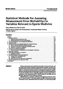
1 Introduction 1.1 Measurement error in exposure variables Measurement error in exposure variables is a known problem in many research areas. By definition, measurement error refers to the discrepancy between the true value and measured value of a variable (Thomas, Stram and Dwyer, 1993). In epidemiological research, measurement error can be due to recall bias when studies are conducted retrospectively requiring an individual to recall and report past events, or due to biological variations and instrument errors in laboratory experiments. Measurement error in exposures has been a long-term concern in relating exposures to health outcomes in epidemiological studies (Rothman, Greenland and Lash, 2008). In nutritional epidemiology, measurement error in dietary exposures has been a major impediment in relating long-term dietary intake to the occurrence of a disease (Ferrari et al., 2008). For example, the interest might be in the association between long-term intake of fruit and vegetable (hereafter, FV) and overall risk of cancer, as is the case in Boffetta et al. (2010). In such studies, dietary intake is usually assessed with a selfreport instrument, which is prone to measurement error. Measurement error in the selfreport instrument can be due to memory failure to recall past intakes over a long period of time (Agudo, 2004; Rosner and Gore, 2001). Therefore, it is impossible to measure long-term intake exactly. Using a dietary example, measurement error in dietary exposures can have two important effects in the parameter estimate that relates dietary intake to occurrence of a disease (Carroll et al., 2006). First, measurement error in dietary exposure can bias the parameter estimate that quantifies the association between dietary intake and occurrence of a disease (hereafter, diet-disease association). Second, there can be loss of statistical power to detect existing diet-disease associations. To illustrate these two important effects of measurement error, we use simulated data on the association between FV intake and reduction in the risk of cancer as an example (Figure 1.1).

1

Chapter 1

Random measurement error in FV intake leads to scatterplots (diamond dots) that are either higher or lower than true values (round dots). As a result, the regression slope that quantifies the association between FV intake and lower risk of cancer becomes more flattened (solid line) than the true slope (dashed line). This flattening effect quantifies the attenuation due to measurement error in the exposure. Attenuation refers to the bias of the association toward the null (Kipnis et al., 2003). Additionally, the variability around the regression line is much greater when the measured intake is used (diamond dots) than the variability around the regression line when the true intake is used (round dots), demonstrating loss of statistical power. The implication of the loss of power is that larger sample sizes are required to detect associations.

Figure 1.1: Simulated data showing the two important effects of measurement error on the association between reduction of risk of cancer (outcome) and FV intake (exposure): bias in the exposure-outcome association (attenuation) and loss of statistical power to detect associations. True intake (exposure) is shown by round dots and measured intake by diamond dots.

The focus of this thesis is on methods to adjust for the bias in the exposure-outcome associations, when exposure variables are measured with errors. When multiple

2

Introduction

exposures are measured with correlated errors, the exposure-outcome association can be biased in any direction (Day et al., 2004; Michels et al., 2004; Rosner et al., 2008). The exposure measurement error problem has prompted much methodological research, initially, on understanding the effects of measurement error on exposureoutcome associations and, more recently, on developing statistical methods to correct for exposure measurement error (Buonaccorsi, 2010; Carroll et al., 2006).

1.2 Measurement error in dietary exposure assessment The commonly used self-report instruments for measuring dietary intakes include food dietary questionnaires (DQs), 24-hour dietary recalls (24HRs) and dietary records (Agudo, 2004; Black, Welch and Bingham, 2000). In measuring dietary intake with a DQ, a wide range of food items are listed and individuals are asked to report their average frequency of consumption and average amount consumed over a long period of time, typically between several months to a year. A major drawback associated with the use of the DQ is memory failure to recall past intake. In the 24HR, however, subjects are asked to report their intake within 24 hours prior to the assessment time. Similar to the DQ, 24HR is also prone to recall bias, but to a lesser extent. Additionally, a single 24HR is unreliable in measuring long-term intake, unless administered multiple times per individual (Agudo, 2004). Unlike DQ and 24HR, in dietary records, an individual keeps a record of actual intake of foods consumed at the time of consumption for a specified period (Willet, 1998). Measuring food intake with the dietary record can lead to individuals changing their food intake patterns, when they realize that their intake is being monitored. This could lead to misreporting of true intake in the dietary record (Johnson, 2002). Further details on dietary assessment methods can be found in Al-Delaimy et al. (2005), Bingham et al. (1997), Bingham et al. (1994) and Block (1982, 1989).

1.3 Common measurement error terminologies, types and structures Measurement error can either be systematic or random. Systematic error arises when an individual consistently overestimates or underestimates his true level of exposure

3

Chapter 1

(Agudo, 2004). Random error, however, arises when an individual sometimes overestimates and sometimes underestimates true level of exposure. Exposure measurement error can either be nondifferential or differential. Nondifferential error occurs when the measured exposure contains no extra information about the health outcome other than what is contained in true exposure; error is said to be differential otherwise (Carroll et al., 2006, p. 36). In the FV intake-cancer example, if measurement error is nondifferential, measured FV intake in a single day should not contribute extra information about the risk of cancer other than what is contained in true long-term FV intake. On the other hand, if measurement error in reported FV intake depends upon whether an individual has cancer or not, especially due to recall bias when such a study is conducted retrospectively, then the measurement error will be differential (Thomas et al., 1993). To define different types of measurement error using the FV intake example, we denote self-report intake by 𝑄𝑄, unknown long-term true intake by 𝑇𝑇 and measurement error in self-reported intake by 𝜀𝜀𝑄𝑄 .

Measurement error structure can either be of classical or Berkson type. Classical error occurs when true intake is measured with error, such that the variability in the measured intake is greater than the variability in true intake. An example of classical measurement error structure is given by 𝑄𝑄 = 𝑇𝑇 + 𝜀𝜀𝑄𝑄 .

(1.1)

Berkson error, on the other hand, occurs when true intake is the sum of measured intake and measurement error, such that the variability in true intake is greater than the variability in the measured intake (Berkson, 1950). An example of Berkson error structure is given by 𝑇𝑇 = 𝑄𝑄 + 𝜀𝜀𝑄𝑄.

(1.2)

An example where Berkson error occurs is when individuals are classified into groups and all group members are assigned the same exposure value, say, the mean of true intake within that group; however, true intake for individuals within the same group 4

Introduction

would differ from the assigned intake values (Thomas et al., 1993). Exposures can also be measured with a mixture of Berkson and classical error as shown in Carroll et al. (2006, p. 51). The structure of measurement error can either be additive (as in expression (1.1)) or multiplicative. Multiplicative error arises when the magnitude of error increases with the quantity of true intake, such that larger true intake values are measured with larger error (Guolo and Brazzale, 2008). Multiplicative error is usually common with dietary intakes (Carroll et al., 2006). An example of a multiplicative measurement error structure can be given as 𝑄𝑄 = 𝑇𝑇𝜀𝜀𝑄𝑄 .

(1.3)

Exposure measurements can either be unbiased (e.g., as shown in expression (1.1)) or biased. Intake measurements are biased if the average value does not equal the true mean value, meaning that there is systematic error in Q. With multiple replicate self-report measurements (denoted by j for replicate and i for an individual), an example of additive measurement error structure with both systematic and random error components can be given by 𝑄𝑄𝑖𝑖𝑖𝑖 = 𝛽𝛽0 + 𝛽𝛽𝑄𝑄 𝑇𝑇𝑖𝑖 + 𝑟𝑟𝑄𝑄𝑖𝑖 + 𝜀𝜀𝑄𝑄𝑖𝑖𝑖𝑖 ,

(1.4)

where 𝛽𝛽0 quantifies overall constant bias and 𝛽𝛽𝑄𝑄 quantifies overall bias that is related

to the level of intake (Kipnis et al., 2001); 𝑟𝑟𝑄𝑄𝑖𝑖 is referred to as person-specific bias and

describes the fact that two individuals who consume the same amount of food will

systematically report their intakes differently (Carroll et al., 2006). For further details on measurement error structures, see Buonaccorsi (2010), Carroll et al. (2006) and Fuller (2006). In Figure 1.2, systematic and random measurement errors are juxtaposed; also shown are the components of an additive measurement error structure that is shown in expression (1.4).

5

Chapter 1

Figure 1.2 Schematic representation of common measurement error structures: systematic, random and both errors.

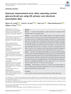
In Figure 1.3, the additive measurement error structures are presented graphically using an example of simulated intake data for an individual. In each graph, the solid horizontal lines represent an individual’s usual intake, defined as the average intake for the ten consumption days. When daily intake is measured with random error only, usual intake is measured accurately, i.e., with no bias as shown in Figure 1.3(a), but imprecisely leading to an inflated variance as shown by wider width of the green solid

6

Introduction

density curve in Figure 1.3(d). Figure 1.3(b) shows a situation where intake is measured with systematic error (here, constant bias only), and in this case intake is consistently overestimated with a distribution that is shifted to the right of the true distribution, but with the same variance as for the true intake (Figure 1.3(d), blue solid curve). In other cases, however, systematic error can lead to consistent underestimation of intake. Further, when intake is measured with both systematic and random errors, daily intake might be sometimes overestimated and sometimes underestimated, leading to an upward bias in the usual intake as shown in Figure 1.3(c) and an inflated variance as shown in Figure 1.3(d), red solid curve. In other cases, however, where intake is measured with both systematic and random errors, usual intake can be underestimated or overestimated. The wavy lines represent within-individual variation in daily intakes (Figure 1.3(a), (b) and (c)).

7

Chapter 1

Figure 1.3: A graphical representation of three common types of additive measurement error structures using simulated data when daily intake is measured with random error only, systematic error only and both systematic and random error. The horizontal lines represent usual intake; the black dots represent true intake values per consumption day; the dots in other colours represent measured intake values. Figure 1.3(d) compares an individual’s daily intake distributions for true intake and measured intakes.

1.4 Common methods to correct for measurement error in continuous exposures Five common bias-adjustment methods are described in this section. They are summarized in Table 1.1.

8

Introduction

1.4.1

Regression calibration

Regression calibration is the most commonly used method to adjust for the bias in the exposure-outcome associations caused by measurement errors in the exposure variables (Freedman et al., 2008; Guolo and Brazzale, 2008; Messer and Natarajan, 2008; Rosner, Spiegelman and Willett, 1990; Rosner, Willett and Spiegelman, 1989). This method is widely used because of its simplicity. The general idea of regression calibration is to estimate the conditional expectation of true exposure given the exposure measured with error and other covariates assumed to be measured without error. The estimated expected values are used in place of the unknown true exposure to estimate the association between the exposure and an outcome. Application of regression calibration requires additional information on the unobserved true exposure. This information is usually obtained from a validation study with unbiased measurements for true exposure (Kipnis et al., 1999; Kipnis et al., 2003). A validation study is often smaller than the main study and can be a random sample of subjects in the main study. To apply regression calibration, measurement error in the exposure is assumed to be nondifferential (Keogh and White, 2014). The method usually leads to consistent estimators of the association parameter (Guolo and Brazzale, 2008). 1.4.2

Likelihood method

The use of the likelihood method to correct for exposure measurement error requires specification of a parametric model for every component of the data, namely, the relation between the outcome of interest and the true exposure (hereafter, disease model), the relation between true exposure and covariates such as age and BMI (hereafter, exposure model) and the relation between measured exposure and the true exposure (hereafter, measurement error model). Subsequently, the likelihood function is obtained by integrating the product of the three densities over the latent true exposure variable (Guolo and Brazzale, 2008). The likelihood function is maximized to estimate the model parameters using either numerical methods or analytical approximations (Guolo and Brazzale, 2008). The method requires a validation study with multiple replicates of the unbiased measurements in order to specify the distribution of the true exposure. The likelihood method assumes nondifferential error

9

Chapter 1

(Thoresen and Laake, 2000). If correctly specified, the likelihood method can be more efficient than simpler measurement error correction methods such as regression calibration. This method, however, is rarely used in practice due to its computational burden and difficulty to specify parametric assumptions correctly. Moreover, it is often difficult to understand robustness of the likelihood method to model assumptions (Carroll et al., 2006). 1.4.3

Simulation Extrapolation (SIMEX)

SIMEX is a simulation-based method, sharing the simplicity and generality of regression calibration, but can be computationally prohibitive (Carroll et al., 2006). The method was proposed by Cook and Stefanski (1994) and has been developed further (Carroll et al., 1996; Lin and Carroll, 1999; Stefanski and Cook, 1995). The SIMEX method requires knowledge of the measurement error variance. Thus, a validation study with at least two replicates of the unbiased measurements is required. The following steps are followed to adjust for the bias in the association using the SIMEX method (Carroll et al., 2006). First, extra measurement error is added to the exposure measurements, creating a dataset with larger measurement error variance; this data generation step is repeated a large number of times. Second, the disease model is fitted and the association parameter estimated from each of the generated datasets in step one, then the average of the association parameter estimate is computed. Third, the above steps are repeated by adding various magnitudes of extra measurement error. Fourth, the average parameter estimates are plotted against the magnitude of added measurement error variance and then an extrapolant function is fitted. Lastly, the extrapolation is done to the ideal case of no measurement error to obtain the biascorrected estimate. The method assumes nondifferential error and is well suited for exposures measured with additive or multiplicative error (Guolo and Brazzale, 2008). 1.4.4

Bayesian methods

Bayesian methods have been used to adjust for measurement error in the covariates (Dellaportas and Stephens, 1995; Huang, Chen and Dagne, 2011). To adjust for the exposure measurement error with the Bayesian method, the following steps are followed (Carroll et al., 2006, p. 206-207). Similar to the likelihood method, a 10

Introduction

parametric model is specified for each component of the data and a likelihood function is formed. In the Bayesian framework, the parameters are assumed as random, unlike in the likelihood method where the parameters are assumed as fixed. Prior distributions are specified for the parameters in the model. Lastly, the posterior summary measures for the association parameter estimates are computed. The computation can be done with either a flexible sampling-based Markov chain Monte Carlo (MCMC) (Gelman and Hill, 2007) or a more computationally efficient non-sampling based integrated nested Laplace approximation (INLA) (Muff, 2015; Rue, Martino and Chopin, 2009). Despite the flexibility of Bayesian MCMC, it can be computationally intensive. Similar to the likelihood method, application of Bayesian method requires a validation study with multiple replicates of the unbiased measurements in order to specify the distribution of the true exposure. The method is suitable for nondifferential errors. 1.4.5

Multiple Imputation

Multiple imputation is a standard technique for handling data that are missing at random (Rubin, 1987). This method was proposed to adjust for measurement error in continuous exposures (Cole, Chu and Greenland, 2006; Freedman et al., 2008). To apply the multiple imputation method, the true exposure is assumed as missing data and is imputed multiple times by drawing from a distribution of the true exposure given all the observed data, including the outcome (Keogh and White, 2014). The multiple imputation method can accommodate differential error, because true exposure is imputed dependent on the outcome. The conditional distribution of the true exposure given the outcome and other observed data is often unknown. To estimate this conditional distribution, a validation study is required with data on (a) the study outcome and (b) multiple replicates of the unbiased measurements per individual. Using the estimated conditional distribution, the true exposure is imputed multiple times per individual to account for the uncertainty in the imputed exposure values. To each imputed dataset, the exposure-outcome model is fitted and the resulting association estimates are combined to obtain a pooled mean estimate (Rubin, 1987). The pooled mean estimate yields the bias-corrected estimator for the true exposureoutcome association (Messer and Natarajan, 2008).

11

Chapter 1

Table 1.1: Summary details for common measurement error adjustment methods Methods

Error assumption

Regression calibration

Nondifferential

Likelihood

Nondifferential

SIMEX

Nondifferential

Bayesian

Nondifferential

Multiple imputation

Differential

Required data • Validation study with unbiased exposure measurements

• Validation study with at least two replicates of unbiased exposure measurements per subject • Validation study with at least two replicates of the unbiased exposure measurements per subject

• Validation study with at least two replicates of the unbiased measurements per subject • Prior distributions for the model parameters • A validation study with (i) outcome data and (ii) at least two replicates of the unbiased exposure measurements per subject

12

Steps 1) Conditional expectation of true exposure given observed data is estimated 2) The expected values are used in place of unknown true exposure to estimate the exposureoutcome association 3) Standard error of the association parameter can be estimated using either bootstrap or asymptotic methods 1) Parametric model is specified for each component of the data, i.e., the outcome model, exposure model and measurement error model 2) The likelihood function is formed and maximized 1) Extra error is added to the measured exposure measurements to generate a new dataset 2) Association parameter is estimated from the generated dataset 3) The above steps are repeated many times and the mean estimate of the association parameter is computed 4) Steps1-3 are repeated for various magnitudes of extra-added error 5) The average association estimates are plotted against the magnitude of extra-added error and a trend is established 6) The trend is extrapolated back to the case of no error to obtain the SIMEX estimate 1) Model is specified for each data component and the likelihood function is formed 2) Prior distribution is specified for each model parameter 3) Posterior distribution is estimated and summary measures computed for the association parameter estimate 1) True exposure is imputed multiple times by drawing from a distribution of the true exposure given all the observed data, including the outcome 2) The exposure-outcome model is fitted to each imputed dataset to estimate the association 3) The association estimates are combined to obtain pooled mean estimate

Introduction

1.5 Current challenges Most validation studies in nutritional research stop at describing the correlation of measured intake with true intake. Studies that look at the quantitative effects of measurement error in dietary intakes on estimated associations between intake and health outcomes are rare. Additionally, the effects of dietary intakes on health outcomes are usually weak and are marred by inconsistencies. These inconsistencies are partly due to measurement error in intake, because many nutritional studies are based on questionnaires or interviews that contain a large amount of measurement error. Conducting a multiple-replicate validation study, besides the main study, however, is limited because it is costly. As a result, some epidemiological studies either conduct a single–replicate validation study or do not conduct a validation study at all. Among the commonly used measurement error correction methods (see Table 1.1) only regression calibration can be used for single-replicate calibration studies. However, regression calibration has not been applied and evaluated for a single-replicate validation study with zero-inflated measurements for the calibration response. For a study that does not include an internal validation study, the challenge in dealing with exposure measurement error is even bigger. The challenge is how to use external validation data from other similar studies to adjust for the bias in the exposure-outcome association. When exposures are measured with correlated errors, it can be very difficult to predict the direction and strength of the association (Marshall, Hastrup and Ross, 1999). The difficulty is due to contamination effect of the confounder measurement error (Freedman et al., 2011). Even though the problem due to contamination effect has been widely acknowledged in the literature, there is a lack of practical methods to quantify this effect in a specific epidemiologic study, both in terms of the approximate magnitude of the effect, and its direction. Measurement error problem is also common in physical activity research, where instruments, such as physical activity questionnaires, physical activity recalls and accelerometers, are used to monitor an individual’s long-term level of physical activity (Ferrari, Friedenreich

13

Chapter 1

and Matthews, 2007; Hills, Mokhtar and Byrne, 2014; Lim et al., 2015; Nusser et al., 2012; Tooze et al., 2013). Regarding the accelerometry research, various accelerometer models have currently been developed. However, some of these new accelerometer models have not been properly validated in field situations. Despite the widely recognized measurement error in the accelerometer, some accelerometers have been used to validate other instruments, such as physical activity questionnaires, in measuring physical activity (Lim et al., 2015). Therefore, if an instrument is validated against the accelerometer, and the accelerometer itself has considerable measurement error, the observed validity in the instrument being validated will misrepresent the true validity. These challenges constitute the motivation for the work in this thesis. The work in this thesis will address the following research questions emanating from the abovementioned challenges: (i) When only a single-replicate validation study with zero-inflated measurements is available, can the current methods be adapted to adjust for exposure measurement error? (ii) When there is no internal validation study, can a practical method be proposed that uses external validation data to adjust for the bias in the exposure-outcome associations? (iii) How large is the error in physical activity as measured by an accelerometer in free-living individuals and what is the impact of this error when accelerometer is used to validate other instruments?

1.6 Objectives of the study The research in this thesis aims to address the aforementioned research questions. The key objectives of this thesis are highlighted below: 1) To propose a two-part regression calibration to adjust for measurement error in dietary intakes not consumed daily, when only a single-replicate validation study is

14

Introduction

available. The task is to start with a simple linear calibration model and then improve it gradually. The improvement is done by modelling the excess zeros explicitly, handling heteroscedasticity in the response, exploring the optimal variable selection criteria, and identifying the optimal parametric forms of the continuous covariates in the calibration model, 2) To assess the performance of the proposed two-part regression calibration model in a simulation study with respect to: the percentage of excess zeroes in the response variable, the magnitude of correlation between probability of a non-zero response and the actual non-zero value, percentage of zeroes in the response and the magnitude of measurement error in the exposure, 3) To develop a multivariate method to adjust for the bias in the exposure-outcome association in the presence of mismeasured confounders when there is no internal validation study. The method combines external data on the validity of self-report instruments with the observed data to adjust for the bias in the exposure-outcome association, while simultaneously adjusting for confounding and measurement error in the confounders, 4) To validate a triaxial accelerometer in a recently concluded study by applying a measurement error model and quantifying the effects of measurement error in physical activity as measured by the accelerometer.

1.7 Thesis outline This thesis is organized into chapters. The contents of the remaining chapters are summarized below. In chapter 2, a two-part regression calibration model, initially developed for a multiple-replicate validation study design, is adapted to a case of a single-replicate validation study. The chapter further describes how to: handle the excess zeroes in the response, using two-part modelling approach; explore optimal parametric forms of the continuous covariates, using generalized additive modelling and empirical logit approaches, and how to select covariates into the calibration model. The adapted two-

15

Chapter 1

part model is compared with simple calibration models for episodically consumed food measured with error. A real epidemiologic case-study data is used. In chapter 3, a simulation study is conducted to assess the performance of the proposed two-part regression calibration by mimicking the case-study data in chapter 2. In chapter 4, a multivariate method is proposed to adjust for exposure measurement error, confounding and measurement error in the confounders when there is no internal validation study. The proposed method uses Bayesian Markov chain Monte Carlo method to combine prior information on the validity of self-reports with the observed data to adjust for the bias in the association. The method is compared with a method that ignores measurement error in the confounders. Further, a sensitivity analysis is performed to get insight into the measurement error structure, especially with respect to the magnitude of error correlation. The proposed method is illustrated with a real dataset. In chapter 5, a triaxial accelerometer is validated against doubly labelled water using a proposed measurement error model. Measurement error in the accelerometer is quantified with: (a) the bias in the mean level of physical activity, (b) the correlation coefficient between measured and true physical activity to quantify loss of statistical power in detecting associations, and (c) attenuation factor to quantify the bias in the associations between physical activity and health outcomes. In chapter 6, the main findings from the thesis are summarized and discussed in a general context. The study limitations are highlighted followed by suggestions for improvement and potential areas for future research. The chapter ends with concluding remarks.

16

Chapter 2

2 Use of two-part regression calibration model to correct for measurement error in episodically consumed foods in a single-replicate study design: EPIC Case Study 1 Abstract In epidemiologic studies, measurement error in dietary variables often attenuates association between dietary intake and disease occurrence. To adjust for the attenuation, regression calibration is commonly used. To apply regression calibration, unbiased (reference) measurements are required. Short-term reference measurements for foods not consumed daily contain excess zeroes that pose challenges in the calibration model. We adapted two-part regression calibration model, initially developed for multiple replicates of reference measurements per individual to a singlereplicate setting. We showed how to handle excess zero reference measurements by two-step modelling approach, how to explore heteroscedasticity in the consumed amount with variance-mean graph, how to explore nonlinearity with the generalized additive modelling (GAM) and the empirical logit approaches, and how to select covariates in the calibration model. The performance of two-part calibration model was compared with the one-part counterpart. We used vegetable intake and mortality data from European Prospective Investigation on Cancer and Nutrition (EPIC) study. In the EPIC, reference measurements were taken with 24-hour recalls. For each of the three vegetable subgroups assessed separately, correcting for error with an appropriately specified two-part calibration model resulted in about three fold increase in the strength of association with all-cause mortality, as measured by the log hazard ratio. Further found is that the standard way of including covariates in the calibration model can lead to over fitting. Moreover, the extent of adjusting for measurement error is influenced by forms of covariates in the calibration model. 1

Based on: Agogo, G. O., van der Voet, H., van ‘t Veer, P., et al. (2014). Use of Two-Part Regression Calibration Model to Correct for Measurement Error in Episodically Consumed Foods in a Single-Replicate Study Design: EPIC Case Study. PLoS ONE 9, e113160.

17

Chapter 2

2.1 Introduction Dietary variables are often measured with error in nutritional epidemiology. In such studies, long-term dietary intake (usual) dietary intake is assessed with instruments such as food frequency questionnaire and dietary questionnaire (Agudo, 2004; Kaaks et al., 2002; Willet, 1998). In these instruments, the queried period of intake ranges from several months to a year, resulting in difficulties to recall past intake of foods or food groups, the frequency of consumption, and the portion size. In general, the measurement error in dietary intake can either be systematic or random. Systematic error occurs when an individual systematically overestimates or underestimates dietary intake, whereas random error is due to random within-individual variation in reporting of dietary intake (Kaaks et al., 2002; Kipnis et al., 2003). The random error attenuates the association between dietary intake and disease occurrence, whereas systematic error can either attenuate or inflate the association. As a case study, we used the European Prospective Investigation on Cancer and Nutrition (EPIC) study. In EPIC, country-specific dietary questionnaires, hereafter DQ, were used to measure usual intake of various dietary variables or groups of dietary variables in different participating cohorts. With DQ measurements for usual intake, an association parameter estimate that relates usual intake to disease occurrence is often biased, typically towards the null (Fraser and Stram, 2001; Kaaks, 1997; Kipnis et al., 2003). Regression calibration is the commonly used method to adjust for the bias in the association between usual intake and disease occurrence, due to measurement error in the DQ. Regression calibration involves finding the best conditional expectation of true intake given DQ intake and other error-free variables (Freedman et al., 2008). The mean expected intake values are used in place of true usual intake in a disease model that relates dietary intake to disease occurrence. Regression calibration requires a calibration sub-study to obtain unbiased intake measurements to be used as the calibration response. Some prospective studies therefore include a calibration substudy that can either be internal or external. Internal calibration study consists of a

18

Use of two-part regression calibration

random sample of subjects from the main study, as was the case in the EPIC, whereas external calibration sub-study consists of subjects not in the main study but with similar characteristics as the main-study subjects (Slimani et al., 2002). In the calibration sub-study, unbiased (or reference) measurements are collected by shortterm instruments such as food records or 24-hour dietary recalls. In the EPIC study, regression calibration can also adjust for systematic error in the DQ due to the multicentre effect (Ferrari et al., 2008; Ferrari et al., 2004). In the EPIC calibration substudy, a 24-hour dietary recall (hereafter, 24-HDR) was used as the reference instrument. From each subject in the EPIC calibration sub-study, only a single measurement was obtained (Slimani et al., 2002). Dietary intake reported in the 24HDR for food not consumed daily is usually characterized by excess zeroes. These excess zeroes pose a challenge in the calibration model (Kipnis et al., 2009; Olsen and Schafer, 2001; Tooze et al., 2006; Zhang et al., 2011). With regression calibration, the excess zeroes can be handled using a two-step approach, where in the first step, consumption probability is modelled and in the second step the consumed amount on consumption days is modelled (Tooze et al., 2006). The currently published studies on two-part regression calibration method require calibration sub-studies with at least two replicates of reference measurement per subject (Kipnis et al., 2009; Tooze et al., 2006; Zhang et al., 2011). Given a singlereplicate design of the EPIC study with zero-inflated reference measurements, however, the calibration models in the literature cannot be applied directly. Moreover, there is limited research on the performance of the two-part calibration model in a single-replicate study design for episodically consumed foods. Further, there is inadequate research on the effect of the standard theory of variable selection on the performance of a two-part calibration model in a single-replicate study design. The standard theory of selecting covariates into the calibration model states that confounding variables in the disease model must be included in the calibration model together with the covariates that only predict dietary intake (used as the response in the calibration model) but not the risk of the disease (Carroll et al., 2006; Kipnis et al., 2009).

19

Chapter 2

To fill the aforementioned gaps, we developed a two-part regression calibration model to adjust for the bias in the diet-disease association caused by measurement error in episodically consumed foods, in the presence of a single-replicate calibration substudy. The second goal was to assess the effect of reducing the number of variables selected into the two-part calibration model based on the standard theory. As a working example using the EPIC study, we studied the association between intakes of each of the three vegetable subgroups: leafy vegetables, fruiting vegetables, and root vegetables with all-cause mortality. We described how to handle the excess zeroes, skewness and heteroscedasticity in the reference measurements used as the response in the calibration model, nonlinearity, and how to select covariates into the calibration model. We showed that a suitably specified two-part calibration model adjusts for the bias in the diet-disease association caused by measurement error in self-reported intake. We further showed that the extent of adjusting for the bias is influenced by how the calibration model is specified, mainly with respect to forms of the continuous covariates.

2.2 Materials and Methods 2.2.1

Study subjects

EPIC is an on-going multicentre prospective cohort study to investigate the relation between diet and the risk of cancer and other chronic diseases. The study consisted of 519,978 eligible men and women aged between 35 and 70 years and recruited in 23 centres in 10 Western European countries (Riboli et al., 2002; Slimani et al., 2002). The 10 participating countries were: France, Italy, Spain, United Kingdom, Germany, The Netherlands, Greece, Sweden, Denmark, and Norway. The study populations comprised of heterogeneous groups. In most centres, study populations were based on general population while some consisted of participants in breast screening programs (Utrecht, The Netherlands; and Florence, Italy), teachers and school workers (France) or blood donors (certain Italian and Spanish centres). In Oxford, most of the cohort was recruited among subjects with interest in health or on vegetarian eating. Only women were recruited in France, Norway, Utrecht (The Netherlands) and Naples (Riboli et al.,

20


2002). Information on usual dietary intake, lifestyle, environmental factors and anthropometry was collected from each individual at baseline. The dietary intake information was assessed with different dietary history questionnaires, food frequency questionnaires or a modified dietary history developed and validated separately in each participating country (Riboli et al., 2002). The questions asked in the questionnaires included the frequency of consumption over the past 12 months preceding the administration, categorized into the number of times per day, per week, per month or per year. A calibration sub-study was carried out within the entire EPIC cohort by taking a stratified random sample of 36,900 subjects. In the calibration sub-study, a 24HDR was administered once per subject using a specifically developed software program (EPIC-SOFT) designed to harmonize the dietary measurements across study populations (Slimani, Valsta and Grp, 2002). We used EPIC dietary intake data for leafy vegetables, fruiting vegetables and root vegetable sub-groups as a working example. We further assumed measurements from the 24-HDR (in g/day) as the reference measurements and the intake reported in the DQ as the main-study measurements. We excluded subjects with missing questionnaire data, missing dates of diagnosis or follow up, in the top and bottom 1% of the distribution of the ratio of reported total energy intake to energy requirement. We further excluded subjects with a history of cancer, myocardial infarction, stroke, angina, diabetes or a combination of these diseases at baseline. As a result, data for 430,215 subjects were eligible for the analyses. In the analysis, the data from the following centres were excluded: Umeå and Norway for leafy vegetables and Norway for fruiting vegetables. The decision to exclude these data was based on the inclusion criteria as stipulated in the EPIC analysis protocol. 2.2.2

Regression calibration model

In epidemiological studies, the interest is mainly in the association between an exposure and the risk of disease. In our working example, we were interested in the association between intake of vegetable subgroups and all-cause mortality. If the true

21

Chapter 2

usual intake of a vegetable subgroup is known, then the true association can be modelled by a generalized linear model (GLM) as

ϕ{E(Y | T , Z= )} βT T + β ZT Z ,

(2.1)

where Y is a disease outcome, here, an indicator for mortality, T is true usual dietary intake of a vegetable subgroup, Z is a vector of error-free confounding variables and φ is a function linking the conditional mean and the linear predictor. The coefficient

βT

quantifies the association of interest and β ZT is a vector of coefficients for the confounding variables. If dietary intake is measured with error, then

βT would mostly

be underestimated. Regression calibration is the most commonly used method to adjust for the bias in estimating

βT caused by measurement error in the DQ. To describe regression

calibration, we denote reference measurement from the 24-HDR by R, main-study measurement from the DQ by Q, and the covariates that only predict vegetable intake and not all-cause mortality by C. Therefore, a set of all covariates that possibly relate to usual intake is given by 𝐗𝐗 = {𝐙𝐙, 𝐂𝐂}. Regression calibration involves finding the best prediction of conditional expectation of true intake given DQ intake and other

covariates assumed to be measured without error (Kipnis et al., 2009). The conditional expectation from regression calibration is denoted by E(T | Q, X) . A major challenge in fitting the calibration model is that true usual intake is unobservable and cannot be measured exactly. As a result, a reference measurement is used in place of the latent true intake in the calibration model. Measurement from a valid reference instrument should be unbiased for true intake, and should have random errors that are uncorrelated with the measurement errors in the DQ (Kipnis et al., 2003). We, therefore, made two strong assumptions: that the 24-HDR is unbiased for true usual intake and measurement error in the 24-HDR is uncorrelated with the measurement error in the DQ. We denote the calibration model by:

E(T | Q, X) = E( R | Q, X)

22

(2.2)


We assumed in model (2.2) that measurement error in Q does not provide extra information about Y other than that provided by T. The measurement error in Q is, therefore, said to be non-differential. In model (2.2), R is modelled as a function of Q and X using standard regression methods, where a suitable distribution for the error terms and a suitable parametric form of each covariate in X is chosen. In this work, we considered only the case of a single dietary intake variable measured with error. In our data, the correlation between the vegetable subgroups and the confounders, as measured by the questionnaire, were low justifying their omission, as the contamination effect of the measurement error in these variables on the correction factor for our dietary intake of interest would be negligible. 2.2.2.1

Excess

zeroes,

heteroscedasticity

and

skewness

in

reference

measurements Vegetable subgroups considered in this study are not consumed daily. This results in many zero reference measurements reported on the 24-HDR. As a result, the reference measurements have a mixture of zeroes for non-consumers and positive intake for consumers. To handle these excess zeroes, we used a two-part approach to build a regression calibration model. In the first part, the probability of reporting consumption in the 24-HDR is modelled. In the second part, the consumed amount given consumption in the 24-HDR is modelled (Tooze et al., 2006). The first part involves discrete data and can be modelled either with logistic or probit regression, where the probability of consumption is modelled conditional on a given set of covariates. In the second part, the consumed amount given consumption can be modelled conditional on the covariates and by assuming a plausible family of densities (McCullagh and Nelder, 1989). The GLM model for the consumption probability (Part I) is parameterized as

P( R > 0 | Q, X)= φ −1 (α q Q + α XT X)= π Q , X , where

φ −1 can be either inverse-logit or inverse-probit function. Similarly, the GLM

model for the consumed amount (Part II) is parameterized as

23

Chapter 2

T X) µQ , X , E( R | Q, X; R >= 0) g -1 ( β q Q + β X=

where g

−1

can be an inverse of any plausible link function. Thus, the calibration

model (2.2), adapted to two-part form to handle the excess zeroes in the reference measurements used as the calibration response is parameterized as

E( R | Q, X= ) φ −1 (α q Q + α XT X) × g −1 ( β q Q + β XT X= ) π Q , X µQ , X . The true usual intake can thus be predicted from this two-part calibration model. We denote the prediction from this two-part calibration model by

ˆ R | Q, X) = πˆ µˆ . E( Q,X Q,X

(2.3)

Another challenge is how to handle distribution for the consumed amount that is commonly

right-skewed

and

with

heteroscedastic

variance.

To

handle

heteroscedasticity, we applied a GLM approach, where the variance is linked to the mean as

σ 2 ( R | Q, X; R > 0) = ψ {Ε( R | Q, X; R > 0)} , where ψ is a function that links the conditional variance with the conditional mean of consumed amount, σ 2 (·|·) denotes the conditional variance, and E(·|·) denotes the conditional expectation (Manning, Basu and Mullahy, 2005). The advantage of using the GLM approach is that the consumed amount can be predicted directly without transforming the response values in Part II of the calibration model. To determine the optimal relation between the conditional variance and the conditional mean, the GLM model shown above is parameterized using a class of power-proportional variance functions as follows

, X; R > 0) κ {E( R | Q, X; R > 0)}λ , σ 2 ( R | Q= where κ denotes the coefficient of variation, λ is a finite non-negative constant. This power variance function can be rewritten in a linear logarithmic form as

σ ( R | Q, X; R > 0) =a + b log{E( R | Q, X; R > 0)} ,

(2.4)

where a = (log κ ) / 2 and b = λ / 2 . In model (2.4), a value of λ equals zero refers to a classical nonlinear regression with constant error variance, λ equals one refers to a

24


Poisson regression with the variance that is proportional to the mean, where 𝜅𝜅 > 1

indicates degree of over dispersion. Similarly, λ equals two with 𝜅𝜅 > 0 refers to a

gamma model with the standard deviation that is proportional to the mean (Manning

and Mullahy, 2001). To explore a suitable value for λ to identify the right GLM model, we plotted centre-specific log-transformed standard deviation versus centre-specific

log-transformed mean, separately for each of the three vegetable subgroups reported in 24-HDR in the EPIC study. The value of λ is estimated as twice the slope of the fitted regression line (see model (2.4)). The GLM model considered here can accommodate family of densities with skewed (asymmetric) distributions. We chose to use graphical method to identify λ due to its simplicity as opposed to estimation methods such as the maximum likelihood (MLE). 2.2.2.2

Nonlinearity and variable transformation

The relation between dietary intake variables is often nonlinear. To explore the form of relation between consumption probability as reported on 24-HDR and usual intake as reported on DQ, we applied two techniques: the empirical logit plot, and the nonparametric generalized additive model (GAM). With the empirical logit technique, we categorized DQ intake, starting with the category of never-consumers followed by 10 g/ day intake intervals. In each category, we computed the logit of consumption as reported on the 24-HDR. The formula for the empirical logit transformation used is given by (Cox, 1970; McCullagh and Nelder, 1989)

 yi + 0.5  log  ,  ni − yi + 0.5 

(2.5)

where yi is the number of individuals who reported consumption on the 24-HDR and

ni is the number of individuals in the ith DQ-category. The addition of 0.5 to both the numerator and the denominator of the logit function serves to avoid indefinite empirical logit values when yi = ni or yi = 0 , and this particular value minimizes the bias in estimating the log odds (McCullagh and Nelder, 1989). The estimated empirical logit (computed from the 24-HDR intake) is plotted against the mean intake in the

25

Chapter 2

respective DQ-category (computed from the DQ intake). We fitted a loess curve to the resulting scatterplots to have a visual inspection of the form of relation between the two variables (Weiss, 2006). We further made the empirical logit plots for each of the participating country in the EPIC study. With the GAM technique, we obtained an optimal smoothing splines for the relation between the consumption probability reported in 24-HDR and DQ intake based on generalized cross validation criterion (GCV) (Hastie and Tibshirani, 1999). We fitted the GAM model for consumption probability, assuming a binomial distribution and a logit link function using the mcgv package in R (Wood, 2012). In the GAM model, we included confounding variables in the disease model (Z). We used the partial prediction plot from the smoothed DQ component to identify plausible forms of parametric transformations for the DQ (Cai, 2008). From the selected set of parametric transformations, Akaike Information Criterion (AIC) was used to identify the optimal parametric transformation. Similar to the consumption probability part, we used the GAM approach to explore the optimal form of the DQ intake in the consumed amount part of the calibration model. 2.2.2.3

Variables inclusion in the calibration model

The theory of regression calibration states that all confounding variables in the disease model must also be included in the calibration model in addition to the covariates that only predict the response in the calibration model (Kipnis et al., 2009). We used the same set of confounding variables in Agudo (2004) that studied the relation between intake of vegetables and mortality in the Spanish cohort of EPIC. The eight confounding variables were: BMI (kg/m2), smoking status (never, former, current smoker), physical activity index (inactive, moderately inactive, moderately active, active), lifetime alcohol consumption (g/day), level of education (none, primary, technical, secondary, university), age at recruitment (years), total energy (kcal), and sex (male/female). The covariates that only predict intake as measured 24-HDR were selected based on their statistical significance in the calibration model (2.3). We

26


included plausible two-way interaction terms of DQ intake variable with the other covariates in the calibration model. We hereafter refer to each of the calibration model with covariates selected using the standard theory with the prefix “standard”, here, standard two-part calibration model. The covariates are included twice in the two-part calibration model (i.e., in each part of the two-part model), thus posing a threat to over fitting. Moreover, some disease confounding variables might not necessarily predict true usual intake. We therefore conducted a backward elimination on the standard twopart calibration model based on a significance level α of 0.2. We chose 0.2 to ensure that no significant covariates are excluded from the model. We hereafter refer to each of the reduced version of the standard calibration model with the prefix “reduced”, here, reduced two-part calibration model. To assess the power of the probability part of the two-part calibration model to correctly discriminate consumers from non-consumers as reported in the 24-HDR, we used the Area under the curve from the Receiver operating characteristic curve of the fitted logistic model (Steyerberg, 2009). For the consumed amount part, we assessed the predictive power of the model based on the root mean squared error and the mean bias (Hastie, Tibshirani and Friedman, 2009). In building the two-part calibration model, we conducted country-specific rather than centre-specific regression calibration models to obtain stable estimates given the relatively smaller sample sizes in each centre (Ferrari et al., 2008). We also fitted other forms of regression calibration models to compare with the developed two-part calibration model. These forms of the other calibration model include (i) A two-part calibration model similar to the developed one but with untransformed DQ. We hereafter refer to this model as “Two-part (untransformed DQ)”. The aim of fitting this model was to assess the effect of nonlinearity on the performance of a two-part calibration model. (ii) A one-part calibration model with untransformed DQ and with the usual assumptions of a classical linear model. This is the calibration model commonly used by epidemiologists to adjust for the bias in the diet-disease

27

Chapter 2

association. In this model, two strong assumptions are made, namely, normality and linearity. The aim of fitting this calibration model was to quantify the inadequacy in adjusting for the bias in the diet-disease association when these assumptions are violated. In each of these two forms of calibration models, we used the same set of covariates as in each part of the standard two-part calibration but with different parametric forms of the DQ intake as explained above. We conducted a backward elimination (α = 0.2) on each of these forms of regression calibration models to obtain their reduced forms. Subsequently, we used a Cox proportional hazard model in model (2.1) to study the association between usual intake of vegetable subgroups and all-cause mortality (Cox, 1972). The Cox proportional hazards model was stratified by centre and sex. To explore the form of relation between usual intake of each of the three vegetable subgroups and all-cause mortality in the Cox model, we plotted the log hazard ratio estimate against median intake in each DQ category (Sainani, 2009). We used bootstrap procedure to compute correct standard error for the log hazard ratio estimate. The bootstrap approach accounts for the uncertainty in the calibration process. We used centre-stratified bootstrapping on the calibration sub-study. To each bootstrap sample, the main-study data was added and regression calibration model fitted to generate replicate versions of E( R | Q, X) for each subject in the entire EPIC cohort (Cassell, 2007). To each replicate data, the Cox model was fitted yielding an estimate of log hazard ratio with a standard error. The within-calibration and betweencalibration variances were combined using Rubin’s formula to account for the uncertainty in the calibration process (Boshuizen et al., 2007; Geert Molenberghs, 2007; Rubin, 2004). The Rubin’s formula used to estimate the standard error for the log hazard ratio estimate is

(

)

(

)

2

m 2 1 m ˆ ) + 1 + 1  1  ˆ SE( = σ Τ (β ) β ∑ i    ∑ βi − β , m i 1=  m  m − 1  i 1 = 2

28

(2.6)


where

σ 2Τ ( β ) is the total variance of the mean of log hazard ratio estimate from m

calibrated

SE( βˆi )

samples,

(

)

is

the within-calibration

standard

error,

and

2

 1  m ˆ   ∑ βi − β is the between-calibration variance.  m − 1  i =1 We fitted a Cox proportional hazards model that ignores the measurement error in the DQ intake. This method is hereafter referred to as the naïve method. In the naïve method, the DQ intake measurements were used to study the association between usual intake of a vegetable subgroup and all-cause mortality.

2.3 Results In Table 2.1, a high percentage of zeroes is shown in the 24-HDR intake for each of the three vegetable subgroups, especially for root vegetable subgroup in most of the participating countries. The rather high percentage of zeroes in the 24-HDR suggests that these subgroups of vegetables are not consumed daily by everyone. The Pearson correlation coefficient for each of the three vegetable subgroups in each of the participating countries, as measured with 24-HDR and DQ, were rather low but mostly statistically significant. The boxplots for the distribution of the consumed amount on consumption events as reported in the 24-HDR showed positive skewed distributions for these dietary intake variables (Figure 2.1). These exploratory findings suggested a need to properly handle the excess zeroes, to choose either a suitable distribution or a correct transformation for the consumed amount reported in the 24-HDR in building a calibration model.

29

Chapter 2

Table 2.1: Country-specific summary measures for the percentage of zero intake measurements reported on 24-HDR (% R=0, non-consumers) and Pearson Correlation (ρ) for intake as measured by 24-HDR and DQ for leafy vegetables, fruiting vegetables and root vegetables. EPIC Study, 1999-2000

Leafy vegetables

Participating Countries

Fruiting vegetables

Root vegetables

N

% R=0

ρ

% R=0

ρ

% R=0

ρ

France

4735

42.8

0.17

44.4

0.10

71.6

0.06

Italy

3961

59.3

0.16

37.6

0.15

79.6

0.11

Spain

3220

48.9

0.34

31.7

0.22

76.1

0.12

UK

1313

68.2

0.16

40.8

0.19

59.3

0.23

Netherlands

4545

70.5

0.10

48.7

0.21

82.0

0.14

Greece

2930

67.9

0.10

29.5

0.13

83.2

0.03ns

4418

75.9

0.15

41.6

0.17

79.2

0.22

6132

70.5

0.19

34.9

0.24

67.2

0.17

Denmark

3918

77.4

0.09

41

0.21

61.8

0.40

Norway

b

58.5

0.12

Germany Sweden

a

1798

a

N is 3132 instead of 6132 for leafy vegetables in Sweden because data from Umeå were excluded from analysis based of the inclusion criteria in EPIC; b N refers to data for root vegetables only because data for Norway were excluded for leafy vegetable and fruit vegetable subgroups; ns means correlation is not statistically significant at α = 0.05, other correlation coefficients are highly significant with P < 0.0001.

30


Figure 2.1: The country-specific boxplots show the distribution of the consumed amount for those who reported consumption on the 24-HDR for leafy vegetables (LV), fruiting vegetables (FV) and root vegetable (RV) subgroups in the EPIC study, 1992-2000.

For each of the three vegetable subgroups, a linear trend is shown between the log of standard deviation and the log of the mean for the consumed amount reported in the 24-HDR (Figure 2.2). The linear trend is a clear evidence of a variance that increases with a mean (presence of heteroscedasticity). The slope (standard error) of least squares regression line fitted to the resulting scatterplots was estimated as 1.057 (0.085). For fruiting vegetables, the estimates were 0.994 (0.076). Likewise for root vegetables, the estimates were 1.021 (0.130). These slopes of the fitted lines were all close to the theoretical value of 1 for a GLM gamma model. Based on these exploratory findings, we chose a gamma GLM model for the consumed amount in part II of the two-part calibration model for each of the three vegetable subgroups. The correlation between each of the three vegetable subgroups ranged from 0.06 to 0.12 with total energy and from -0.07 to 0.05 with alcohol, as measured with the DQ. 31

Chapter 2

These low correlations suggest minimal contamination effect of measurement error on diet-disease association, hence justifying our choice not to adjust for measurement error also for these confounding variables.

Figure 2.2: Variance-mean relation for leafy vegetable intake (LV), fruiting vegetable intake (FV) and root vegetable intake (RV). The graph shows a least squares regression line fitted to the scatterplots of the logarithm of centre-specific standard deviation versus logarithm of centre-specific mean of the consumed amount for those who reported consumption on the 24HDR in the EPIC Study, 1992-2000. The approximately linear regression line suggests a variance that increases with the mean.

To explore the form of the DQ intake variable for the consumption probability part of the two-part calibration model, the loess curve fitted to the scatterplots of the empirical logit versus the mean intake in each DQ category showed a nonlinear relation between the logit of consumption as reported in the 24-HDR and the DQ intake (dotted lines in Figure 2.3). The GAM partial prediction plots showed similar behaviour. From the plausible set of parametric transformations for the DQ, here, square-root and logarithmic, we chose log-transformed DQ based on the AIC criterion for each model fitted to country-specific data. As a result, we fitted a logistic model with log-

32


transformed DQ and computed mean of the predicted logit of consumption in each category of the DQ. The loess curve fitted to the scatterplots of the mean predicted logit against the mean intake in a given DQ category is shown in the same figure (continuous line). The similarity of the two loess curves suggested the aptness of logtransforming DQ intake in the consumption probability model of leafy vegetables (Part I). The graphs for fruiting vegetables and root vegetables yielded similar results.

Figure 2.3: Country-specific empirical logit graphs for leafy vegetable intakes. The graph shows loess curves fitted to 1) the scatterplots for the empirical logit (dotted line) and 2) the mean of the predicted logit from a logistic model with log-transformed DQ (thick line) against the DQ category-specific means for leafy vegetable intake in the EPIC Study, 19922000. The similarity in the two logit curves suggests that a log- transformed DQ is appropriate for the consumption probability part of the two-part calibration model.

To explore the form of the DQ intake in the model for consumed amount (Part II), we fitted a GAM model with gamma distributed error terms and a log link function (as 33

Chapter 2

suggested by exploratory results). Based on partial prediction plots for the smoothed DQ intake component and using the AIC criterion, we chose a square-root transformed DQ intake for both leafy vegetables and root vegetables subgroups, and a logtransformed DQ intake for fruiting vegetables. In addition to the confounding variables in the Cox proportional hazards model (shown in section (2.2.2.3)), season of DQ administration, centre where the DQ was administered and the body weight of the participant were also included in the calibration model, because they predicted intake of each of the three vegetable subgroups. Other covariates included in the standard two-part calibration model were the transformed DQ intake and its two-way with sex, age, season, BMI and centre. We used the same set of covariates on each part of the standard two-part calibration model, but with additional quadratic term for age at recruitment in the consumed amount part of the model. In Table 2.2, we showed the remaining significant terms after a backward elimination on each part of the standard two-part calibration model separately for each of the three vegetable subgroups.

34


Table 2.2: Significant covariates (marked ×) in the reduced two-part calibration models, after a backward elimination on each part of the standard two-part regression calibration model with transformed DQ and with other covariates selected using the standard way of variable inclusion. EPIC Study, 1992-2000

Covariates

Main effects Qt BMI Smoking status Physical activity Lifetime alcohol Education Age Age2 Total energy intake Weight Center Season Sex Interaction terms Qt * sex Qt * age Qt * season Qt * BMI Qt * center

Leafy vegetables Part I Part II ×

Fruiting vegetables Part I Part II

× ×

× × × × × × ×

× × × × ×

× ×

×

× ×

× × ×

×

× ×

× × ×

× × × ×

× × ×

× × × ×

× ×

× × × ×

× × × ×

× ×

× × ×

× × ×

× × ×

×

Root vegetable Part I Part II

×

×

× ×

× × × ×

×

Qt is a transformed DQ; Part I, refers to consumption probability part of the two-part calibration model; Part II, refers to consumed amount part of the two-part calibration model; *, refers to an interaction term.

The areas under the curve from the ROC curve for the consumption probability part of the standard two-part calibration model and its reduced form were quite similar for each of the vegetable subgroups (Table 2.3). This suggest that some confounding 35

Chapter 2

variables and other two-way interaction terms of DQ intake with other covariates in the standard model do not necessarily predict the consumption probability and therefore should not be included in the calibration model. A similar remark could be made for the consumed amount part of the model, based on the root mean squared error and the mean bias, which were quite similar. Table 2.3: The area under the curve (AUC) from ROC curve for consumption probability (Part I), and root mean square error (RMSE) and mean bias for the consumed amount (Part II) of the standard and the reduced forms of two-part regression calibration models with transformed DQ

Vegetable

Part I

Mean Biasb

Subgroups

Models

AUC

RMSE

Leafy

Standard

0.6846

66.841

0.0223

Reduced

0.6843

64.578

0.0019

Standard

0.6305

118.823

0.0446

Reduced

0.6304

110.415

-0.0334

Standard

0.6413

68.626

0.0895

Reduced

0.6408

66.524

0.0883

Fruiting Root

a

Part II a

(

1 n ˆ = RMSE ∑ Ri − Ri n i =1

)

2

; b mean_bias =

(

1 n ˆ ∑ Ri − Ri n i =1

)

Figure 2.4, we fitted the smoothed curve to the scatterplots of the log hazard ratio estimate of dietary intake on all-cause mortality versus the median DQ intake in each DQ category. The graphical exploration showed approximately linear relations of DQ intake to all-cause mortality for each of the three vegetable subgroups. We therefore assumed a linear term for the DQ intake in the three fitted Cox proportional hazards models.

36


Figure 2.4: Assessment of linearity assumption of the DQ intake in the Cox proportional hazards model for leafy (LV), fruity (FV) and rooting (RV) vegetable subgroups. In each graph, a smoothed curve is fitted to the scatterplots of log hazard ratio estimate of vegetable subgroup intake on all-cause mortality versus DQ category-specific median intake (in grams). The approximately linear downward trend in each graph suggests an approximate linear relation and a beneficial effect of vegetable intake on the risk of all-cause mortality.

As expected, the log hazard ratio estimate for usual intake in the Cox model adjusted for measurement error in DQ intake were larger in absolute value than the naive estimate that ignores the measurement error. Similar remark was made for all the fitted forms of regression calibration models but the standard two-part calibration model with untransformed D (Table 2.4). The log hazard ratio estimates adjusted for the bias with the standard calibration models were smaller than those adjusted with the reduced calibration models, e.g., -0.265 for the standard two-part (transformed DQ) and -0.479 for the reduced two-part (transformed DQ) calibration model per 100g intake of root vegetables. The seemingly poor performance of the standard calibration models might be due to over fitting by covariates that did not significantly predict usual intake. The log hazard ratio estimate for root vegetables adjusted with the standard two-part calibration (with untransformed DQ intake) model (𝛽𝛽̂𝑇𝑇 = -0.107) was even smaller than 37

Chapter 2

the naïve estimate (𝛽𝛽̂𝑇𝑇 = -0.160). This suggests that a poorly specified functional form

of a continuous covariate in a calibration model can result in adjusted association

estimates that are more biased than the unadjusted estimates. The standard error of the log hazard ratio estimate, which is corrected for the uncertainty in the calibration, was larger than the uncorrected standard error for each of the calibration models. The underestimation of standard error was more severe for the standard calibration models. Further, the log hazard ratio estimate, which is calibrated with the reduced one-part linear calibration model, was smaller than that obtained with the reduced two-part (transformed DQ) model. Further, the predicted intake values for some subjects not in the calibration sub-study, in some cases were rather unrealistic. The unrealistic predictions were mainly from the standard calibration model with the untransformed DQ intake. The calibration models with the untransformed DQ intake resulted in a much smaller log hazard ratio estimate than their counterparts with the transformed DQ intake. This might be driven by extreme prediction from highly skewed DQ intake measurements in the calibration model. The effect of the extreme DQ values was further compounded by two factors: including the same covariate twice in the two-part calibration model and by the exponentiation effect due to the log link function used Part II of the calibration model. As a result, we assessed the sensitivity of the log hazard ratio estimate to these unreasonably high predicted values. Including these extreme predicted intake values resulted in massive change in the log hazard ratio estimate, mainly for the standard two-part calibration model with the untransformed DQ intake. For leafy vegetables, for instance, including the unrealistic predictions from the standard two-part calibration model with the untransformed DQ intake changed the estimate of log hazard ratio from -0.174 to -0.00518 per 100g intake. In Table 2.5 in the appendix, we present the percentages of these unrealistic predicted intake values, defined as extreme if it exceeded fivefold the ninety ninth percentile of the predicted usual intake. In the final analysis, we excluded these unrealistic values.

38

39

Root

1.36 2.49 3.06

1.11 1.14 2.92

1.24 1.99 3.24

SE ratioc

-0.160(0.026) -0.305(0.054;0.077) -0.107(0.060;0.167) -0.265(0.056;0.181)

-0.094(0.014) -0.123(0.031;0.034) -0.109(0.030;0.073) -0.228(0.035;0.131)

-0.144(0.027) -0.409(0.083;0.127) -0.174(0.089;0.278) -0.461(0.047;0.160)

𝛽𝛽̂𝑇𝑇 (SEa; SEb)

1.43 2.78 3.23

1.11 2.42 3.74

1.53 3.11 3.41

Standard model SE ratioc

standard error (×10-2) that accounts for the uncertainty in the calibration; SE ratioc is the ratio of SEb to SEa

SEa is the standard error (×10-2) for 𝛽𝛽̂𝑇𝑇 that does not account for the uncertainty in the calibration; SEb is the

-0.160(0.026) -0.342(0.060;0.082) -0.203(0.088;0.219) -0.479(0.070;0.214)

Naïve method One-part linear calibration Two-part(untransformed DQ) Two-part (transformed DQ)

Fruiting

Leafy

-0.144(0.027) -0.480(0.090;0.112) -0.395(0.092;0.183) -0.509(0.090;0.292) -0.094(0.014) -0.125(0.031;0.034) -0.161(0.030;0.034) -0.255(0.037;0.108)

Naïve method One-part linear calibration Two-part (untransformed DQ) Two-part (transformed DQ)

𝛽𝛽̂𝑇𝑇 (SEa; SEb)

Naïve method One-part linear calibration Two-part(untransformed DQ) Two-part (transformed DQ)

Methods

Vegetable subgroups

Reduced model

Table 2.4: Log hazard ratio estimate (standard error) per 100g usual intake of each of the three vegetable subgroups, calibrated with each of the three forms of regression calibration models in their reduced and standard forms


Chapter 2

2.4 Discussion In this work, we adapted a two-part regression calibration model initially developed for multiples of 24-HDR intake per individual for episodically consumed foods to a single replicate setting. We focused on dietary intakes with reference measurements that are skewed, heteroscedastic, and with substantial percentage of zeroes as reported on the 24-HDR. We further described how to explore and identify a suitable GLM model and a correct parametric form of a continuous covariate in the calibration model. As a result, we applied flexible GLM models that could simultaneously handle skewness and heteroscedasticity in the consumed amount. Thus, we avoided complications resulting from response transformation. We chose the log link function to stabilize the variance and to ensure positive prediction for usual intake (Raymond, 2010). The standard way of including variables in the calibration model states that all confounding variables in the disease model and those that only predict dietary intake but not the disease occurrence must be included in the calibration model. Given the complexity of the two-part calibration model, some confounding variables in the disease model do not necessarily predict dietary intake. This could pose a threat to over fitting the calibration model. We conducted a backward elimination on each part of the two-part calibration model separately. The reduced calibration model with only significant covariates seemingly outperformed its standard counterpart in adjusting for the association bias. Leaving out confounding variables from the calibration model is against the standard theory of regression calibration. Nevertheless, we argue that if the omitted covariates have no effect in the calibration model, they should be excluded and the calibration method should still be correct. We further found that assuming linearity in the calibration model when it does not hold in a calibration model can pose a serious threat to the model performance. Similarly, Thoresen (2006) found in a simulation study that a less specified calibration model can have a considerable impact on the degree of bias-adjustment. We observed that predicted values for some subjects not in the calibration sub-study were extremely large. The extreme predictions resulted mainly from standard calibration models with linear term for the DQ intake. In such a case, predictions are made outside the variable space on which the model is fitted. As a

40


consequence, the prediction space would extend more outside the variable space in the complex models. The consumption probability and the consumed amount for episodically consumed foods may be correlated. In each of the fitted two-part calibration models, we accounted for this correlation partly by allowing covariates to overlap on both parts of the two-part calibration model (Kipnis et al., 2009). With only a single 24-HDR intake measurement per subject, part of correlation not explained by the covariates cannot be estimated. In future studies, a sensitivity analysis can be performed to assess the effect of the part of the correlation that is not explained by the covariates. This can be done by varying the magnitude of the assumed positive correlation between the consumption probability and the consumed amount in a simulation study (see chapter 3). A limitation of this study is that we made some strong assumptions. First, we assumed the 24-HDR to be unbiased for true usual intake. Second, we assumed that the errors in the 24-HDR are uncorrelated with the errors in the DQ. However, previous studies have shown that these assumptions may not hold for dietary intakes, and that, the use of 24-HDR as a reference instrument for vegetable intake may be flawed (Kipnis et al., 2001; Kipnis et al., 2003; Natarajan et al., 2006; Natarajan et al., 2010). The biomarker studies using doubly labelled water for energy intake and urinary nitrogen for protein intake suggest that self-reports on recalls or food records may be biased. This is because individuals may systematically differ in their reporting accuracy. Additionally, the errors in these short-term instruments are shown to be positively correlated with the errors in the DQ (Day et al., 2001). As a result, using 24-HDR as a reference instrument can seriously underestimate true attenuation (Keogh, White and Rodwell, 2013). Therefore, the results obtained by using the 24-HDR as a reference instrument should be interpreted with caution. Nevertheless, the bias in the 24-HDR is reported to be substantially less severe than that in the DQ (Kipnis et al., 2001). Thus, when there is no objective biomarker measurements for a dietary intake, using the 24-HDR may still provide the best possible estimation of true intake (Kipnis et al., 2009).

41

Chapter 2

In summary, a correctly specified two-part regression calibration model, which fits the data better, can adequately adjust for the bias in the diet-disease association, when only a single-replicate calibration sub-study is available. Further, the ability to adjust for the bias is influenced considerably by the form of the specified calibration model. We therefore advise researchers to pay special attention to calibration model specification, mainly with respect to the functional forms of the covariates. Appendix Table 2.5: Unrealistic predicted usual intake of vegetable subgroups. The maximum, the ninety-ninth percentile of predicted usual intake, and percentage (number) of unrealistic predictions using different forms of regression calibration models, each model in its reduced and standard forms Vegetable subgroup

Calibration method

Reduced form P99 % (n)

Max One-part a Leafy

Fruiting

Root

224

76.8

78.79

0.00(0)

0.00(12)

1.2×10

10

86.08

0.04(171)

132.8

0.00(1)

13162.8

138.2

0.00(20)

618

197

0.00(0)

591

200.7

0.00(0)

3402

254.3

0.01(50)

3879

253.6

0.02(85)

240

0.00(0)

511

207

0.00(0)

65

0.00(0)

552.2

Two-part

b

36292

133.7

Two-part

c

987.4

One-part

a

Two-part

b

Two-part

c

One-part

a

Two-part

b

1.3×10

Two-part

c

2385

487.1 540.40

d

10

0.00(0)

Standard form P99 %(n)

Max 353

70.7

0.00(0)

10

132.2

0.02(89)

130.4

0.00(3)

124.9

0.02(82)

2.3×10

126.5

0.00(1)

27419.9

Standard form: include all confounders in the Cox model and covariates that only predict intake; Reduced form: obtained by a backward elimination on the standard calibration model with α=0.2.Max: maximum predicted value; p99 is ninety ninth percentile of predicted intake. a one-part linear calibration; b Two-part calibration with untransformed DQ; c Two-part calibration with transformed DQ; d the maximum value is not considered unrealistic despite being greater than fivefold ninety ninth percentile of predicted usual intake because it is within WHO recommendation of 400g daily intake.

42

Chapter 3

3 Evaluation of a two-part regression calibration to adjust for dietary exposure measurement error in the Cox proportional hazards model: a simulation study 1 Abstract Dietary questionnaires are prone to measurement error, which bias the perceived association between dietary intake and risk of disease. Short term measurements are required to adjust for the bias in the association. For foods that are not consumed daily, the short term measurements are often characterized by excess zeroes. Via a simulation study, the performance of a two-part calibration model that was developed for a singlereplicate study design was assessed by mimicking the European Prospective Investigation into Cancer and Nutrition (EPIC) study. The model was assessed with respect to the magnitude of the correlation between the consumption probability and the consumed amount (hereafter, cross-part correlation), the number and form of covariates in the calibration model, the percentage of zero response values, and the magnitude of the measurement error in the dietary intake. Transforming the dietary variable in the regression calibration to an appropriate scale was found to be the most important factor for the model performance. Reducing the number of covariates in the model could be beneficial, but was not critical in large-sample studies. The performance was remarkably robust when fitting a one-part rather than a two-part model. The model performance was minimally affected by the cross-part correlation.

1

Based on: Agogo, G.O., van der Voet, H., van Eeuwijk, F.A. and Boshuizen, H.C. Evaluation of two-part regression calibration to adjust for dietary exposure measurement error in the Cox proportional hazards model: a simulation study: Biometrical journal (In press).

43

Chapter 3

3.1 Introduction Measurement error in exposure variables is a serious problem in relating health outcomes to exposures of interest (Carroll et al., 2012). In nutritional epidemiology, dietary exposures are usually measured with self-report instruments such as dietary questionnaires (hereafter, DQ). In the DQ, an individual is asked to recall his past intake over a long period of time, which might be difficult due to memory failure (Agudo, 2004). As a result, intake measurements from the DQ are prone to error. When DQ intakes are used to relate long-term intake with a health outcome, say, risk of a disease, the diet-disease association will be biased, typically toward a null value. Also, there will be loss of statistical power to detect significant associations (Kipnis et al., 2003). To adjust for the bias in the association due to exposure measurement error, regression calibration is commonly used (Freedman et al., 2008; Rosner et al., 1989). Regression calibration involves finding the conditional mean predictor of true intake given DQ intake and other covariates, as explained in Carroll et al. (2006), p.66. Whereas DQ intake has measurement error, the other covariates are assumed to be measured without error. The conditional mean predicted intake is used instead of DQ intake in a model that relates the risk of a disease to dietary intake (hereafter, disease model). To apply regression calibration, a calibration sub-study is required, which contains unbiased measurements of true intake. This sub-study can comprise a random sample of the main-study population, where a short-term instrument, such as 24-hour dietary recalls (hereafter, 24HR), is used. When a dietary intake that is not consumed daily by everyone (hereafter, episodically consumed) is the exposure variable of interest, many zeroes will be recorded in the 24HR, denoting non-consumption. For such an episodically consumed food, the intake amounts on consumption days are usually right-skewed as shown in Kipnis et al. (2009), Rodrigues-Motta et al. (2015) and Tooze et al. (2006). The excess zeroes from the short-term instrument can be modelled using a two-part calibration model. In the first part, the mean probability of a non-zero response is modelled and in the second part, the conditional mean of a non-zero

44

Evaluation of two-part regression calibration

response value given consumption is modelled (Kipnis et al., 2009). Until now, the only methods that have been published use multiple replicate data. Recently, Agogo et al. (2014) applied two-part regression calibration to adjust for measurement error in episodically consumed foods using calibration data with a single replicate of 24HR intake. In that paper, it was found that the performance of the calibration model can be influenced by the number and the form of the covariates included in the model. However, these findings were not investigated further. Regarding covariate selection, the standard theory states that confounding variables in the disease model must be included in the calibration model as described in Kipnis et al. (2009). Some of the confounding variables, however, may not significantly predict the response in the calibration model. Presently, there is limited research on the implication of the standard theory of variables selection in the two-part calibration model, especially for calibration studies with single replicate data. With a singlereplicate calibration study, the magnitude of correlation between the probability of consumption and

the consumed amount given consumption (hereafter, cross-part

correlation) cannot be determined and is therefore assumed to be zero, given the covariates in the two-part model. It is hoped that allowing covariates to overlap on both parts of the two-part model can account for most of the cross-part correlation. This strong assumption requires proper investigation. We assessed the performance of the two-part calibration model, when there is a calibration sub-study with single replicate data. Specifically, the following research questions were addressed:

(i) how the two-part calibration model performs as compared with a one-part calibration model,

(ii) how the two-part calibration model, with the covariates selected using the standard theory performs as compared with its reduced form that contains only the significant covariates,

(iii) how the two-part calibration model performs with varying magnitudes of the cross-part correlation,

45

Chapter 3

(iv) how the two-part calibration model performs with varying percentages of zero values in the calibration response, magnitudes of measurement error in the DQ, and the strength of the association in the disease model, here, a Cox proportional hazards model. The remainder of this paper is organized as follows: in section 3.2, the two-part regression calibration is described; in section 3.3, the simulation study is described. In section 3.4, different forms of calibration models are described and different measures to evaluate them are explained. The simulation results are shown in section 3.5. The study findings are discussed in section 3.6.

3.2 Regression calibration The following notations are used: 𝑇𝑇𝑖𝑖 for true long-term intake, 𝑄𝑄𝑖𝑖 for long-term intake

from the DQ and 𝑅𝑅𝑖𝑖 for unbiased intake measurement from the 24HR for the i-th

individual. The vector of covariates measured without error is denoted by 𝐙𝐙𝑖𝑖 , time to occurrence of disease by 𝑡𝑡𝑖𝑖 . A possible association between dietary intake and time to

occurrence of a disease can be modelled with a Cox proportional hazards model (Cox, 1972): H(𝑡𝑡𝑖𝑖 |𝑇𝑇𝑖𝑖 , 𝐙𝐙𝑖𝑖 ) = Ho (𝑡𝑡𝑖𝑖 )ex p�𝛽𝛽1 𝑇𝑇𝑖𝑖 + 𝜷𝜷T2 𝐙𝐙𝑖𝑖 �,

(3.1)

where Ho (∙) is the baseline hazard function, 𝛽𝛽1 and 𝜷𝜷T2 are log hazard ratios (hereafter,

logHRs). The interest is to estimate the logHR for intake ( 𝛽𝛽1 ). However, in practice, 𝑇𝑇𝑖𝑖

is unknown and is often replaced by 𝑄𝑄𝑖𝑖 , leading to bias in the estimate of 𝛽𝛽1 . To adjust

for this bias, regression calibration can be used, which involves finding the best conditional mean predictor of 𝑇𝑇𝑖𝑖 given observed covariates: E(𝑇𝑇𝑖𝑖 | 𝐗𝐗𝑖𝑖 ), where 𝐗𝐗𝑖𝑖 = (𝑄𝑄𝑖𝑖 , 𝐙𝐙𝑖𝑖T , 𝐂𝐂𝑖𝑖T )T; 𝐂𝐂𝑖𝑖 is a set of covariates that conditionally predict 𝑇𝑇𝑖𝑖 given 𝐙𝐙𝑖𝑖 but do not

predict 𝑡𝑡𝑖𝑖 (Kipnis et al., 2009). As 𝑇𝑇𝑖𝑖 is unobservable, the unbiased measurements 𝑅𝑅𝑖𝑖

are used instead in a regression calibration to obtain

E(𝑇𝑇𝑖𝑖 | 𝐗𝐗𝑖𝑖 ) = E(𝑅𝑅𝑖𝑖 | 𝐗𝐗𝑖𝑖 ).

(3.2)

An important assumption in model (3.2), is that measurement error in 𝑄𝑄𝑖𝑖 is nondifferential with respect to 𝑡𝑡𝑖𝑖 (Keogh and White, 2014). This means that 𝑄𝑄𝑖𝑖 does not 46


provide extra information about time to occurrence of disease 𝑡𝑡𝑖𝑖 over what is contained

in 𝑇𝑇𝑖𝑖 (Carroll et al., 2006).

Because of excess zero 𝑅𝑅𝑖𝑖 values for episodically consumed foods, model (3.2) can be

partitioned into two parts. The first part models the mean probability of a non-zero 𝑅𝑅𝑖𝑖

value (hereafter, consumption probability), P(𝑅𝑅𝑖𝑖 > 0| 𝐗𝐗𝑖𝑖 ). The second part models the conditional mean of 𝑅𝑅𝑖𝑖

given a non-zero 𝑅𝑅𝑖𝑖

value (hereafter, consumed

amount), E(𝑅𝑅𝑖𝑖 |𝐗𝐗𝑖𝑖 ; 𝑅𝑅𝑖𝑖 > 0). Thus, long-term intake is the product of consumption

probability and consumed amount:

E(𝑇𝑇𝑖𝑖 | 𝐗𝐗𝑖𝑖 ) = E(𝑅𝑅𝑖𝑖 | 𝐗𝐗𝑖𝑖 ) = P(𝑅𝑅𝑖𝑖 > 0| 𝐗𝐗𝑖𝑖 )E(𝑅𝑅𝑖𝑖 |𝐗𝐗𝑖𝑖 ; 𝑅𝑅𝑖𝑖 > 0).

(3.3)

Model (3.3) can be fitted by assuming distributions such as the binomial for part I and gamma for part II as explained later in section 3.4.1. Such a procedure is referred to as two-part regression calibration. The same set of covariates can be used on both parts of the model. Typically, conditional independence given the covariates is assumed, when only a single-replicate data is available. When only fixed effects are present, model (3.3) assumes the same mean intake for two individuals with the same level of the covariates. However, an individual’s mean intake usually deviates from the population mean defined by 𝐗𝐗𝑖𝑖 due to individual-specific random intake components. The random

intake components on the two parts can be correlated. In order to estimate such a random effect model, one would need repeated measurements of 𝑅𝑅𝑖𝑖 . The performance

of model (3.3) for a single-replicate dietary data on simulated data with individual-

specific random variations in true intake was assessed. Subsequently, the predicted 𝑇𝑇𝑖𝑖 from the calibration model was used in the disease model (3.1) to estimate the

association parameter 𝛽𝛽1 reflecting the association of dietary intake with the time to

occurrence of disease. The standard error of 𝛽𝛽1 was estimated using a bootstrap method

as explained later.

3.3 Simulation study set up The simulation study was based on the design of the EPIC study. The EPIC study is an on-going multicentre prospective cohort study consisting of about half a million individuals aged mainly between 35 and 70 years, recruited in 23 centres in 10 47

Chapter 3

European countries (Riboli et al., 2002; Slimani et al., 2002). We mimicked the distribution of leafy vegetable intake (hereafter, LV intake), which was the dietary variable of interest in this study. Leafy vegetables are not consumed daily, leading to many zeroes in the short-term instrument. In the EPIC study, long-term LV intake was measured with dietary food questionnaires specifically designed for each country or research centre within a country (Riboli et al., 2002). Within the EPIC cohort, an internal calibration sub-sample was randomly selected. From the calibration subsample, short-term intake measurements (in g/day) were recorded only once per individual using 24HR (Slimani et al., 2002). In each of 16 simulated centres, observations for 2500 individuals were generated to reflect the large size of the EPIC study. Besides LV intake data, the other variables generated were: height (cm), weight (kg), BMI (kg/m2) computed from height and weight, gender, physical activity (inactive, moderately inactive, moderately active, active), highest level of education (none, primary, technical, secondary, university), age (years), total energy consumption (kcal), smoking status (never, former, current smoker), lifetime alcohol consumption (g/day), and season (autumn, winter, spring, summer) of administering the dietary questionnaire. To maintain the EPIC structure, these variables were generated by mimicking centre-specific correlation structures in the EPIC study (see Appendix 1). 3.3.1

Simulation model for true long-term intake (𝑻𝑻𝒊𝒊)

A logistic distribution was assumed for the true mean consumption probability of LV intake. The logit of consumption was assumed to be determined by age, BMI (Zhang et al., 2011), recruitment centre and gender. The centre effect reflects heterogeneity in consumption between centres. A lognormal distribution was assumed for the true intake amount, because many dietary intakes, including leafy vegetables are often skewed (Fraser and Stram, 2012). The consumed amount was also assumed to be determined by age, BMI, recruitment centre and gender. True long-term intake 𝑇𝑇𝑖𝑖 , was

generated as the product of the mean consumption probability 𝜋𝜋 𝑇𝑇𝑖𝑖 and the mean

consumed amount on a consumption event 𝐴𝐴 𝑇𝑇𝑖𝑖 : 48


𝑇𝑇𝑖𝑖 = 𝜋𝜋 𝑇𝑇𝑖𝑖 𝐴𝐴𝑇𝑇𝑖𝑖 .

(3.4a)

In general, the consumption probability and the consumed amount given consumption can be correlated. The two components of true long-term intake 𝑇𝑇𝑖𝑖 were simulated as

follows

𝜋𝜋 𝑇𝑇𝑖𝑖 = expit(𝜃𝜃0𝑔𝑔 + 𝜃𝜃1𝑔𝑔 𝐴𝐴𝐴𝐴𝐴𝐴𝑖𝑖 + 𝜃𝜃2𝑔𝑔 𝐵𝐵𝐵𝐵𝐵𝐵𝑖𝑖 + 𝜃𝜃3𝑔𝑔 𝑐𝑐𝑐𝑐𝑐𝑐𝑐𝑐𝑐𝑐𝑐𝑐𝑖𝑖 + 𝜎𝜎 𝑢𝑢𝜋𝜋 𝜖𝜖1𝑖𝑖 ),

(3.4b)

𝑇𝑇

𝐴𝐴 𝑇𝑇𝑖𝑖 = exp{𝜆𝜆0𝑔𝑔 + 𝜆𝜆1𝑔𝑔 𝑎𝑎𝑎𝑎𝑎𝑎𝑖𝑖 + 𝜆𝜆2𝑔𝑔 𝐵𝐵𝐵𝐵𝐵𝐵𝑖𝑖 + 𝜆𝜆3𝑔𝑔 𝑐𝑐𝑐𝑐𝑐𝑐𝑐𝑐𝑐𝑐𝑐𝑐𝑖𝑖 + 𝜌𝜌𝜌𝜌𝑢𝑢𝐴𝐴 𝜖𝜖1𝑖𝑖 + 𝜎𝜎𝑢𝑢𝐴𝐴 𝜖𝜖2𝑖𝑖 �1 − 𝜌𝜌2 }, 𝑇𝑇

𝑇𝑇

(3.4c)

where expit(∙) = exp(∙)/{1 + exp(∙)} is the inverse logit function, g is an index for

gender (1 if male and 2 if female), 𝜃𝜃0𝑔𝑔 is the gender-specific intercept term, 𝜃𝜃𝑗𝑗𝑗𝑗;𝑗𝑗=1,2,3;𝑔𝑔=1,2

and 𝜆𝜆𝑗𝑗𝑗𝑗;𝑗𝑗=0,1,2,3;𝑔𝑔=1,2 are gender-specific fixed covariate effect

parameters, 𝜖𝜖1𝑖𝑖 , 𝜖𝜖2𝑖𝑖 ~𝑖𝑖. 𝑖𝑖. 𝑑𝑑. N(0,1) are standard normal random variables, 𝜌𝜌 quantifies

the correlation between the random intake components: 𝑢𝑢𝜋𝜋𝑇𝑇 = 𝜎𝜎 𝑢𝑢𝜋𝜋 𝜖𝜖1𝑖𝑖 and 𝑢𝑢𝐴𝐴𝑇𝑇 =

𝜌𝜌𝜌𝜌𝑢𝑢𝐴𝐴 𝜖𝜖1𝑖𝑖 + 𝜎𝜎𝑢𝑢𝐴𝐴 𝜖𝜖2𝑖𝑖 �1 − 𝑇𝑇

𝑇𝑇

𝜌𝜌2.

𝑖𝑖

𝑇𝑇

𝑖𝑖

The random intake components are assumed to be

independent of the covariates. If 𝜌𝜌 = 0, then the two parts are correlated only through

the overlapping covariates, else the two parts are correlated through both the overlapping covariates and the correlated random intake components. The aim was to assess how the magnitude of correlation in the random intake components affects the performance of the two-part calibration model. Therefore, the correlation in the random intake components 𝜌𝜌 was set to 0 in most simulations, but was varied between -0.25

and 1.00 in a sensitivity analysis. Noteworthy, the simulation model assumes no neverconsumers in the long run, because 𝜋𝜋 𝑇𝑇𝑖𝑖 and 𝐴𝐴 𝑇𝑇𝑖𝑖 are both nonzero.

The parameters used to generate 𝑇𝑇𝑖𝑖 are presented in Table 3.1. The fixed effect parameters were obtained as the estimates from the EPIC data (Agogo et al., 2014).

The intercept terms were adjusted in order to obtain the mean probability that is close to the mean frequency of a non-zero intake reported in the 24HR and the consumed amount that is close to the mean intake reported in the 24HR in the EPIC study. The variance components 𝜎𝜎 2𝑢𝑢𝜋𝜋

𝑇𝑇

and 𝜎𝜎𝑢𝑢2𝐴𝐴

𝑇𝑇

were obtained as estimates from the Dutch

National Food Consumption Survey of 2007-2010 (hereafter, DNFCS 2007-2010) as 49

Chapter 3

described in van Rossum (2011) and using the log-normal normal model in de Boer (2010). Table 3.1: Parameter values for 𝜃𝜃𝑗𝑗𝑗𝑗 and 𝜆𝜆𝑗𝑗𝑗𝑗 fixed effect parameters for intercept, age, BMI and centre, and variances of random components used to simulate true long-term intake of leafy vegetables (refer to models (3.4b) and (3.4c).

Gender

model

Male Female

Intercept

Age

BMI

Centre

Variance

logit(𝜋𝜋 𝑇𝑇 𝑖𝑖 )

-0.30

0.003

-0.01

0.012

0.09

1.50

0.030

0.040

-0.003

0.25

logit(𝜋𝜋 𝑇𝑇 𝑖𝑖 )

-0.30

-0.002

-0.014

0.013

0.09

1.50

0.030

0.030

-0.002

0.25

log(𝐴𝐴 𝑇𝑇𝑖𝑖 ) log(𝐴𝐴 𝑇𝑇𝑖𝑖 )

3.3.2

Simulation model for the unbiased measurement (𝑹𝑹𝒊𝒊 )

A calibration sub-study was randomly generated from the main-study population, consisting of 35% of individuals in the main study. The unbiased 𝑅𝑅𝑖𝑖 were generated as follows. First, to characterize the many zero 𝑅𝑅𝑖𝑖 values for LV intake, a uniform

random variable 𝑈𝑈𝑖𝑖 between zero and one was generated. Further, a zero or a non-

zero 𝑅𝑅𝑖𝑖 was randomly assigned to each individual in the calibration study by comparing

𝑈𝑈𝑖𝑖 with 𝜋𝜋 𝑇𝑇𝑖𝑖 . A multiplicative measurement error structure for a non-zero 𝑅𝑅𝑖𝑖 was

assumed, because measurement error in dietary intake often increases with intake amount (Carroll et al., 2006). The unbiased 𝑅𝑅𝑖𝑖 were generated as follows 𝑅𝑅𝑖𝑖 = �

1

𝐴𝐴 𝑇𝑇𝑖𝑖 exp(𝜖𝜖𝑅𝑅𝑖𝑖 ) , 𝜖𝜖𝑅𝑅𝑖𝑖 ~N �− 2 𝜎𝜎𝑅𝑅2 , 𝜎𝜎𝑅𝑅2 � , if 𝑈𝑈𝑖𝑖 ≤ 𝜋𝜋 𝑇𝑇𝑖𝑖 0

, otherwise

(3.5)

where 𝑈𝑈𝑖𝑖 ~uniform [0,1]; 𝜎𝜎𝑅𝑅2 = 0.69 (from fitting the log-normal normal model in de

Boer (2010) to the DNFCS 2007-2010 data) quantifies the within-person variation in intake. Using these parameter values the percentage of zero 𝑅𝑅𝑖𝑖 values was about 50%.

50


3.3.3

Simulation model for the DQ (𝐐𝐐𝐢𝐢 )

Leafy vegetable intake in the DQ was generated by mimicking a quantitative DQ, where not only the average consumption probability but also the average consumed amount is recorded. To generate mean probability of consumption, a linear measurement error model was assumed on the logit scale. The measurement error model contains constant bias (𝜗𝜗1 ≠ 0), proportional scaling bias (𝜗𝜗2 ≠ 1) and a random error term (𝜖𝜖𝜋𝜋𝐹𝐹𝐹𝐹𝐹𝐹 ) as 𝑖𝑖

𝜋𝜋𝐹𝐹𝐹𝐹𝐹𝐹𝑖𝑖 = expit{𝜗𝜗1 + 𝜗𝜗2 logit( 𝜋𝜋 𝑇𝑇𝑖𝑖 ) + 𝜖𝜖𝐹𝐹𝐹𝐹𝐹𝐹𝑖𝑖 } , 𝜖𝜖𝜋𝜋𝐹𝐹𝐹𝐹𝐹𝐹 ~N(0, 𝜎𝜎𝜋𝜋2𝐹𝐹𝐹𝐹𝐹𝐹 ), 𝑖𝑖

where 𝜗𝜗1 = 3.6 and 𝜗𝜗2 = 0.3 (similar to estimates from the EPIC study).

Realistic questionnaires have a discrete format; therefore, the generated probabilities were translated according to a similar DQ categorization scheme as was used in the DNFCS 2007-2010. Following Goedhart (2012), specifically, the categorical answer for the mean probability of intake in the DQ was given as follows 1) 0 < 𝜋𝜋𝐹𝐹𝐹𝐹𝐹𝐹𝑖𝑖 𝜆𝜆 𝑇𝑇 , third row) or when 𝛽𝛽𝑅𝑅

is close to a theoretical value of one for no intake-related bias (e.g., if 𝛽𝛽𝑅𝑅 = 0.8, 𝜆𝜆𝑅𝑅 = 0.51 > 𝜆𝜆 𝑇𝑇 , fifth row).

Table 6.2: The effect of correlation between person-specific biases and the ratio of their variances to true variance on the attenuation factor

𝜆𝜆𝑅𝑅

𝜆𝜆 𝑇𝑇

𝛽𝛽𝑅𝑅

𝛽𝛽𝑄𝑄

𝜌𝜌𝑞𝑞𝑞𝑞

0.30

0.30

1.0

0.4

0.00

�𝜎𝜎𝑞𝑞2 ⁄𝜎𝜎𝑇𝑇2 2

�𝜎𝜎𝑟𝑟2 ⁄𝜎𝜎𝑇𝑇2

0.27

0.30

0.6

0.4

0.05

2

1.2

0.45

0.30

0.6

0.4

0.15

2

1.2

0.25

0.30

0.6

0.4

0.15

2

0.3

0.51

0.30

0.8

0.4

0.15

2

1.2

0.0

With this example, if there is intake-related bias in the 24HR and that person-specific bias in the 24HR is correlated with person-specific bias in the DQ, the observed attenuation factor will misrepresent the true attenuation factor. As a result, there will still be bias in the estimated exposure-outcome association that is calibrated with the observed attenuation factor 𝜆𝜆𝑅𝑅 . Nevertheless, it is likely that the deattenuated

association will be closer to the truth than the crude association. 6.1.2.3

Nondifferential error assumption

The assumption of nondifferential error in our case seemed to be plausible. We used a nutritional study, where the outcome of interest (all-cause mortality) occurred (mostly) many years after the assessment of long-term dietary intake. Therefore, it is reasonable to assume that dietary intake reported in the DQ does not provide extra information on all-cause mortality over what is provided by true long-term dietary intake. Nevertheless, a possibility of differential error cannot be ruled out, as measurement error in reported intake could be related to subject characteristics (not included in the modelling) that predict mortality. If measurement errors in the DQ are indeed differential, then the results from our method would be biased.

119

Chapter 6

6.1.3

Suggestions for possible improvement

Besides parametric transformations used to describe nonlinear relations between the response in the calibration model and skewed covariates, other methods can be used such as flexible fractional polynomials approach (Royston and Sauerbrei, 2003, 2004, 2005). The fractional polynomials approach encompasses a wide range of covariate transformations of the form xk, where x could be DQ intake and k is a set of integer and non-integer values (Royston and Sauerbrei, 2008). Notably, in regression calibration, the relation between the reference measurements and the biased measurements are assumed to be monotonically increasing. Thus, the suitability of higher order fractional polynomials is limited when a monotonically increasing form of relation is required. Nonlinear relations can also be handled with non-parametric smoothing techniques such as loess, kernel and splines (Carroll, Delaigle and Hall, 2009; Hastie and Tibshirani, 1999; Hastie et al., 2009), or semi-parametrically with generalized additive modelling approach (Hastie and Tibshirani, 1999). To achieve the desired form of relation with these non-parametric methods requires some penalty constraints; for instance, with penalized splines (Hastie and Tibshirani, 1999; Hastie et al., 2009). 6.1.4

Our method in relation to other measurement error methods

In this thesis, regression calibration was adapted to handle a validation study design with single-replicate measurements that are characterized by many zeroes. It would be useful to determine whether other existing methods, such as likelihood-based, Bayesian, simulation extrapolation and multiple imputation, could be adapted to handle such study designs. In regression calibration, only the conditional expectation of true exposure is estimated. Thus, a validation study with only a single unbiased measurement and a possibly biased exposure measurement from the main study is required. However, other measurement error correction methods do not only need specification of the mean but also the variance of true exposure. For example, to apply likelihood or Bayesian methods, the distribution for true exposure must be specified (Carroll et al., 2006). This can only be estimated from a validation study with at least two replicates of unbiased measurements. Likewise, to apply simulation extrapolation (SIMEX) method, the measurement error variance must be known requiring multiple

120

General discussion

replicate measurements. To apply multiple imputation method, the distribution of true exposure given the observed data, including the outcome data, must be specified. This conditional distribution can only be estimated from a validation study with data on the study outcome and enough subjects with multiple replicates of the reference measurements in both subjects with and without the outcome (Keogh and White, 2014). The conclusion therefore is that in single-replicate studies, it is not feasible to apply these other methods.

6.2 A method to adjust for measurement error in multiple exposures measured with correlated errors when there is no internal validation study 6.2.1

Main findings

Measurement error can occur not only in the exposure of interest but also in the confounders. In chapter 4, we showed how to adjust for measurement errors in both exposure and confounder variables when there is no internal validation study. The proposed method combines prior information on the validity of self-report instruments with the observed data to adjust for the bias in the associations. The proposed method can improve quantitative inference in epidemiological studies, where the problem is currently mostly addressed only with a qualitative remark in the discussion section. We illustrated the method with an epidemiological study with single-replicate DQ intake data per subject and used prior information on the validity of the DQ for measuring both the exposure and confounder and prior assumptions on the sign of the correlation between the respective measurement errors. Our example illustrates that (a) a confounder can be a serious problem when (i) measured with substantial errors, (ii) strongly correlated with the exposure and (iii) strongly linked with the outcome, and (b) that measurement error in the confounder can bias the exposure-outcome association, even if the exposure is measured exactly.

121

Chapter 6

6.2.2

Explanation of the findings

When a confounder is measured with error, the observed association may be smaller or larger than the true association, and can even reverse its sign. Though not shown in this thesis, an exposure variable with no association with the outcome may appear to have a sizable effect due to confounding by other variables (Marshall et al., 1999). An intuitive explanation is that when both exposure and confounder are measured with error, they will each adopt a fraction of the other’s effect, such that the observed associations will be contaminated. The degree of contamination will depend upon the strength of the correlation between the two (true) variables: exposure and confounder, their variances, and the correlation and variances of their measurement errors. We explain the contamination effect due to confounding with the so-called attenuationcontamination matrix (Freedman et al., 2011; Rosner et al., 1990) given by 𝜆𝜆 Λ = � 11 𝜆𝜆21

𝜆𝜆12 �, 𝜆𝜆22

(6.4)

where the diagonal elements (𝜆𝜆11 and 𝜆𝜆22) are the attenuation factors and the offdiagonal elements (𝜆𝜆21 and 𝜆𝜆12) are often referred to as the contamination factors

(Freedman et al., 2011). The elements of Λ can be expressed in terms of variances and

covariances. To do this, we denote true values for the exposure and the confounder by 𝑇𝑇1 and 𝑇𝑇2, respectively, and assume no systematic bias in their measured values denoted by 𝑄𝑄1 and 𝑄𝑄2, respectively. Using the attenuation-contamination formula (Λ = Σ𝐓𝐓 Σ𝐐𝐐−1), we express the elements of Λ as follows

𝜆𝜆11 = ( 𝜎𝜎𝑇𝑇21 𝜎𝜎𝑄𝑄22 − 𝜎𝜎𝑇𝑇1 𝑇𝑇2 𝜎𝜎𝑄𝑄1𝑄𝑄2 )�(𝜎𝜎𝑄𝑄21 𝜎𝜎𝑄𝑄22 − 𝜎𝜎𝑄𝑄1𝑄𝑄2 . 𝜎𝜎𝑄𝑄1 𝑄𝑄2 ), 𝜆𝜆12 = (𝜎𝜎𝑄𝑄21 𝜎𝜎𝑇𝑇1𝑇𝑇2 − 𝜎𝜎𝑇𝑇21 𝜎𝜎𝑄𝑄1𝑄𝑄2 )�(𝜎𝜎𝑄𝑄21 𝜎𝜎𝑄𝑄22 − 𝜎𝜎𝑄𝑄1𝑄𝑄2 . 𝜎𝜎𝑄𝑄1 𝑄𝑄2 ),

𝜆𝜆21 = (𝜎𝜎𝑄𝑄22 𝜎𝜎𝑇𝑇1𝑇𝑇2 − 𝜎𝜎𝑇𝑇22 𝜎𝜎𝑄𝑄1𝑄𝑄2 )�(𝜎𝜎𝑄𝑄21 𝜎𝜎𝑄𝑄22 − 𝜎𝜎𝑄𝑄1𝑄𝑄2 . 𝜎𝜎𝑄𝑄1 𝑄𝑄2 ), 𝜆𝜆22 = (𝜎𝜎𝑇𝑇22 𝜎𝜎𝑄𝑄21 − 𝜎𝜎𝑇𝑇1𝑇𝑇2 𝜎𝜎𝑄𝑄1𝑄𝑄2 )�(𝜎𝜎𝑄𝑄21 𝜎𝜎𝑄𝑄22 − 𝜎𝜎𝑄𝑄1 𝑄𝑄2 . 𝜎𝜎𝑄𝑄1 𝑄𝑄2 ).

Further, if the true association parameters for the exposure and confounder are 𝛽𝛽𝑇𝑇1

and 𝛽𝛽𝑇𝑇2 , respectively, then the observed associations when DQ data are used would be 𝛽𝛽𝑄𝑄1 = 𝜆𝜆11 𝛽𝛽𝑇𝑇1 + 𝜆𝜆12 𝛽𝛽𝑇𝑇2 ,

𝛽𝛽𝑄𝑄2 = 𝜆𝜆22 𝛽𝛽𝑇𝑇2 + 𝜆𝜆21 𝛽𝛽𝑇𝑇1 , 122

(6.5)

General discussion

respectively. The interest is mainly in the exposure effect 𝛽𝛽𝑇𝑇1 . The term 𝜆𝜆11 𝛽𝛽𝑇𝑇1 is the

attenuation expression as for a single exposure variable measured with error. The second part of the expression 𝜆𝜆12 𝛽𝛽𝑇𝑇2 is the contamination expression introduced by the

confounder. If the contamination factor 𝜆𝜆12 and the confounder effect 𝛽𝛽𝑇𝑇2 are large, the bias in 𝛽𝛽𝑇𝑇1 will be substantial. For instance, if there is a strong positive correlation

between the confounder and the exposure such that 𝜆𝜆12 , 𝜆𝜆21 > 0 and positive associations between the two variables with the outcome (𝛽𝛽𝑇𝑇1 , 𝛽𝛽𝑇𝑇2 > 0), the observed

association will be inflated (𝛽𝛽𝑄𝑄1 > 𝛽𝛽𝑇𝑇1 ). In contrast, if there is weak positive

association between the exposure and the outcome, and a strong negative association between the confounder and the outcome such that 𝜆𝜆11 𝛽𝛽𝑇𝑇1 + 𝜆𝜆12 𝛽𝛽𝑇𝑇2 < 0, the direction

of the association will be reversed. However, if 𝜆𝜆12 is close to zero, i.e., the confounder is weakly correlated with the exposure, the observed association will mostly be

attenuated with 𝜆𝜆11. In other words, if the confounder is weakly linked with the outcome and exposure variables, the effect of confounding on the exposure-outcome

association will not be substantial, and the univariate adjustment method for measurement error will be sufficient. Now assume that the exposure is not associated with the outcome (i.e., 𝛽𝛽𝑇𝑇1 = 0 ), and that the confounder is strongly linked with the exposure and the outcome, then the exposure will appear to be associated with the

outcome (i.e., 𝛽𝛽𝑄𝑄1 = 𝜆𝜆12 𝛽𝛽𝑇𝑇2 ≠ 0). Finally, suppose that the two variables are correlated

through their true values, and that the exposure is measured exactly, whereas the confounder is measured with error, the observed exposure-outcome association will

still be biased. The bias is due to contamination by correlation between their true values (i.e., 𝜆𝜆12 ≠ 0). From the above illustration, some of the serious implications of

the confounder measurement error are as follows: (i) the health risk associated with a

given risk factor might be underestimated, (ii) the health benefit attributable to increased intake of a given exposure, say, fresh vegetables, might be severely underestimated, and that (iii) a risk factor may appear beneficial to health, when indeed the opposite is the truth. The implications of confounder measurement error can be enormous (Kupper, 1984). This, therefore, calls for thorough scrutiny while interpreting study findings; for instance, by using the method proposed in chapter 4.

123

Chapter 6

6.2.3

Limitations, and their implications

6.2.3.1

Information on error correlation

An important limitation of our study is that it requires information on the correlation of the error in the exposure and the error in the confounder. In practice this information is seldom available. We proposed to use sensitivity analysis to try a range of sensible values in order determine the possible effects of measurement error. This could be used to turn around the problem such that instead of using the method to estimate the true association, one could use the method to determine how large the error correlation should be in order to fully explain the observed crude association between an exposure and a health outcome. 6.2.3.2

Validity

coefficients

using

concentration

markers

and

dietary

records/recalls In eliciting information on validity measures of self-report instruments, we used literature data on the correlation coefficient between true and observed intakes (validity coefficient). The literature data on validity coefficients were derived from studies, where concentration markers and dietary recalls/records were used as reference instruments. However, these instruments do not provide direct measures of true intake (Andersen et al., 2005; Slater et al., 2010). Therefore, the validity coefficients cannot be determined exactly, due to the bias in these instruments. To illustrate this using the measurement error model (6.1) and the validity coefficient formula (Kipnis et al., 2003), the validity coefficient (𝜌𝜌𝑅𝑅,𝑄𝑄 ) obtained with biased concentration markers or

dietary recalls does not equal the true validity coefficient (𝜌𝜌𝑇𝑇,𝑄𝑄 ). The two validity

coefficients are related as 𝜌𝜌𝑅𝑅,𝑄𝑄 = 𝜌𝜌𝑇𝑇,𝑄𝑄

𝜎𝜎𝑇𝑇

𝜎𝜎𝑅𝑅

�𝛽𝛽𝑅𝑅 +

1

𝛽𝛽𝑄𝑄

𝜎𝜎𝑞𝑞2 𝜎𝜎𝑟𝑟2

𝜌𝜌𝑞𝑞𝑞𝑞 �

𝜎𝜎𝑇𝑇2 𝜎𝜎𝑇𝑇2

�.

(6.6)

When there is intake related bias (𝛽𝛽𝑅𝑅 ) and correlated person-specific bias (𝜌𝜌𝑞𝑞𝑞𝑞 ) in these

instruments, the validity of the observed data will misrepresent the true validity. As a consequence, the estimated associations, adjusted with the method proposed in chapter 4, might still be biased.

124

General discussion

6.2.3.3

Transportability of the external validation data

Another issue that requires keen assessment is whether validity coefficients and attenuation factors obtained from the literature studies (in chapter 4) are transportable to the primary study; that is, whether these literature data can be transferred to the primary study without causing bias in estimating exposure-outcome associations (Carroll et al., 2006). If the primary-study population is different from the populations where the external validation data were obtained, the external information will not be transportable to the primary study and the exposure-outcome association would be prone to estimation bias. A simple way to ensure transportability could be to include external validity data only from studies with roughly the same distribution of subject characteristics (e.g., age group, BMI etc.), and using similar self-report instruments as in the primary study. Nevertheless, even if the external information is not transportable, our method gives an indication of the effect of measurement error. 6.2.4

Possible extensions and applications of the model

Self-reports may depend also on subject characteristics such as body mass index and age. To accommodate these additional systematic effects, the measurement model shown in chapter 4 can be extended by adding systematic effect terms for these subject characteristic variables. However, this extension is only possible if information on these additional variables and prior information on the magnitude of their effects is available in the main study. Additionally, it might be insightful to assess the effects of the unmeasured confounders. In a large study, it might not be possible for an investigator to measure all the confounders. The confounders might be missed for reasons of cost, by happenstance or due to flaws in the data collection process. The observed exposureoutcome association that is adjusted for exposure measurement error, confounding by other observed variables and measurement error in the observed confounders will be a mixture of the effect of the exposure and unobserved confounders (Gustafson and McCandless, 2010). The method proposed in chapter 4 can be modified and used in a sensitivity analysis to assess the effect of the unmeasured confounders on the adjusted

125

Chapter 6

exposure-outcome associations. This can be done by including the components for the unmeasured confounder in place of the measured confounder. First, because the confounder is unmeasured, its association with the outcome is assumed as the true association; thus in expression (6.5), 𝛽𝛽𝑄𝑄2 = 𝛽𝛽𝑇𝑇2 . Second, in the same expression and

because the confounder is unmeasured, measurement error components for the unmeasured confounder are set to zero, such that 𝜎𝜎𝑄𝑄22 = 𝜎𝜎𝑇𝑇22 , and 𝜎𝜎𝑄𝑄1 𝑄𝑄2 = 𝜎𝜎𝑄𝑄1 𝑇𝑇2 = 𝜎𝜎𝑇𝑇1𝑇𝑇2

under the assumption that measurement errors in the exposure are uncorrelated with the true unmeasured confounder (i.e., 𝜎𝜎𝜖𝜖𝑄𝑄1 ,𝑇𝑇2 = 0). These modifications can be used in

expression (4.3) in chapter 4 to assess the effects of unmeasured confounders. Thus, the effect of the unmeasured confounder on the exposure-outcome association can be assessed in a sensitivity analysis. The sensitivity analysis can be done with respect to:

(i) the strength of association between the unmeasured confounder and the outcome and (ii) the magnitude of correlation between the exposure and the unmeasured confounder, and (iii) how the estimate of true exposure-outcome association depends on the unmeasured confounder. For illustration, we use mortality (outcome), vegetable intake (exposure) and alcohol intake (unmeasured confounder) variables as an example. Using this example, the first part of the sensitivity analysis can be done by varying the assumed association between the unmeasured alcohol intake and mortality, while assuming a fixed value for the correlation between true vegetable intake and true alcohol intake. The second part can be done by varying the magnitude of the assumed correlation between true vegetable intake and true alcohol intake, while assuming a fixed value for the association between the unmeasured confounder and mortality. The last part of the sensitivity analysis can be done by assessing the discrepancy between the estimated true association between vegetable intake and mortality adjusted for the assumed effect of alcohol intake (i.e., using the modified multivariate bias-adjustment method) and the unconditional association between vegetable intake and mortality not adjusted for the assumed effect of alcohol intake (i.e., using the univariate method shown in chapter 4).

126

General discussion

6.3 Measurement error modelling for physical activity in freeliving individuals as measured by an accelerometer 6.3.1

Main findings

Assessment of physical activity with accelerometry is an area of active research. We fitted a measurement error model on data collected with a GT3X accelerometer (chapter 5). First, we observed that the accelerometer underestimated an individual’s daily level of physical activity. For instance, the mean of physical activity level was underestimated by about 0.3. Second, because of measurement error the association between physical activity and an outcome would be attenuated. With an attenuation factor of 0.55 for physical activity level (see chapter 5), a true relative risk of 0.5 for protective effect of regular physical activity would appear approximately as 0.7, i.e., weaker than the true association. Therefore, health benefits associated with regular physical activity would be underestimated, when physical activity data from the accelerometer are used to estimate the association between physical activity and health outcome. Lastly, we found that due to measurement error in the accelerometer, there would be loss of statistical power to detect significant associations. This means that the size of the accelerometer study would need to be very large in order to detect existing associations. For instance, with a correlation coefficient of 0.44 between true and measured physical activity level (chapter 5), the sample size of the accelerometer study would need be about five times (0.44-2) as large as the sample size that would be required if physical activity were measured exactly. 6.3.2

Limitations

In the physical activity study presented in chapter 5, the study participants were all adults, of the same ethnicity and from the same region. Thus, it might be misleading to generalize the findings from that study to other populations. A fundamental aspect of a good study is its external validity. External validity refers to the ability to generalize the analysis results from study population (e.g., those in chapter 5) to other populations, i.e., extending inferences about a source population to a target population (Rothman et al., 2008, p. 128). A potential threat to the external validity might be that

127

Chapter 6

the study sample is not a representative of the study population. To ensure generalizability, a study with a more diverse sample can be performed by including subjects who are more representative of the whole population. However, with a more diverse population, there is an increased likelihood of confounding by other factors. Therefore, it is advantageous to restrict studies to subjects with comparable characteristics and on whom complete and precise information can be obtained. 6.3.3

Implications

Similar to 24HR and example in section 6.1.2.2, use of accelerometer as a “reference” instrument to validate other instrument, such as physical activity questionnaires, may underestimate the true effects of measurement error in the latter (Arem, Keadle and Matthews, 2015). 6.3.4

Possible extensions of the model

The measurement error model presented in chapter 5 can be extended to include the systematic effects in the accelerometer that are contributed by subject characteristic variables such as, level of education and age, as explained in 6.2.4. 6.3.5

A comparison of the chosen modelling method to Bayesian methods

Although maximum likelihood was used to model measurement error in physical activity, Bayesian methods could also be used (Dellaportas and Stephens, 1995; Richardson and Gilks, 1993). With the Bayesian approach, prior information on exposure measurement error can be incorporated (Apanasovich, Carroll and Maity, 2009; Carroll et al., 2006). In addition, Bayesian sampling-based methods, such as Markov Chain Monte Carlo (MCMC), may provide more flexibility to include other measurement error structures. Moreover, Bayesian MCMC can be implemented in many generic software such as WinBUGS (Lunn et al., 2000), Open Bugs (Lunn et al., 2009) and JAGS (Plummer, 2003). Additionally, non-sampling based integrated nested Laplace approximation (INLA) (Rue et al., 2009) might be more efficient in measurement error modelling (Muff, 2015).

128

General discussion

To illustrate the use of Bayesian methods, we reanalysed physical activity data presented in chapter 5 using Bayesian MCMC and INLA and compared the results with those from the maximum likelihood method. The task was to quantify measurement error in physical activity (expressed as total energy expenditure) as measured by a GT3X accelerometer using a validity coefficient to quantify loss of statistical power, and an attenuation factor to quantify bias in the association between physical activity and a health outcome. Non-informative priors were used for the model parameters and hyperparameters. The MCMC model was specified as follows: three chains were used and for each chain, 100 000 burn-in samples were discarded and every 5th of the remaining 500 000 samples were retained. In total, MCMC analysis was based on 300 000 samples. For comparison purposes, a frequentist maximum likelihood estimation (MLE) method with adaptive quadrature was used, and 95% confidence interval (CI) was estimated by bootstrapping (Agogo, 2015). Figure 6.1 presents the posterior distributions (and credible intervals) from the Bayesian analyses and the point estimate (and confidence interval) from the MLE analysis for the validity coefficient and the attenuation factor. The results from the three estimation methods are quite similar, with INLA having the fastest computation time. The computation times for the three methods were as follows: MCMC (11.19 minutes), MLE (20.07 seconds), and INLA (2.87 seconds). Despite the flexibility of Bayesian methods, MCMC can be computationally expensive for complex measurement error models.

129

Chapter 6

Figure 6.1: Mean estimates and 95%CI for validity coefficient and attenuation factor with Bayesian MCMC, INLA and frequentist MLE (right panel); CI=credible interval for MCMC and INLA, CI=confidence interval for MLE.

6.4 Measurement error correction methods for categorized exposures In this thesis, we focussed on measurement error in continuous exposure variables. However, in epidemiologic studies, an exposure variable is often categorized into quantiles and exposure-outcome association estimated within each category relative to the reference category (Keogh and White, 2014). In chapter 2, the focus could have been on adjusting for measurement error in vegetable subgroup intakes categorized into quantiles instead of on a continuous scale. Measurement error in a continuous exposure may lead to misclassification when the exposure is categorized, leading to biased estimates of relative association between the exposure categories and outcome. If the task involves adjusting for measurement error in a categorized exposure using a singlereplicate validation study, graphical method of Macmahon et al. (1990) and regression calibration can be used in a linear or approximately linear exposure-outcome model. In the graphical method, the crude odds ratio or hazard ratio (that is, not adjusted for measurement error) are plotted against the estimated true mean intake in each category. In this case, the true mean intake is estimated as the mean of the reference

130

General discussion

measurement for the subjects in each category (Macmahon et al., 1990). However, this method assumes classical measurement error, does not usually work for non-linear associations and does not account for multivariate measurement error (Keogh and White, 2014). In the regression calibration method for categorized exposures, the calibration is done on the ranking of the quantiles rather than on the intake value themselves (as in the continuous case) under the assumption of a linear trend as described in Keogh and White (2014).

6.5 Suggestions for future research The assumptions of a valid reference instrument highlighted in section 6.1.2 can be assessed in a simulation study. This can be done by extending the simulation study presented in chapter 3. The extension can be done by including intake-related bias terms in the simulation model for the 24HR intake and introducing positive correlation between the random errors in the 24HR and random errors in the DQ intake, using realistic values from validation studies such as the OPEN study (Subar et al., 2002). This type of simulation study, however, is hampered because not many valid reference instruments have been identified for dietary intakes. Only very few dietary biomarkers qualify as reference instruments for dietary intake, as most existing biomarkers only measure concentrations for which the quantitative relation to dietary intake is unknown (Kaaks, 1997). Such concentration biomarkers, therefore, cannot be used as valid reference measurements and can only be used as correlates of intake (Kipnis et al., 2003). Thus, a new technology of monitoring dietary intake behaviour using sensors and/or video registration might provide a better improvement and can be an area for future research. Presently, further work could focus on exploring whether dietary data from self-report instruments and concentration biomarkers can be combined to assess dietary exposures with no reference biomarkers. The work in this thesis shows the need for better empirical evidence on the correlation between measurement errors in the confounders and exposures. Although validation studies have been carried out, for instance, the OPEN study (Subar et al., 2003), we are not aware of any analysis on the correlation between errors of important confounders

131

Chapter 6

such as smoking and dietary intake presented in chapter 5. Such work is needed in order to better understand the findings in nutritional epidemiology.

6.6 Conclusion The problem of exposure measurement error on study findings has attracted a lot of methodological research in the recent past. However, application of most available methods requires validation studies with multiple replicate data, whereas some studies such as EPIC have only a single replicate measurement per individual. Moreover, in large epidemiological studies, it might not be feasible to conduct internal validation studies. In such an epidemiological study without an internal validation study, it is common to have potential confounders that are often mismeasured. Additionally, some “reference” instruments being used to validate other error-prone instruments are themselves marred by measurement error, which can lead to erroneous validity measures for the instruments being validated. Related to these three issues, the following questions were the main motivation for the work in this thesis: (i) How to adjust for exposure measurement error using a single-replicate validation study with zero-inflated reference measurements. (ii) How to adjust the exposure-outcome association for exposure measurement error, confounding and measurement error in the confounders when there is no internal validation study. (iii) How to quantify measurement error in physical activity as measured by accelerometer in a recently concluded validation study. From this thesis, the following can be concluded: (i) A suitably specified two-part regression calibration can be used to adjust for the bias in the exposure-outcome associations using a single-replicate validation study with zero-inflated reference measurements, although a suitable specified one-part regression calibration also performs quite well. (ii) In the absence of an internal validation study, carefully extracted data on validity of self-report instruments can be used to adjust for the bias in the exposure-

132

General discussion

outcome associations. The external validity data, however, should be transferable to the main study. The method proposed in this thesis is useful in understanding the effects of error correlations on the exposure-outcome associations. (iii) When an accelerometer (such as GT3X) is used to validate other instruments in measuring physical activity, the effect of measurement error can be seriously underestimated, because accelerometers are marred by substantial measurement error. As a result, the study conclusions might be misleading.

133

Glossary

Glossary Accelerometer: is a motion sensor that consists of piezoelectric transmitters used for monitoring body accelerations. With the accelerometer, the frequency, intensity, and duration of physical activity can be assessed as a function of body movement. Activity Energy Expenditure (AEE): refers to energy expended above resting level due to physical activity. Attenuation: when measurement errors in the exposure variable bias a regression coefficient that quantifies the exposure-outcome association towards zero, we refer to bias of that nature as attenuation Attenuation factor: is a measure of the amount of attenuation in a relation due to exposure measurement error. For a linear relation between measured and true exposure, the attenuation factor is equal to the regression slope of true on measured exposure. An attenuation factor close to 1 indicates minimum attenuation, whereas a factor close to 0 indicates maximum attenuation. Attenuation-contamination matrix: extension of attenuation factor to multivariate exposures. The diagonal elements are called attenuation factors and off-diagonals elements are called contamination factors. Basal Energy Expenditure (BEE): refers to the energy expended at rest in a fasting state. Contamination factor: determines how much the confounder contributes to the bias of the estimated exposure-outcome association. A contamination factor close to zero indicates minimum contamination, and that contamination increases with the absolute magnitude of the contamination factor. Calibration/validation study: a study where next to the main-study instrument also unbiased exposure measurements are obtained. The validation study is often used to determine the validity of the main-study instrument. Dietary Questionnaire (DQ): is a type of questionnaire for assessing long-term dietary

134

Glossary

intake where individuals report their past intakes (usually from several months to a year) of various dietary or groups of dietary components. Doubly Labelled Water (DLW): is a technique used to assess total energy expenditure in a free-living context. Food Frequency Questionnaire (FFQ): the food frequency questionnaire consists of a list of foods and a selection of options relating to the frequency of consumption of each of the foods listed (e.g. times per day, daily, weekly, and monthly). FFQs are designed to collect dietary information from large numbers of individuals and are normally selfadministered, though interviewer administered and telephone interview are possible. FFQs normally ask about intake within a given time frame (e.g. in the past 2-3 months, 1 year or longer) and therefore aim to capture long-term average intake. The length of the food list can vary depending on the nutrients or foods of interest. Intake related/proportional scaling bias: refers to the bias in, say, dietary questionnaire, that is related with the level of intake. A proportional scaling bias factor close to zero indicates severe underestimation of intake for an individual with high level of true intake and a value greater than 1 indicates overestimation of true intake. Measurement error: refers to the discrepancy between the true and measured values of a variable. Nondifferential error: occurs when the measured exposure contains no extra information about the health outcome over what is contained in the true exposure. Person-specific bias: is the component of bias that describes the fact that two individuals who consume the same amount of food will systematically report their intakes differently. Physical activity (PA): refers to bodily movements due to contraction of skeletal muscle that result in an increase in energy expenditure above resting levels. Physical activity level (PAL): refers to the ratio of total energy expenditure to basal energy expenditure and provides an index of the average relative excess output related to physical activity. Random measurement error: random error arises when the measured exposure is distributed randomly around the true value; in this case the exposure is sometimes

135

Glossary

overestimates and sometimes underestimates true exposure level. Reference measurement: validation/calibration study.

refers

to

the

unbiased

measurements

in

a

Regression calibration: Regression calibration involves replacing the observed exposure value with the conditional expectation of true exposure given the observed data in estimating the exposure-outcome association. Systematic bias: systematic bias arises when an individual consistently overestimates or underestimates his true level of exposure, such that the average of measured exposure does not equal the true mean. Total Energy Expenditure (TEE): is the sum of energy expended at rest (BEE), energy expended above resting level due to physical activity (AEE) and the thermic effect of food. Twenty-four hour recall (24HR): in the 24HR, an individual is asked to report dietary intake for the past 24 hours. Usually, the recall is conducted by personal interview. As a retrospective method, 24HR relies on an accurate memory of intake, reliability of the respondent not to under/misreport, and an ability to estimate portion size. Validity coefficient: is the correlation coefficient between measured and true exposure values; the validity coefficient can be used to quantify the loss of statistical power to detect associations. A value close to zero indicates severe loss of statistical power to detect associations, whereas a value close to one indicates minimal loss of statistical power.

136

References

References Agogo, G. O., van der Voet, H., van' t Veer, P.., et al. (2014). Use of Two-Part Regression Calibration Model to Correct for Measurement Error in Episodically Consumed Foods in a Single-Replicate Study Design: EPIC Case Study. PLoS ONE 9, e113160. Agogo, G. O., van der Voet, H.,Trijsburg, L., van Eeuwijk, F.A., van 't Veer, P., Boshuizen, H.C. (2015). Measurement error modelling for accelerometer activity data using Bayesian integrated nested Laplace approximation. In International Workshop on Statistical Modelling, H. F. H. Wagner (ed), 3-6. Linz, Austria. Agudo, A. (2004). Measuring intake of fruit and vegetables. In Background paper for the Joint FAO/WHO Workshop on Fruits and Vegetables. Kobe,Japan: WHO. Agudo, A., Cabrera, L., Amiano, P., et al. (2007). Fruit and vegetable intakes, dietary antioxidant nutrients, and total mortality in Spanish adults: findings from the Spanish cohort of the European Prospective Investigation into Cancer and Nutrition (EPICSpain). American Journal of Clinical Nutrition 85, 1634-1642. Al-Delaimy, W. K., Ferrari, P., Slimani, N., et al. (2005). Plasma carotenoids as biomarkers of intake of fruits and vegetables: individual-level correlations in the European Prospective Investigation into Cancer and Nutrition (EPIC). European Journal of Clinical Nutrition 59, 1387-1396. Andersen, L. F., Veierod, M. B., Johansson, L., Sakhi, A., Solvoll, K., and Drevon, C. A. (2005). Evaluation of three dietary assessment methods and serum biomarkers as measures of fruit and vegetable intake, using the method of triads. British Journal of Nutrition 93, 519-527. Apanasovich, T. V., Carroll, R. J., and Maity, A. (2009). SIMEX and standard error estimation in semiparametric measurement error models. Electron J Stat 3, 318-348. Arem, H., Keadle, S. K., and Matthews, C. E. (2015). Invited commentary: meta-physical activity and the search for the truth. American Journal of Epidemiology 181, 656-658. Bateson, T. F., and Wright, J. M. (2010). Regression Calibration for Classical Exposure Measurement Error in Environmental Epidemiology Studies Using Multiple Local Surrogate Exposures. American Journal of Epidemiology 172, 344-352. Bender, R., Augustin, T., and Blettner, M. (2005). Generating survival times to simulate Cox proportional hazards models. Statistics in Medicine 24, 1713-1723. Berkson, J. (1950). Are there two regressions? Journal of the American Statistical Association 45, 164-180. Bingham, S. A., Gill, C., Welch, A., et al. (1997). Validation of dietary assessment methods in the UK arm of EPIC using weighed records, and 24-hour urinary nitrogen and potassium and serum vitamin C and carotenoids as biomarkers. International Journal of Epidemiology 26 Suppl 1, S137-151. Bingham, S. A., Gill, C., Welch, A., et al. (1994). Comparison of dietary assessment methods in nutritional epidemiology: weighed records v. 24 h recalls, food-frequency questionnaires and estimated-diet records. Br J Nutr 72, 619-643. Black, A. E., Welch, A. A., and Bingham, S. A. (2000). Validation of dietary intakes measured by diet history against 24 h urinary nitrogen excretion and energy expenditure

137

References

measuredby the doubly-labelled water method in middle-aged women. British Journal of Nutrition 83, 341-354. Bland, J. M., and Altman, D. G. (1986). Statistical methods for assessing agreement between two methods of clinical measurement. Lancet 1, 307-310. Block, G. (1982). A review of validations of dietary assessment methods. American Journal of Epidemiology 115, 492-505. Block, G. (1989). Human dietary assessment: methods and issues. Preventive Medicine 18, 653-660. Boffetta, P., Couto, E., Wichmann, J., et al. (2010). Fruit and Vegetable Intake and Overall Cancer Risk in the European Prospective Investigation Into Cancer and Nutrition (EPIC). Journal of the National Cancer Institute 102, 529-537. Boshuizen, H. C., Lanti, M., Menotti, A., et al. (2007). Effects of past and recent blood pressure and cholesterol level on coronary heart disease and stroke mortality, accounting for measurement error. American Journal of Epidemiology 165, 398-409. Buonaccorsi, J. P. (2010). Measurement error : models, methods, and applications. Boca Raton: CRC Press. Burton, A., Altman, D., Royston, P., and Holder, R. (2006). The design of simulation studies in medical statistics. Statistics in Medicine, 4279-4292. Cai, W. (2008). Fitting Generalized Additive Models with the GAM Procedure in SAS 9.2. In SAS Global Forum 2008. SAS Campus Drive, Cary,NC 27513: SAS Institute Inc. Carroll, R. J., Delaigle, A., and Hall, P. (2009). Nonparametric Prediction in Measurement Error Models. Journal of the American Statistical Association 104, 993-1014. Carroll, R. J., Freedman, L. S., and Kipnis, V. (1998). Measurement error and dietary intake. Adv Exp Med Biol 445, 139-145. Carroll, R. J., Kuchenhoff, H., Lombard, F., and Stefanski, L. A. (1996). Asymptotics for the SIMEX estimator in nonlinear measurement error models. Journal of the American Statistical Association 91, 242-250. Carroll, R. J., Midthune, D., Subar, A. F., et al. (2012). Taking Advantage of the Strengths of 2 Different Dietary Assessment Instruments to Improve Intake Estimates for Nutritional Epidemiology. American Journal of Epidemiology 175, 340-347. Carroll, R. J., Ruppert, D., Stefanski, L. A., and Crainiceanu, C. M. (2006). Measurement Error in Nonlinear Models. New York: Chapman& Hall/CRC. Cassell, D. L. (2007). Don't Be Loopy: Re-Sampling and Simulation the SAS® Way. In SAS Global Forum : Statistics and Data Analysis. Corvallis, Orlando, Florida. Chumlea, W. C., Guo, S. S., Kuczmarski, R. J., et al. (2002). Body composition estimates from NHANES III bioelectrical impedance data. International Journal of Obesity 26, 1596-1609. Cole, S. R., Chu, H. T., and Greenland, S. (2006). Multiple-imputation for measurementerror correction. International Journal of Epidemiology 35, 1074-1081. Cook, J. R., and Stefanski, L. A. (1994). Simulation-Extrapolation estimation in parametric measurement error models. Journal of the American Statistical Association 89, 13141328. Cox, D. R. (1970). The analysis of binary data. London: Methuen. Cox, D. R. (1972). Regression Models and Life-Tables. Journal of the Royal Statistical Society Series B-Statistical Methodology 34, 187-220.

138

References

Crouter, S. E., Churilla, J. R., and Bassett, D. R., Jr. (2006). Estimating energy expenditure using accelerometers. European Journal of Applied Physiology 98, 601-612. Day, N. E., McKeown, N., Wong, M. Y., Welch, A., and Bingham, S. (2001). Epidemiological assessment of diet: a comparison of a 7-day diary with a food frequency questionnaire using urinary markers of nitrogen, potassium and sodium. International Journal of Epidemiology 30, 309-317. Day, N. E., Wong, M. Y., Bingham, S., et al. (2004). Correlated measurement error implications for nutritional epidemiology. International Journal of Epidemiology 33, 1373-1381. de Boer, W. J., van der Voet, H. (2010). A web-based program for Monte Carlo Risk Assessment (MCRA). Netherlands: Biometris-Wageningen UR, RIKILT, Institute of Food Safety-Wageningen UR and National Institute for Public Health and the Environment (RIVM). Dellaportas, P., and Stephens, D. A. (1995). Bayesian-analysis of errors-in-variables regression-models. Biometrics 51, 1085-1095. Efron, B., and Tibshirani, R. (1993). An introduction to the bootstrap. New York: Chapman & Hall. Eliopoulos, C., Klein, J., and Koren, G. (1996). Validation of self-reported smoking by analysis of hair for nicotine and cotinine. Therapeutic Drug Monitoring 18, 532-536. Ferrari, P., Day, N. E., Boshuizen, H. C., et al. (2008). The evaluation of the diet/disease relation in the EPIC study: considerations for the calibration and the disease models. International Journal of Epidemiology 37, 368-378. Ferrari, P., Friedenreich, C., and Matthews, C. E. (2007). The role of measurement error in estimating levels of physical activity. American Journal of Epidemiology 166, 832-840. Ferrari, P., Kaaks, R., Fahey, M. T., et al. (2004). Within- and between-cohort variation in measured macronutrient intakes, taking account of measurement errors, in the European Prospective Investigation into cancer and nutrition study. American Journal of Epidemiology 160, 814-822. Feskanich, D., Rimm, E. B., Giovannucci, E. L., et al. (1993). Reproducibility and validity of food-intake measurements from a semiquantitative food frequency questionnaire. Journal of the American Dietetic Association 93, 790-796. Fraser, G. E., and Stram, D. O. (2001). Regression calibration in studies with correlated variables measured with error. American Journal of Epidemiology 154, 836-844. Fraser, G. E., and Stram, D. O. (2012). Regression calibration when foods (measured with error) are the variables of interest: markedly non-Gaussian data with many zeroes. American Journal of Epidemiology 175, 325-331. Freedman, L. S., Fainberg, V., Kipnis, V., Midthune, D., and Carroll, R. J. (2004). A new method for dealing with measurement error in explanatory variables of regression models. Biometrics 60, 172-181. Freedman, L. S., Midthune, D., Carroll, R. J., and Kipnis, V. (2008). A comparison of regression calibration, moment reconstruction and imputation for adjusting for covariate measurement error in regression. Statistics in Medicine 27, 5195-5216. Freedman, L. S., Schatzkin, A., Midthune, D., and Kipnis, V. (2011). Dealing With Dietary Measurement Error in Nutritional Cohort Studies. Journal of the National Cancer Institute 103, 1086-1092.

139

References

Freedson, P. S., Melanson, E., and Sirard, J. (1998). Calibration of the Computer Science and Applications, Inc. accelerometer. Medicine and science in sports and exercise 30, 777-781. Fuller, W. A. (2006). Measurement error models. Hoboken, N.J.: Wiley-Interscience. Geert Molenberghs, M. G. K. (2007). Missing Data in Clinical Studies. West Sussex: John Wiley & Sons. Gelman, A., and Hill, J. (2007). Data analysis using regression and multilevel/hierarchical models. Cambridge ; New York: Cambridge University Press. Goedhart, P. W., van der Voet, H., Knuppel, S., Dekkers, A.L.M., Boeing, H.,Dodd, K.W., van Klaveren, J. (2012). A comparison by simulation of different methods to estimate the usual intake distribution for episodically consumed foods. Supporting Publications 2012:EN-299 66. Goldbohm, R. A., Vandenbrandt, P. A., Brants, H. A. M., et al. (1994). Validation of a dietary questionnaire used in a large-scale prospective cohort study on diet and cancer. European Journal of Clinical Nutrition 48, 253-265. Gorsuch, R. L., Lehmann, C.S (2010). Correlation Coefficients: Mean Bias and Confidence Interval Distortions. Journal of Methods and Measurement in the Social Sciences 1, 5265. Greenland, S. (1989). Modeling and variable selection in epidemiologic analysis. American Journal of Public Health 79, 340-349. Guidotti, S., Jansen, H. G., Aerts-Bijma, A. T., Verstappen-Dumoulin, B. M. A. A., Van Dijk, G., and Meijer, H. A. J. (2013). Doubly Labelled Water analysis: Preparation, memory correction, calibration and quality assurance for δ2H and δ18O measurements over four orders of magnitudes. 27, 1055-1066. Guolo, A. (2008). A Flexible Approach to Measurement Error Correction in Case-Control Studies. Biometrics 64, 1207-1214. Guolo, A., and Brazzale, A. R. (2008). A simulation-based comparison of techniques to correct for measurement error in matched case-control studies. Statistics in Medicine 27, 3755-3775. Gustafson, P., and McCandless, L. C. (2010). Probabilistic Approaches to Better Quantifying the Results of Epidemiologic Studies. International Journal of Environmental Research and Public Health 7, 1520-1539. Hallal, P. C., Reichert, F. F., Clark, V. L., et al. (2013). Energy Expenditure Compared to Physical Activity Measured by Accelerometry and Self-Report in Adolescents: A Validation Study. PLoS ONE 8. Hastie, T., and Tibshirani, R. (1999). Generalized additive models. Boca Raton, Fla.: Chapman & Hall/CRC. Hastie, T., Tibshirani, R., and Friedman, J. H. (2009). The elements of statistical learning : data mining, inference, and prediction, 2nd edition. New York, NY: Springer. Henry, C. J. (2005). Basal metabolic rate studies in humans: measurement and development of new equations. Public Health Nutrition 8, 1133-1152. Hills, A. P., Mokhtar, N., and Byrne, N. M. (2014). Assessment of physical activity and energy expenditure: an overview of objective measures. Frontiers in Nutrition 1, 5.

140

References

Huang, Y., Chen, R., and Dagne, G. (2011). Simultaneous Bayesian Inference for Linear, Nonlinear and Semiparametric Mixed-Effects Models with Skew-Normality and Measurement Errors in Covariates. International Journal of biostatistics 7. IAEA (2009). Assessment of Body Composition and Total Energy Expenditure in Humans Using Stable Isotope Techniques. Vienna: International Atomic Energy Agency Johnson, R. K. (2002). Dietary intake - How do we measure what people are really eating? Obesity Research 10, 63S-68S. Kaaks, R. (1997). Biochemical markers as additional measurements in studies of the accuracy of dietary questionnaire measurements:conceptual issues. American Journal of Clinical Nutrition, 1232s-1239s. Kaaks, R., Ferrari, P., Ciampi, A., Plummer, M., and Riboli, E. (2002). Uses and limitations of statistical accounting for random error correlations, in the validation of dietary questionnaire assessments. Public Health Nutrition 5, 969-676. Kaaks, R., and Riboli, E. (1997). Validation and calibration of dietary intake measurements in the EPIC project: Methodological considerations. International Journal of Epidemiology 26, S15-S25. Kaaks, R., Slimani, N., and Riboli, E. (1997). Pilot phase studies on the accuracy of dietary intake measurements in the EPIC project: Overall evaluation of results. International Journal of Epidemiology 26, S26-S36. Keogh, R. H., and White, I. R. (2014). A toolkit for measurement error correction, with a focus on nutritional epidemiology. Statistics in Medicine 33, 2137-2155. Keogh, R. H., White, I. R., and Rodwell, S. A. (2013). Using surrogate biomarkers to improve measurement error models in nutritional epidemiology. Statistics in Medicine 32, 3838-3861. Kipnis, V., Carroll, R. J., Freedman, L. S., and Li, L. (1999). Implications of a new dietary measurement error model for estimation of relative risk: application to four calibration studies. American Journal of Epidemiology 150, 642-651. Kipnis, V., Freedman, L., Brown, C., Hartman, A., and Schatzkin, A. (1997). Effect of Measurement Error on Energy-Adjustment Models in Nutritional Epidemiology. 146, 842-854. Kipnis, V., Freedman, L. S., Carroll, R. J., and Midthune, D. (2015). A bivariate measurement error model for semicontinuous and continuous variables: Application to nutritional epidemiology. Biometrics. Kipnis, V., Midthune, D., Buckman, D. W., et al. (2009). Modeling data with excess zeros and measurement error: application to evaluating relationships between episodically consumed foods and health outcomes. Biometrics 65, 1003-1010. Kipnis, V., Midthune, D., Freedman, L. S., et al. (2001). Empirical evidence of correlated biases in dietary assessment instruments and its implications. American Journal of Epidemiology 153, 394-403. Kipnis, V., Subar, A. F., Midthune, D., et al. (2003). Structure of dietary measurement error: results of the OPEN biomarker study. American Journal of Epidemiology 158, 14-21; discussion 22-16. Krouwer, J. S. (2008). Why Bland-Altman plots should use X, not (Y+X)/2 when X is a reference method. Statistics in Medicine 27, 778-780.

141

References

Kupper, L. L. (1984). Effects of the use of unreliable surrogate variables on the validity of epidemiologic research studies. American Journal of Epidemiology 120, 643-648. Leenders, N. Y. J. M., Sherman, W. M., Nagaraja, H. N., and Kien, C. L. (2001). Evaluation of methods to assess physical activity in free-living conditions. Medicine and science in sports and exercise 33, 1233-1240. Lesaffre, E., and Lawson, A. (2012). Bayesian biostatistics. Chichester, West Sussex: John Wiley & Sons. Lim, S., Wyker, B., Bartley, K., and Eisenhower, D. (2015). Measurement error of selfreported physical activity levels in new york city: assessment and correction. American Journal of Epidemiology 181, 648-655. Lin, X. H., and Carroll, R. J. (1999). SIMEX variance component tests in generalized linear mixed measurement error models. Biometrics 55, 613-619. Lu, Z. (2006). Computation of Correlation Coefficient and Its Confidence Interval in SAS. In SUGI 31 Proceedings. San Francisco, California Lunn, D., Spiegelhalter, D., Thomas, A., and Best, N. (2009). The BUGS project: Evolution, critique and future directions. Statistics in Medicine 28, 3049-3067. Lunn, D. J., Thomas, A., Best, N., and Spiegelhalter, D. (2000). WinBUGS - A Bayesian modelling framework: Concepts, structure, and extensibility. Statistics and Computing 10, 325-337. Lyden, K., Kozey, S. L., Staudenmeyer, J. W., and Freedson, P. S. (2011). A comprehensive evaluation of commonly used accelerometer energy expenditure and MET prediction equations. European Journal of Applied Physiology 111, 187-201. Macmahon, S., Peto, R., Cutler, J., et al. (1990). Blood-pressure, stroke, and coronary heart-disease .1. prolonged differences in blood-pressure - prospective observational studies corrected for the regression dilution bias. Lancet 335, 765-774. Manning, W., and Mullahy, J. (2001). Estimating log models: to transform or not to transform. Journal of Health Economics 20, 461-494. Manning, W. G., Basu, A., and Mullahy, J. (2005). Generalized modeling approaches to risk adjustment of skewed outcomes data. Journal of Health Economics 24, 465-488. Marshall, J. R., Hastrup, J. L., and Ross, J. S. (1999). Mismeasurement and the resonance of strong confounders: Correlated errors. American Journal of Epidemiology 150, 8896. McCullagh, P., and Nelder, J. A. (1989). Generalized linear models, 2nd edition. London ; New York: Chapman and Hall. Messer, K., and Natarajan, L. (2008). Maximum likelihood, multiple imputation and regression calibration for measurement error adjustment. Statistics in Medicine 27, 6332-6350. Michels, K. B., Bingham, S. A., Luben, R., Welch, A. A., and Day, N. E. (2004). The effect of correlated measurement error in multivariate models of diet. American Journal of Epidemiology 160, 59-67. Muff, S., Riebler, A., Held, L., Rue, H. and Saner, P (2015). Bayesian analysis of measurement error models using integrated nested Laplace approximations. Journal of the Royal Statistical Society: Series C (Applied Statistics) 64, 231–252.

142

References

Natarajan, L., Flatt, S. W., Sun, X. Y., et al. (2006). Validity and systematic error in measuring carotenoid consumption with dietary self-report instruments. American Journal of Epidemiology 163, 770-778. Natarajan, L., Pu, M. Y., Fan, J. J., et al. (2010). Measurement Error of Dietary Self-Report in Intervention Trials. American Journal of Epidemiology 172, 819-827. Neuhouser, M. L., Di, C., Tinker, L. F., et al. (2013). Physical Activity Assessment: Biomarkers and Self-Report of Activity-Related Energy Expenditure in the WHI. American Journal of Epidemiology 177, 576-585. Nusser, S. M., Beyler, N. K., Welk, G. J., Carriquiry, A. L., Fuller, W. A., and King, B. M. N. (2012). Modeling Errors in Physical Activity Recall Data. Journal of Physical Activity & Health 9, S56-S67. Olsen, M., and Schafer, J. (2001). A Two-Part Random-Effects Model for Semicontinuous Longitudinal Data. Journal of the American Statistical Association 96, 730-745. Pickett, K. E., Rathouz, P. J., Kasza, K., Wakschlag, L. S., and Wright, R. (2005). Selfreported smoking, cotinine levels, and patterns of smoking in pregnancy. Paediatric and Perinatal Epidemiology 19, 368-376. Plasqui, G., Bonomi, A. G., and Westerterp, K. R. (2013). Daily physical activity assessment with accelerometers: new insights and validation studies. Obesity Reviews 14, 451-462. Plasqui, G., and Westerterp, K. R. (2007). Physical activity assessment with accelerometers: An evaluation against doubly labeled water. Obesity 15, 2371-2379. Plummer, M. (2003). JAGS: A Program for Analysis of Bayesian Graphical Models Using Gibbs Sampling. In Distributed Statistical Computing (DSC 2003), 1-10. Vienna, Austria. Raymond, H. M., Montgomery, D.C., Vining, G.G. (2010). Generalized Linear Models With Applications in Engineering and the Sciences, Second edition. Hoboken, New Jersey: John Wiley & Sons,Inc.,. Riboli, E., Hunt, K. J., Slimani, N., et al. (2002). European Prospective Investigation into Cancer and Nutrition (EPIC): study populations and data collection. Public Health Nutrition 5, 1113-1124. Riboli, E., and Kaaks, R. (1997). The EPIC project: Rationale and study design. International Journal of Epidemiology 26, S6-S14. Richardson, S., and Gilks, W. R. (1993). Conditional-independence models for epidemiologic studies with covariate measurement error. Statistics in Medicine 12, 1703-1722. Rodrigues-Motta, M., Galvis Soto, D. M., Lachos, V. H., et al. (2015). A mixed-effect model for positive responses augmented by zeros. Stat Med. Rosner, B., and Gore, R. (2001). Measurement error correction in nutritional epidemiology based on individual foods, with application to the relation of diet to breast cancer. American Journal of Epidemiology 154, 827-835. Rosner, B., Michels, K. B., Chen, Y. H., and Day, N. E. (2008). Measurement error correction for nutritional exposures with correlated measurement error: Use of the method of triads in a longitudinal setting. Statistics in Medicine 27, 3466-3489. Rosner, B., Spiegelman, D., and Willett, W. C. (1990). Correction of Logistic-Regression Relative Risk Estimates and Confidence-Intervals for Measurement Error - the Case of

143

References

Multiple Covariates Measured with Error. American Journal of Epidemiology 132, 734745. Rosner, B., Willett, W. C., and Spiegelman, D. (1989). Correction of Logistic-Regression Relative Risk Estimates and Confidence-Intervals for Systematic within-Person Measurement Error. Statistics in Medicine 8, 1051-1069. Rothman, K. J., Greenland, S., and Lash, T. L. (2008). Modern epidemiology, 3rd edition. Philadelphia: Wolters Kluwer Health/Lippincott Williams & Wilkins. Royston, P., and Sauerbrei, W. (2003). Stability of multivariable fractional polynomial models with selection of variables and transformations: a bootstrap investigation. Statistics in Medicine 22, 639-659. Royston, P., and Sauerbrei, W. (2004). A new approach to modelling interactions between treatment and continuous covariates in clinical trials by using fractional polynomials. Statistics in Medicine 23, 2509-2525. Royston, P., and Sauerbrei, W. (2005). Building multivariable regression models with continuous covariates in clinical epidemiology - With an emphasis on fractional polynomials. Methods of Information in Medicine 44, 561-571. Royston, P., and Sauerbrei, W. (2008). Multivariable model-building : a pragmatic approach to regression analysis based on fractional polynomials for modelling continuous variables. Chichester, England ; Hoboken, NJ: John Wiley. Rubin, D. B. (1987). Multiple Imputation for Nonresponse in Surveys. New York: John Wiley & Sons,Inc. Rubin, D. B. (2004). Multiple imputation for nonresponse in surveys. Hoboken, N.J. ;: Wiley-Interscience. Rue, H., Martino, S., and Chopin, N. (2009). Approximate Bayesian inference for latent Gaussian models by using integrated nested Laplace approximations. Journal of the Royal Statistical Society Series B-Statistical Methodology 71, 319-392. Sainani, K. L. (2009). Linearity assessment in the Cox model. Linearity assessment in the Cox model. Stanford University. Sasaki, J. E., John, D., and Freedson, P. S. (2011). Validation and comparison of ActiGraph activity monitors. Journal of Science and Medicine in Sport 14, 411-416. Schoeller, D. A., Leitch, C. A., and Brown, C. (1986). Doubly Labeled Water Method Invivo Oxygen and Hydrogen Isotope Fractionation. American Journal of Physiology 251, R1137-R1143. Secker-Walker, R. H., Vacek, P. M., Flynn, B. S., and Mead, P. B. (1997). Exhaled carbon monoxide and urinary cotinine as measures of smoking in pregnancy. Addictive Behaviors 22, 671-684. Shibata, A., Paganinihill, A., Ross, R. K., Yu, M. C., and Henderson, B. E. (1992). Dietary Beta-Carotene, Cigarette-Smoking, and Lung-Cancer in Men. Cancer Causes & Control 3, 207-214. Slater, B., Enes, C. C., Lopez, R. V. M., Damasceno, N. R. T., and Voci, S. M. (2010). Validation of a food frequency questionnaire to assess the consumption of carotenoids, fruits and vegetables among adolescents: the method of triads. Cadernos De Saude Publica 26, 2090-2100.

144

References

Slimani, N., Kaaks, R., Ferrari, P., et al. (2002). European Prospective Investigation into Cancer and Nutrition (EPIC) calibration study: rationale, design and population characteristics. Public Health Nutrition 5, 1125-1145. Slimani, N., Valsta, L., and Grp, E. (2002). Perspectives of using the EPIC-SOFT programme in the context of pan-European nutritional monitoring surveys: methodological and practical implications. European Journal of Clinical Nutrition 56, S63-S74. SmithWarner, S. A., Elmer, P. J., Fosdick, L., Tharp, T. M., and Randall, B. (1997). Reliability and comparability of three dietary assessment methods for estimating fruit and vegetable intakes. Epidemiology 8, 196-201. Stefanski, L. A., and Cook, J. R. (1995). Simulation-extrapolation: The measurement error jackknife. Journal of the American Statistical Association 90, 1247-1256. Steyerberg, E. W. (2009). Clinical prediction models : a practical approach to development, validation, and updating. New York, NY: Springer. Stram, D. O., Huberman, M., and Wu, A. H. (2002). Is residual confounding a reasonable explanation for the apparent protective effects of beta-carotene found in epidemiologic studies of lung cancer in smokers? American Journal of Epidemiology 155, 622-628. Subar, A. F., Kipnis, V., Troiano, R. P., et al. (2002). Using intake biomarkers to evaluate the extent of dietary misreporting in a large sample of adults: The observing protein and energy nutrition study. Faseb Journal 16, A27-A27. Subar, A. F., Kipnis, V., Troiano, R. P., et al. (2003). Using intake biomarkers to evaluate the extent of dietary misreporting in a large sample of adults: The OPEN Study. American Journal of Epidemiology 158, 1-13. Swartz, A. M., Strath, S. J., Bassett, D. R., O'Brien, W. L., King, G. A., and Ainsworth, B. E. (2000). Estimation of energy expenditure using CSA accelerometers at hip and wrist sites. Medicine and science in sports and exercise 32, S450-S456. Thomas, D., Stram, D., and Dwyer, J. (1993). Exposure measurement error - influence on exposure-disease relationships and methods of correction. Annual Review of Public Health 14, 69-93. Thoresen, M. (2006). Correction for measurement error in multiple logistic regression : A simulation study. Journal of Statistical Computation and Simulation, 76, 475-487. Thoresen, M., and Laake, P. (2000). A simulation study of measurement error correction methods in logistic regression. Biometrics 56, 868-872. Tibshirani, R. (1996). Regression shrinkage and selection via the Lasso. Journal of the Royal Statistical Society Series B-Methodological 58, 267-288. Tibshirani, R. (1997). The lasso method for variable selection in the cox model. Statistics in Medicine 16, 385-395. Tooze, J., Midthune, D., Dodd, K., et al. (2006). A new method for estimating the usual intake of episodically consumed foods with application to their distribution. Journal of American Diet Association, 1575-1587. Tooze, J. A., Troiano, R. P., Carroll, R. J., Moshfegh, A. J., and Freedman, L. S. (2013). A Measurement Error Model for Physical Activity Level as Measured by a Questionnaire With Application to the 19992006 NHANES Questionnaire. American Journal of Epidemiology 177, 1199-1208.

145

References

Trijsburg, L., de Vries, J. H., Boshuizen, H. C., et al. (2015). Comparison of duplicate portion and 24 h recall as reference methods for validating a FFQ using urinary markers as the estimate of true intake. Br J Nutr, 1-9. Van Remoortel, H., Giavedoni, S., Raste, Y., et al. (2012). Validity of activity monitors in health and chronic disease: a systematic review. Int J Behav Nutr Phys Act 9, 84. van Rossum, C., Fransen, HP., Verkaik-Kloosterman, J., Buurma-Rethans, EJM., Ocké, MC. (2011). Dutch National Food Consumption Survey 2007-2010: : Diet of children and adults aged 7 to 69 years. Bilthoven: RIVM. Weir, J. B. D. (1949). New Methods for Calculating Metabolic Rate with Special Reference to Protein Metabolism. Journal of Physiology-London 109, 1-9. Weiss, J. (2006). Statistical Analysis. In Ecology 145—Statistical Analysis. University of North Carolina, Chapel Hill: University of North Carolina. WHO (2015). Physical Activity. WHO. Willet, W. (1998). Nutritional Epidemiology. New York: Oxford University Press. Wong, M. Y., Day, N. E., and Wareham, N. J. (1999). Measurement error in epidemiology: The design of validation studies - II: Bivariate situation. Statistics in Medicine 18, 28312845. Wood, A. M., White, I. R., Thompson, S. G., et al. (2009). Correcting for multivariate measurement error by regression calibration in meta-analyses of epidemiological studies. Statistics in Medicine 28, 1067-1092. Wood, S. N. (2012). Mixed GAM Computation Vehicle with GCV/AIC/REML smoothness estimation Woodward, M., Moohan, M., and Tunstall-Pedoe, H. (1999). Self-reported smoking, cigarette yields and inhalation biochemistry related to the incidence of coronary heart disease: results from the Scottish Heart Health Study. Journal of epidemiology and biostatistics 4, 285-295. Zhang, S., Krebs-Smith, S. M., Midthune, D., et al. (2011). Fitting a bivariate measurement error model for episodically consumed dietary components. Int J Biostat 7, 1. Zhang, S., Midthune, D., Guenther, P. M., et al. (2011). A New Multivariate Measurement Error Model with Zero-Inflated Dietary Data, and Its Application to Dietary Assessment. Ann Appl Stat 5, 1456-1487. Zhao, S. S., and Prentice, R. L. (2014). Covariate Measurement Error Correction Methods in Mediation Analysis with Failure Time Data. Biometrics 70, 835-844.

146

Summary

Summary Measurement error in exposure variables is an important factor in epidemiological studies. Epidemiologic studies relate exposures, such as dietary intakes and level of physical activity, to health outcomes. Such studies, however, usually pay limited attention to the quantitative effects of exposure measurement error on the estimated association between an exposure and a health outcome. Measurement error in the exposure usually leads to a biased estimate of the parameter that quantifies the exposure-outcome association. Methods to adjust for such measurement error require a validation study. To adjust for measurement error in exposures that are validated using zero-inflated reference measurements with the existing methods, a validation study with multiple replicates of the reference measurement is usually required; for instance, episodically consumed foods measured by short-term instruments such as 24-hour recall. Validation studies with multiple replicates are quite costly. Hence, in some cases either a single–replicate or no validation study is conducted besides the main study. In this thesis, we adapted regression calibration to adjust for exposure measurement error for a single-replicate validation study with zero-inflated reference measurements and assessed the adequacy of the adapted method in a simulation study. For the case where there is no internal validation study, we showed how to combine external validation data on validity for self-report instruments with the observed questionnaire data to adjust for the bias in the associations caused by measurement error in correlated exposures. In the last part, we assessed the effect of measurement error in physical activity as measured by accelerometer in a recently concluded validation study. In chapter 2, a two-part regression calibration model was adapted to the case of a single-replicate validation study with zero-inflated reference measurements. The chapter describes how the excess zero values in the response were handled using a two-

147

Summary

part modelling approach, where the first part models the probability of a non-zero response and the second part conditionally models the response given that it is nonzero. Further described is how the optimal parametric forms of the skewed continuous covariates in each part of the calibration model were explored using generalized additive modelling and empirical logit approaches, and how the covariates were selected into the calibration model. The performance of the proposed two-part model was compared with less specified calibration models for episodically consumed dietary intakes measured with error in a real dataset. The performance of the proposed method was influenced more by the functional forms of continuous covariates than the assumed distribution for the response in the calibration model. It is concluded from this chapter that when only a single-replicate validation study with zero-inflated reference measurements is available, a correctly specified regression calibration can be used to adjust for the bias in the exposure-outcome associations. In chapter 3, a simulation study was conducted to assess the performance of the model proposed in chapter 2. The model was assessed with respect to the magnitude of the correlation between the probability of a non-zero response and the actual non-zero response values (cross-part correlation), the number and form of covariates in the calibration model, the percentage of zeroes in the calibration response, and the magnitude of the measurement error in the exposure. The model performance was minimally influenced by the cross-part correlation, and was more sensitive to the form of continuous covariate than the assumed distribution for the response. Reducing the number of covariates in the model seemed beneficial, but was not critical in largesample studies. In chapter 4, a multivariate method was proposed to adjust for the bias in the exposure-outcome association caused by measurement error in the exposure and confounder variables, in the absence of an internal validation study. In the proposed method, Bayesian Markov chain Monte Carlo technique was used to combine external validation data for self-report questionnaires with the observed questionnaire data to adjust for the bias in the association. The method was compared with a method that

148

Summary

ignores measurement error in the confounder. Further, a sensitivity analysis was performed to get insight into the influence of assumptions on the measurement error structure, mainly with respect to the magnitude of error and correlation between the errors. The proposed method was illustrated with a real dataset. Via sensitivity analysis, it was shown that due to measurement error in the confounder, the exposureoutcome associations can still be biased, even when the exposure is measured without error. Additionally, if the confounder is strongly linked with the outcome, measurement error in the confounder can be more influential than measurement error in the exposure in causing the bias in the exposure-outcome association; moreover, the bias can be in any direction. We concluded that when there is no internal validation study, carefully elicited external validation data that is transportable to the main study can be used to adjust for the bias in the exposure-outcome associations. The proposed method is also useful in conducting sensitivity analyses on the effect of measurement errors in the exposure and confounder variables and error correlations on the observed exposure-outcome association. In chapter 5, a triaxial accelerometer (GT3X) was validated against doubly labelled water for assessing physical activity in free-living individuals in a recently concluded validation study. We applied a measurement error model and quantified measurement error with: (i) the bias in the mean level of physical activity, (ii) the correlation coefficient between measured and true level of physical activity to quantify loss of statistical power to detect associations, and (iii) the attenuation factor to quantify the bias in the associations between physical activity and health outcomes. We showed that when accelerometers, such as GT3X, are used in a population similar to that presented in chapter 5 to monitor the level of physical activity in free-living individuals, the mean level of physical activity would be underestimated, the associations between physical activity and health outcomes would be biased, typically towards the null, and there would be loss of statistical power to detect associations. From this chapter we made two important remarks. First, if physical activity measurements from GT3X accelerometer are used to study the association between physical activity and a health outcome, the derived conclusions may be misleading. Second, when a biased

149

Summary

“reference” instrument, such as the GT3X accelerometer, is used to validate a mainstudy instrument, such as a physical activity questionnaire, the true effect of measurement error in the latter would be misrepresented. In chapter 6, the main findings, limitations and their implications are discussed, followed by suggestions for improvement and potential areas for future research. The following are the main concluding remarks. First, to adjust for the bias in the association adequately, the proposed two-part calibration should be specified correctly. Second, the performance of the proposed calibration model is influenced more by the assumption made on the form of the continuous covariates than the form of the response distribution. Third, in the absence of an internal validation study, carefully extracted validation data that is transferrable to the main study can be used to adjust for the bias in the associations. Lastly, when “reference” instruments are themselves marred by substantial bias, the effect of measurement error in an instrument being validated can be seriously underestimated.

150

Acknowledgements To my supervisors: Hendriek Boshuizen, Fred van Eeuwijk and Hilko van der Voet, thank you very much for your invaluable guidance and support that led to the successful completion of this thesis. To Hendriek and Hilko, I would not be writing this acknowledgement had it not been for those fruitful weekly meetings and discussions on my thesis work. To Fred, I deeply express my gratitude for your insightful comments and for introducing me to the International Biometric Society. My appreciations go to Paul Goedhart for taking your time to assist me with the simulation study design and for those insightful suggestions. Many thanks to Pieter van’ t Veer for your guidance, advices and insightful suggestions on my thesis work. Thank you very much Pieter for your time and invaluable contributions during our bimonthly progress meetings. I consider myself blessed to have done my PhD at Biometris Department. Thanks to everyone at Biometris. You made me feel at home. I am very grateful to Jaap Molenaar for your words of encouragement and for the numerous recommendation letters that you wrote for me despite your busy schedule. To Cajo ter Braak, I highly appreciate your advices and insightful suggestions on my work during the PhD days. Thank you Sabine Schnabel for encouraging me to join and participate in the International Workshop on Statistical Modelling Society. Many thanks to Hans Stigter, Joao, Gerrit, Lia, Elly, Ron, Maikel, Maarten de Gee, Marcos, Marco, Bas, Bakker, Waldo, Joost, Johannes, Onno, Willem, Chaozhi, Paul Eilers, Cristian, Paul Keizer, Martin Boer, Eric Boer, Saskia and all other members of Biometris for making me feel at home away from home. I highly appreciate every conversation that we had during my stay at Biometris. My stay at Biometris would not have been easy without the support of two wonderful secretaries: Dinie Verbeek and Hanneke van Ommeren-Keuken. Thank you very much for those Dutch translations, travel arrangements and for every way that you supported me.

151

Many thanks to my fellow PhD colleagues: Rianne Jacobs, Daniela, Vincent, Martin, Guus, Nadia, Rianne van Binsbergen, Jeroen, Cassandra, Amber, Sanne, Julio, Tryntsje, Maggie and Nurudeen. You made my stay at Biometris special and I would not have asked for better colleagues than you guys. Special thanks to Rianne Jacobs for those insightful comments and for helping me with thesis formatting. I express my deep gratitude to Rianne and Daniela for helping me with the defence preparation and for taking your time to proof-read my thesis. I had a wonderful time at RIVM. I am very grateful to Hendriek Boshuizen, Jose Ferreira, Albert Wong, Jan van de Kassteele, Jack Schijven, Maarten Schipper and everyone at RIVM. To Jose Ferreira, I learnt a lot from you and many thanks for those inspirational conversations and for the books. You are such a great guy! My appreciations go to the DuPLO study group for permitting me to use the physical activity data. Laura Trijsburg, thank you for your support and in helping me analyse the accelerometry data. I am very grateful to the EPIC collaborators, especially Pietro Ferrari for your comments on my manuscripts. Thank you very much Kristel Luijtens for your continual guidance and for your willingness to be my referee. To my Kenyan community in Wageningen, thank you very much guys for those nyama choma moments and parties. You guys made me feel very much at home. Many thanks to Yussuf, Jacky, Faith, Okayo, Hellen, Winnie, Steve, Martin, Maati, Irine, Collins, Sophy and all WUR alumni. To JKUAT colleagues, I am very grateful for your support and friendship. Many thanks to my measurement error group members: Hendriek, Laura and Olga for those insightful discussions. I am grateful to my running team members: Guus, Faith, Winnie, Stella, Claire, Julio, Chaozhi, Yussuf and Okita for your support. Special thanks to all members of AGP church for my spiritual nourishment and growth. To house fellowship members Elton, Ednah, Gerbert, Janet, Claire, Ismael and others, thank you very much for those bible study sessions. I am indebted to the family of Capt. Kopondo for your immeasurable support over the years. Thank you very much Capt. Kopondo for that memorable flight from Amsterdam to Nairobi.

152

I am very grateful to my special friend. Thank you very much for all the sacrifices and for supporting me throughout my PhD journey. It was not easy, but we made it. Special thanks go to my family for the prayers and support throughout this journey. Many thanks to my sisters Florence, Ann, Debora and Gaudenciah, bro Michael (RIP), Phillis, the little girls: Kristy and Karen, Peter Jamwa, John Jinnah and other family members and relatives for your support. It would not be possible without the support of the most influential woman in my life— mama Christine. Thank you very much mum for your prayers, words of encouragement, support and all kinds of sacrifices that you went through just to make this dream a reality. I admire your strength mum and I am more than blessed to be your son. May you be richly blessed.

153

154

About the Author George Onyango Agogo was born on 15th February, 1984 in Bondo, Kenya. George holds a Bachelor degree in Mathematics and Computer Science (First Class Honours) from Jomo Kenyatta University of Agriculture and Technology (2008), Kenya. He then joined Safaricom (a telecommunication company in Kenya) till September 2009. George applied for VLIR (Vlaamse Interuniversitaire Raad) scholarship to study in Belgium, which he was awarded in 2009. In October, 2009, George started his MSc in Biostatistics at Hasselt University, Belgium and graduated with Distinction in September, 2011. The title of his MSc thesis was “Certolizumab Pegol (Cimzia) long term treatment outcome predicted by short term results in patients with Rheumatoid Arthritis” under the supervision of Dr. Cristina Sotto of Hasselt University and Dr. Kristel Luijtens of UCB Pharma, Brussels, Belgium. George also held teaching assistant position at JKUAT, where he assisted Bachelor students with tutorials in Mathematics and Statistics during his summer vacation. In September, 2011, George was awarded a PhD position by Wageningen University and Research Centre in collaboration with RIVM, Netherlands. He started his PhD on 1 November, 2011 under the supervision of Prof. dr. Hendriek Boshuizen, Prof. dr. Fred van Eeuwijk and Dr. Hilko van der Voet. During his PhD, George presented his scientific work in several international conferences. He won three paper competition awards: one awarded by World Bank Fund and the other two awarded by Statistics South Africa (Stats SA). Besides his PhD work, George served as the chairman of Kenyans in Wageningen student organization from 2012 to 2013. Throughout his PhD period, he assisted many students (Masters and PhDs) with statistical analyses. His long-term plan is to pursue a career in a health-related sector.

155

156

List of publications Agogo, G.O., van der Voet, H., van 't Veer, P., Ferrari, P., et al. (2014). Use of Two-Part Regression Calibration Model to Correct for Measurement Error in Episodically Consumed Foods in a Single-Replicate Study Design: EPIC Case Study. PLoS ONE 9(11): e113160. doi:10.1371/journal.pone.0113160. Agogo, G.O., van der Voet, H., van Eeuwijk, F.A. and Boshuizen, H.C.(2015). Evaluation of two-part regression calibration to adjust for dietary exposure measurement error in the Cox proportional hazards model: a simulation study. Biometrical journal (In press). Agogo, G.O., van der Voet, H., Trijsburg, L., van Eeuwijk, F.A., et al.(2015). Measurement error modelling for accelerometer activity data using Bayesian integrated nested Laplace approximation. In Proceedings of the 30th International Workshop on Statistical Modelling 2(pp. 3-6). Linz, Austria: Johannes Kepler University. Agogo, G.O., van der Voet, H., van Eeuwijk, F.A.,van ’t Veer, P., et al. Multivariate bias adjustment method to deal with measurement error in dietary intake using external validation data (submitted). Agogo, G.O., van der Voet, H., Hulshof, P.J.M., van 't Veer, P.,et al.(2015).Quantification of Measurement Error in Accelerometer activity Data (to be submitted).

Conference abstracts Agogo, G.O., van der Voet, H., van 't Veer, P., Ferrari, P., et al. Use of Two-Part Regression Calibration Models for Intake Data measured with many zeros and error: EPIC Case study-IARC-WHO, LYON, France:-Statistics Meeting, November, 13-15, 2012 (Oral presentation) Agogo, G.O., van der Voet, H., van 't Veer, P., van Eeuwijk, F., and Boshuizen H.C. A two-Part Regression Calibration Models to correct for measurement error: A simulation study, University of St Andrews, Scotland, United Kingdom:-4th CNC IBS-BIR Netherlands Region Conference, July, 3-5, 2013 (Poster presentation) Agogo, G.O. A flexible zero-augmented generalized gamma random effects regression calibration model to correct for measurement error in the exposure variable: Florence, Italy:-27th IBC, July 6-12, 2014 (Oral presentation)

157

Agogo, G.O. A flexible two-part generalized gamma regression calibration model to correct for measurement error in the exposure variable: Pretoria, South Africa:- 4th ISIbalo IYASC, July 31-August 2, 2014 (Oral presentation) Agogo, G.O., van der Voet, H., Hulshof, P.J.M., van 't Veer, P.,et al. Measurement error models for accelerometer data using MCMC, Integrated Nested Laplace Approximations and Maximum Likelihood Estimation methods: Nijmegen, Netherlands:- 5th IBS-BIR and Netherlands Region, April 20-22,2015 (Poster presentation) Agogo, G.O., van der Voet, H., Hulshof, P.J.M., van 't Veer, P.,et al. A measurement error model for accelerometer activity data using Integrated Nested Laplace Approximations: Linz, Austria:- 30th International Workshop on Statistical Modelling, July 6-10,2015 (Poster presentation) Agogo, G.O. A flexible Zero-Augmented Generalized Gamma Mixed Effects Regression Calibration model to Correct for Measurement Error in Episodically Consumed Food: Rio de Janeiro, Brazil:- 60th ISI World Statistics Congress, July 26-31, 2015 (Oral presentation)

158

Overview of completed training activities Discipline specific activities Courses • Exposure Assessment in Nutrition Research, 2012, Wageningen, Netherlands • Public Health Research in Practice: How to develop effective interventions in public health practice?, 2013, Wageningen, Netherlands • Nutritional and lifestyle epidemiology, 2013, Wageningen, Netherlands • Zero-inflated models with GLMM in R, 2014, Wageningen, Netherlands Conferences and Workshops • EPIC Statistics meeting, 2012, Lyon, France • 4th International Biometric Society (IBS) Channel meeting, 2013, St Andrews, UK • 27th IBS conference, 2014, Florence, Italy • 4th ISIbalo Young African Statistician Conference, 2014, Pretoria, South Africa • 5th IBS Channel meeting, 2015, Nijmegen, Netherlands • 30th International Workshop on Statistical Modelling, 2015, Linz, Austria • 60th ISI World Statistics Congress, 2015, Rio de Janeiro, Brazil General courses • VLAG PhD Week courses, 2012, Baarlo, Netherlands • Scientific Publishing, 2013, Wageningen, Netherlands • Techniques of writing and presenting a scientific paper, 2014, Wageningen, Netherlands • Scientific Integrity, 2012, Wageningen, Netherlands • Biometris PhD workshops, 2013, 2014, Wageningen • Scientific writing, 2014, Wageningen, Netherlands • Introduction to LateX, 2012, Wageningen, Netherlands Optional courses and activities • SB&E colloquium, 2013-2014, Wageningen, Netherlands • Measurement error modelling (webinar series), 2011, RIVM, Netherlands • Measurement error group, 2012-2014, Wageningen, Netherlands • Concepts and methods in epidemiology (Rothman lunches), 2012/2013, Wageningen, Netherlands • Exposure Assessment in Nutrition and Health Research (MSc course), 2012, Wageningen, Netherlands • Preparation of Research Proposal, 2012, Wageningen, Netherlands • Design and Interpretation of epidemiological studies (MSc Course), 2013, Wageningen, Netherlands • Assisting with practical for Basic statistics (MSc course), 2013, Wageningen, Netherlands

159

Funding The research in this thesis was financially supported by Wageningen University and National Institute of Public Health and the Environment (RIVM) in Bilthoven. The cover of this thesis was designed by George O. Agogo and GVO drukkers & vormgevers.

160

Statistical Modelling for Exposure Measurement Error with Application ...

Statistical Modelling for Exposure Measurement Error with Application ...

Suggest Documents

Statistical Methods For Assessing Measurement Error

Exposure Measurement Error: Influence on ... - Multiple Choices

Read Statistical Analysis with Measurement Error or ... - Google Sites

Modelling Measurement Error in School Effectiveness Studies

logistic modelling of longitudinal survey data with measurement error

Corrigendum for: Effects of exposure measurement error in ... - Nature

Bayesian measurement error modelling for survival analysis using INLA

Error measurement for segmentation techniques

Exposure Measurement Error in Time-Series Studies of ... - Europe PMC

Exposure measurement error when assessing ... - Wiley Online Library

Exposure-measurement error is frequently ignored ... - Springer Link

Impact of exposure measurement error in air pollution ... - Springer Link

Impact of exposure measurement error in air pollution epidemiology ...

Negative control exposure studies in the presence of measurement error

Measurement based Analysis and Modelling of UMTS DCH Error ...

Spatial Regression with Covariate Measurement Error

Dealing With Dietary Measurement Error in

Modelling Measurement Error to Estimate Bias in Administrative ... - CBS

Modelling Customer Retention with Statistical Techniques ... - CiteSeerX

Thermal error modelling for real-time error compensation - Springer Link

ERROR SIMULATION FOR TRAINING STATISTICAL DIALOGUE ...

Statistical learning for OCR error correction

error modelling for sar interferometry and signal

Exposure measurement - HSE