Statistical Models for the Support of Forensic

Statistical Models for the Support of Forensic Fingerprint Identifications by Joshua Abraham A Thesis Submitted for the Degree of Doctor of Philosophy

Centre for Forensic Science 21st May 2017

CERTIFICATE OF ORIGINAL AUTHORSHIP

I certify that the work in this thesis has not previously been submitted for a degree nor has it been submitted as part of requirements for a degree except as part of the collaborative doctoral degree and/or fully acknowledged within the text.

I also certify that the thesis has been written by me. Any help that I have received in my research work and the preparation of the thesis itself has been acknowledged. In addition, I certify that all information sources and literature used are indicated in the thesis.

I certify that I have received ethics clearance from the appropriate authorities in accordance with UTS policies on human and animal research.

Student’s Signature

Date

This research is supported by an Australian Government Research Training Program Scholarship.

i

Acknowledgements I would like to thank my supervisors Prof. Claude Roux, Prof. Chris Lennard, and Prof. Christophe Champod, for their guidance and support in pursuing the research topic that I am most passionate about. I would like to also my brother, Daniel, for his motivation, belief and pride in my work. Finally, I would like to thank my beloved parents for their unconditional love, support and patience.

ii

Contents 1 Introduction

1

1.1

History of Fingerprints . . . . . . . . . . . . . . . . . . . . . . . . . . . . . .

2

1.2

Fingerprint Identification . . . . . . . . . . . . . . . . . . . . . . . . . . . .

9

1.2.1

The Scientific Basis of Fingerprint Identification . . . . . . . . . . .

9

1.2.2

Automated Fingerprint Identification Systems (AFISs) . . . . . . . . 11

1.2.3

ACE-V Identification Methodology . . . . . . . . . . . . . . . . . . . 18

1.2.4

Forensic Fingerprint Identification Standards . . . . . . . . . . . . . 21

1.3

1.4

Criticisms of Fingerprint Identification . . . . . . . . . . . . . . . . . . . . . 24 1.3.1

Admissibility of Scientific Expert Testimony . . . . . . . . . . . . . . 25

1.3.2

Erroneous Identifications . . . . . . . . . . . . . . . . . . . . . . . . 25

1.3.3

Fingerprint Expert Accuracy under ACE-V . . . . . . . . . . . . . . 28

1.3.4

ACE-V and Cognitive Bias . . . . . . . . . . . . . . . . . . . . . . . 28

1.3.5

Individualisation, Uniqueness and Discriminability . . . . . . . . . . 30

Statistical Models and Identification . . . . . . . . . . . . . . . . . . . . . . 32 1.4.1

The Need for Statistical Models . . . . . . . . . . . . . . . . . . . . . 32

1.4.2

Identification Conclusions and Statistical Models . . . . . . . . . . . 33

2 A Review of Statistical Models for Fingerprint Identification

36

2.1

Foundations for Probability of Random Correspondence Models . . . . . . . 36

2.2

A Review of Historical Probabilistic Models for Fingerprint Rarity . . . . . 38

2.3

2.2.1

Square Ridge Region Analysis Based Models . . . . . . . . . . . . . 38

2.2.2

Other Square Ridge Region Analysis-Based Model Variants . . . . . 40

2.2.3

Minutiae Even-Based Models . . . . . . . . . . . . . . . . . . . . . . 46

2.2.4

Landmark Referencing Models . . . . . . . . . . . . . . . . . . . . . 50

A Review of Modern Probabilistic Models for Fingerprint Rarity . . . . . . 57 2.3.1

Spatial Homogeneity Probability Models . . . . . . . . . . . . . . . . 57

2.3.2

Spatio-Directional Based Generative Models . . . . . . . . . . . . . . 63

2.3.3

Bayesian Network Based Generative Model . . . . . . . . . . . . . . 71

2.3.4

Inhomogeneous Spatial Point Process Based Models . . . . . . . . . 73

2.4

Foundations of Likelihood Ratio Models . . . . . . . . . . . . . . . . . . . . 80

2.5

The Probabilistic Relationship Between PRC and LR models . . . . . . . . 83 2.5.1

2.6

Feature Vector Based LR Models . . . . . . . . . . . . . . . . . . . . 85

AFIS Score Based LR Models . . . . . . . . . . . . . . . . . . . . . . . . . . 95

iii

2.7

2.6.1

The Relationship Between AFIS and LR . . . . . . . . . . . . . . . . 95

2.6.2

Egli et al. 2006 . . . . . . . . . . . . . . . . . . . . . . . . . . . . . . 97

2.6.3

Choi et al. 2011 . . . . . . . . . . . . . . . . . . . . . . . . . . . . . 97

2.6.4

Model Methodology Analysis . . . . . . . . . . . . . . . . . . . . . . 97

Likelihood Ratio Model Assessment

. . . . . . . . . . . . . . . . . . . . . . 98

2.7.1

Evaluation of Likelihood Ratio Accuracy . . . . . . . . . . . . . . . . 99

2.7.2

Empirical Cross Entropy and Calibration of Likelihood Ratios

. . . 100

3 An AFIS Candidate List Centric Likelihood Ratio Model Based on the Spatial Analyses of Minutiae 3.1

103

Considerations for Model Development . . . . . . . . . . . . . . . . . . . . . 105 3.1.1

Operational Scenario: AFIS candidate list exemplar-to-fingermark identification . . . . . . . . . . . . . . . . . . . . . . . . . . . . . . . 105

3.1.2

General Properties of the Data: Feature Dimensionality, Completeness, and Quality . . . . . . . . . . . . . . . . . . . . . . . . . . . . . 107

3.1.3

Intrinsic and Extrinsic Factors of Spatial Variability of Landmark Based Features . . . . . . . . . . . . . . . . . . . . . . . . . . . . . . 108

3.2

3.3

3.4

3.5

Feature Vector Background . . . . . . . . . . . . . . . . . . . . . . . . . . . 111 3.2.1

Feature Vector: General Spatial Components . . . . . . . . . . . . . 112

3.2.2

Feature Vector Pairwise Spatial Analytical Components . . . . . . . 113

3.2.3

Euclidean Distance Matrix Analysis . . . . . . . . . . . . . . . . . . 115

3.2.4

Partial Procrustes Method . . . . . . . . . . . . . . . . . . . . . . . . 116

3.2.5

Thin Plate Spline and Derived Measures . . . . . . . . . . . . . . . . 117

3.2.6

Three Dimensional Kolmogorov-Smirnov Statistic for Landmarks . . 120

Proposed Model

. . . . . . . . . . . . . . . . . . . . . . . . . . . . . . . . . 122

3.3.1

Feature Vector Definition . . . . . . . . . . . . . . . . . . . . . . . . 122

3.3.2

Learning Feature Vector Classes with Support Vector Machines . . . 125

3.3.3

Likelihood Ratio Calculations . . . . . . . . . . . . . . . . . . . . . . 126

3.3.4

Scalability of Likelihood Ratios . . . . . . . . . . . . . . . . . . . . . 129

Experimentation . . . . . . . . . . . . . . . . . . . . . . . . . . . . . . . . . 132 3.4.1

Experimental Datasets . . . . . . . . . . . . . . . . . . . . . . . . . . 133

3.4.2

Experimental Methodology . . . . . . . . . . . . . . . . . . . . . . . 138

3.4.3

Experiment A: Proof-of-Concept . . . . . . . . . . . . . . . . . . . . 142

3.4.4

Experiment B: Large Scale Experiment I

3.4.5

Experiment C: Large Scale Experiment II . . . . . . . . . . . . . . . 156

3.4.6

Real-World Validation Experiment . . . . . . . . . . . . . . . . . . . 179

. . . . . . . . . . . . . . . 149

Conclusions . . . . . . . . . . . . . . . . . . . . . . . . . . . . . . . . . . . . 182

4 An AFIS Candidate List Centric Likelihood Ratio Model using a Kernel Density Estimator Based Framework 4.1

Proposed Model

185

. . . . . . . . . . . . . . . . . . . . . . . . . . . . . . . . . 186

4.1.1

Kernel Density Estimation

. . . . . . . . . . . . . . . . . . . . . . . 186

4.1.2

Feature Vector and Dimensionality . . . . . . . . . . . . . . . . . . . 187

iv

4.1.3 4.2

Likelihood Ratio Calculations . . . . . . . . . . . . . . . . . . . . . . 188

Experimentation . . . . . . . . . . . . . . . . . . . . . . . . . . . . . . . . . 190 4.2.1

Experiment: KDE Large Scale Experiment with Feature Vector Subset Selection Dimensionality Reduction

4.2.2

. . . . . . . . . . . . . . . . 191

Experiment: KDE Large Scale Experiment with PCA Feature Vector Dimensionality Reduction . . . . . . . . . . . . . . . . . . . . . . 194

4.2.3 4.3

Real-World Validation Experiment . . . . . . . . . . . . . . . . . . . 200

Conclusions . . . . . . . . . . . . . . . . . . . . . . . . . . . . . . . . . . . . 201

5 A Person-of-Interest Likelihood Ratio Model based on Inter-Minutia Distances 5.1

204

Considerations for Model Development . . . . . . . . . . . . . . . . . . . . . 205 5.1.1

Operational Scenario: POI Model Evaluation for ACE-V Inconclusive Results and Quality Assurance Processes . . . . . . . . . . . . . 205

5.1.2 5.2

5.3

5.4

Model Applicability and Data Collection Methodology . . . . . . . . 207

Proposed Model

. . . . . . . . . . . . . . . . . . . . . . . . . . . . . . . . . 207

5.2.1

Within-Source Feature Vector . . . . . . . . . . . . . . . . . . . . . . 207

5.2.2

POI Model Within Source Kernel Density Estimators . . . . . . . . 211

5.2.3

Likelihood Ratio . . . . . . . . . . . . . . . . . . . . . . . . . . . . . 212

Experimentation . . . . . . . . . . . . . . . . . . . . . . . . . . . . . . . . . 213 5.3.1

Experiment A: Single Crime Mark . . . . . . . . . . . . . . . . . . . 213

5.3.2

Experiment B: Multiple Crime Marks . . . . . . . . . . . . . . . . . 214

Conclusions . . . . . . . . . . . . . . . . . . . . . . . . . . . . . . . . . . . . 216

6 General Discussion and Conclusions 6.1

218

Review of Research Objectives . . . . . . . . . . . . . . . . . . . . . . . . . 218 6.1.1

Review of Proposed AFIS-Centric Models . . . . . . . . . . . . . . . 219

6.1.2

Review of Proposed Person-of-Interest Model . . . . . . . . . . . . . 219

6.1.3

Research Relevance for the Forensic Science Community . . . . . . . 220

6.1.4

Future Work . . . . . . . . . . . . . . . . . . . . . . . . . . . . . . . 220

Appendices

222

A Fingerprint Features

223

B Information Theory

225

v

List of Figures 1.1

Ancient Greek pottery seals found in (Waldstein, 1902). . . . . . . . . . . .

1.2

The 9 fingerprint classes that Purkynˇe defined (images adapted from Cum-

3

mins et al. (1940)). These are: (a) transverse curves (i.e. simple arch), (b) the central longitudinal stria (i.e. tented arch), (c) the oblique stripe (i.e., loop, ulnar, or radial), (d) the oblique loop (i.e., loop, ulnar, or radial), (e) the almond (i.e., whorl variant), (f) the spiral (i.e., whorl variant), (g) the ellipse (i.e., whorl variant), (h) the circle (i.e., whorl variant), (i) the double whorl. . . . . . . . . . . . . . . . . . . . . . . . . . . . . . . . . . . . . . . . 1.3

Herschel’s right index and middle fingers impressed at 1859, 1877, and 1916. Figure sourced from Herschel (1916). . . . . . . . . . . . . . . . . . . . . . .

1.4

5 7

(a) The line that intersects the delta and the centre of the system of arcs (i.e., roughly the core location) is suggested to be used to align fingerprints in the patent proposed by Maurer. (b) Suggested defined regions that can be analysed for matching and classification purposes after alignment is performed. . . . . . . . . . . . . . . . . . . . . . . . . . . . . . . . . . . . . . . 12

1.5

Flowchart of modern ACE-V process used in conjunction with AFIS. The iterative comparison of each exemplar fingerprint in the AFIS candidate list (i.e., most similar records in an AFIS database ranked by order of similarity) is performed until identification occurs or no more exemplars are left. The red flow lines indicate the process for the verification stage analysis. The purple flow line from the ’agreement of features’ test shows the ACE process that skips the evaluation stage. . . . . . . . . . . . . . . . . . . . . . . . . . 21

1.6

The contentious 16 points used to identify the latent mark retrieved from the Marion Ross murder crime scene (top) against Shirley McKie’s template mark (below). Images sourced from German (2015). . . . . . . . . . . . . . 26

1.7

(left) The latent mark retrieved from the crime scene with 10 minutiae (out of the 15 marked features) used for the erroneous identification. (centre) Ouhnane Daoud’s exemplar correctly identified by Spanish Police. (right) Brandon Mayfield’s exemplar erroneously identified by the FBI (OIG., 2006, pp. 132-134). . . . . . . . . . . . . . . . . . . . . . . . . . . . . . . . . . . . 27

1.8

(left) Brandon Mayfield’s exemplar erroneously identified by the FBI with 5 minutiae not existing in the latent mark. (right) The latent mark retrieved from the crime scene with the 5 missing minutiae positions overlayed (OIG., 2006, pp. 140-141).

. . . . . . . . . . . . . . . . . . . . . . . . . . . . . . . 29 vi

2.1

(left) Galton squares on two regions of a fingerprint with the covered squares and guessed ridge details. (right) fingerprint with region details transparent. The green square indicates that the region can be guessed correctly from the surrounding regions, whereas the red square cannot. . . . 39

2.2

Sample fingerprint divided into 1 x 1 mm square regions. Image sourced and adapted from Osterburg et al. (1977).

2.3

. . . . . . . . . . . . . . . . . . 43

(left) Fingermark from homicide case recorded by Henry (1900) (right) Features retrieved for calculations of latent mark PRC. Images can be found in (Henry, 1900, pp. 53).

2.4

. . . . . . . . . . . . . . . . . . . . . . . . . . . . 46

(left) Concentric circle structure with origin at the core. (right) Minutia code defining a unique order, derived from the concentric circle structure. . 51

2.5

Stoney’s method for finding the focal minutia and neighbours. . . . . . . . . 53

2.6

Minutia pair spatial and directional match tolerance illustrated on a given fingerprint region. (image adapted from Pankanti et al. (2001)).

2.7

. . . . . . 60

(a) A NIST4 (Watson, 1992) fingerprint with categorised minutiae clusters derived from the mixture model with parameters tuned by the EM algorithm. (b) Directional density of mixture model clusters. (c) Spatial density map of mixture model. (d) Three dimensional view of the spatial density map. (e) Three dimensional view of spatial-directional clusters.

2.8

. . . . . . 65

(left) Minutiae sequencing initial procedure starting off with locating the closest minutiae to the core point. (right) The resulting Bayesian network representing the minutia dependency sequence. . . . . . . . . . . . . . . . . 72

2.9

(left) An over-dispersed (or uniform, regular) point pattern. centre: A random (i.e., CSR) point pattern. (right) A clustered point pattern. . . . . 74

2.10 The different sectors (left) and ridge intervals (right) used to define fingerprint regions. Images sourced with permission from Champod (1996). . . 74 2.11 Density maps for different types of fingerprints. Clearly regions near singularities contain higher density in comparison to periphery regions. Hence, density maps clearly reveal the classification of the fingerprints. Images sourced with permission from Champod (1996). . . . . . . . . . . . . . . . . 75 2.12 Two different configurations with a similar amount of minutiae but vastly different PRC calculation. This suggests that the numeric standard concept is inadequate. Images sourced with permission from Champod (1996). . . . 76 2.13 AFIS distribution: likelihood ratio for a hypothetical AFIS system. In this example, the score of 52 will favour the hypothesis in support of the defence (i.e., x and y were produced by different fingers).

. . . . . . . . . . . . . . 82

2.14 The Delaunay triangulation (left) and radial triangulation (right) differences for a configuration of 7 minutiae. The blue point for the radial triangulation illustration represents the centroid (i.e., arithmetic mean of minutiae x-y coordinates). . . . . . . . . . . . . . . . . . . . . . . . . . . . . . . . . . 85

vii

2.15 Radial triangulation structures for the corresponding configurations of minutiae from the same finger source. Due to distortion, the centroid structure has different triangles for the lower triangles that will lead to erroneous results for the models by Neumann et al. (2012) and Neumann et al. (2015). 94 2.16 Doddington’s Zoo Plot- scatterplot of average genuine (within-finger) versus average imposter (between-finger) AFIS scores for candidate list entries of each fingerprint template found in a hypothetical population. If the AFIS scores are correlated or are a monotonically increasing function of the probabilities used in a LR model, template sub-populations of categories Chameleons, Phantoms, and Goats are more likely to produce LR values incorrectly supporting the hypothesis in favour of the defence when comparing features sourced from within-finger query samples. In addition, template sub-populations of Worms, Goats, and Wolves/Lambs are more likely to produce LR values incorrectly supporting the hypothesis in favour of the prosecution when comparing features sourced from between-finger query samples. Sub-populations of Doves/Sheep are more likely to produce LR values in favour of the correct hypothesis.

. . . . . . . . . . . . . . . . 96

2.17 Tippett plots showing the cumulative distributions for LRs where HP and HD cases are true (blue and red lines, respectively). The false HP and HD proportion of cases for a decision threshold value of log10 (LR) = 1 is depicted.100 2.18 ECE plots showing the ECE value against a range of log odds ratio values (with each plot showing results for observed LR values (red), neutral LR values of LR=1 (black), and calibrated LRs (blue)). The ECE plots show cases where (top left) uncalibrated LR values are better for prediction than no information (i.e., LR=1 always), (top right) uncalibrated LR values being worse than the neutral constant of LR=1 for log odds ratios approximately greater than 0.75, (bottom left) uncalibrated LRs having perfect discrimination between HP and HD cases, and (bottom right) a perfectly discrimated LR set with observed values having extremely poor calibration (for the given log prior odds range). . . . . . . . . . . . . . . . . 102 3.1

Flowchart illustrating how the model can be incorporated with AFIS and the ACE portion of the ACE-V methodology. This includes re-ordering the candidate list by the LR on unadjusted automated correspondences found between the candidate and crime mark, filtering out candidate list entries with LR values less than a defined threshold, and incorporating a re-calculated LR value on expert adjusted correspondences from the Comparison stage to contribute as additional analytical evidence (along with expert markup notes and analysis) for the Evaluation stage. . . . . . . . . . 106

viii

3.2

a) A configuration of 5 minutiae submitted for a search on an AFIS. b) Spatial distribution of Matches (blue) and Close Non-matches (Red) for the given search configuration. c) Spatial distribution for a specific minutia of the match (i.e., within-source) population that has bimodal peaks and is non-Gaussian. . . . . . . . . . . . . . . . . . . . . . . . . . . . . . . . . . . . 109

3.3

(top left) Fingermark with a marked configuration of minutiae used for an AFIS search. (top right) A corresponding configuration of minutiae from a rolled fingerprint from the same source finger.

(bottom) The

polygons created from both minutiae correspondences centred at the origin (0,0) (marked by the black point) and aligned using the partial Procrustes method. The respective geometric medians are represented by the red and green ’+’ symbols. . . . . . . . . . . . . . . . . . . . . . . . . . . . . . . . . 114 3.4

(a) Query configuration of 7 minutiae.(b) A corresponding configuration of minutiae from a different finger (i.e., simulated close non-match). The corresponding inter-minutia distances used to find the largest and smallest distance ratios found in the form distance matrix to be used by the EDMA test statistic are illustrated by green and red lines, respectively, on both configurations. . . . . . . . . . . . . . . . . . . . . . . . . . . . . . . . . . . 116

3.5

(a) Query configuration of 7 minutiae. (b) A corresponding configuration of minutiae from a different finger (i.e., close non-match). (c) The partial Procrustes method of alignment applied.

3.6

. . . . . . . . . . . . . . . . . . . 117

(a) Query configuration of minutiae and corresponding configuration from a different finger. The corresponding minutiae are illustrated between the two fingermarks. (b) The respective TPS deformation grid found without prior alignment of configurations. In the proposed method, the partial Procrustes method is applied beforehand, resulting in much smaller affine transformation effects (such as rotation) on the grid. However, this example without prior alignment is used to clearly illustrate the affine component of TPS. . . . . . . . . . . . . . . . . . . . . . . . . . . . . . . . . . . . . . . . . 120

3.7

(a) The region point tallies (location only) of the 2D K-S statistic illustrated for an arbitrary minutia from the minutiae query configuration found in Figure 3.4 (a). (b) The respective region tally for the corresponding minutia from the close non-match configuration found in Figure 3.4 (b). . . . . . . . 122

3.8

SVM framework for calculating LR on defined feature vectors. . . . . . . . . 129

3.9

Random selection of samples in Dataset A for a particular finger where various direction, torsion and pressure applications are observed. . . . . . . 134

3.10 Random selection of samples in Dataset C for a particular finger with different various directional application.

. . . . . . . . . . . . . . . . . . . . . 135

3.11 (left) A configuration of minutiae from a latent mark. (right) Ten-print exemplar from the NIST27 database with corresponding marked minutiae.

ix

136

3.12 (left) Aligned corresponding minutiae from the NIST27 sample illustrated in Figure 3.11. (right) Thin plate spline deformation grid illustrating the encountered distortion using the corresponding minutiae pairs. This dataset is an ideal evaluation set as it will contain real life spatial variability introduced from skin distortion, the fingerprint expert in the precision of his/her markings and other the crime scene environmental factors. . . . . . . . . . . 137 3.13 (left) Marked configuration of minutiae from a fingerprint. (right) A paired corresponding close non-match configuration of minutiae (marked in yellow) from another fingermark. . . . . . . . . . . . . . . . . . . . . . . . 137 3.14 Overview of the minutiae correspondence search algorithm. The partial procrustes and TPS related constraints are highlighted in blue and pink areas, respectively. . . . . . . . . . . . . . . . . . . . . . . . . . . . . . . . . 139 3.15 Flowcharts detailing procedure for the different alignment stages in the minutiae correspondence search algorithm. . . . . . . . . . . . . . . . . . . . 140 3.16 Screenshot of the simple fingerprint editor tool used to edit/remove automatically detected minutiae and add additional minutiae. The example displayed has numerous spurious low-quality minutiae that need to be removed. . . . . . . . . . . . . . . . . . . . . . . . . . . . . . . . . . . . . . . . 142 3.17 Tippett plots for configurations with 5 (top left), 6 (top right), 7 (bottom left), and 8 (bottom right) minutiae. The x-axes represents the logarithm (base 10) of the LRK values in equation (3.2) for match (blue line) and close non-match (red line) populations, while the y-axes represents proportion of such values being greater than x. The green vertical dotted line at x = 0 signifies a marker for LRK = 1. The non-match LRK value gaps are due to the small sample sizes and the random selections used in the two-folds cross-validation training, producing dissimilarly fitted sigmoid functions on respective training sets. . . . . . . . . . . . . . . . . . . . . . . . . . . . . . 145 3.18 A real life close non-match sourced from www.clpex.com. The AFIS score (3M Cogent) was reported as 1135. The LRK value is relatively low at log(0.023) = −1.64.

. . . . . . . . . . . . . . . . . . . . . . . . . . . . . . . 146

3.19 A close non-match found in Langenburg (2009). The respective log LRK value is log(0.0297) = −1.53. . . . . . . . . . . . . . . . . . . . . . . . . . . 147

3.20 A real life close non-match (top) sourced from www.clpex.com. The AFIS

score (NEC) was reported as approximately 3800. The LRK value range for !8 " 9 # i=5 m = 255 sub configurations containing m = 5, 6, 7, and 8 minutiae

are illustrated on the Tippett plots (bottom) in respective order. . . . . . . 147 3.21 A true correspondence found in the within-finger distortion set. This configuration was not used for training or evaluation. The respective log LRK value is log(213.1) = 2.33.

. . . . . . . . . . . . . . . . . . . . . . . . . . . 148

3.22 A true correspondence with 7 minutiae found in the within-finger distortion set. This configuration of minutiae was not used for training or evaluation. The respective log LRK value was log(29.71) = 1.47.

x

. . . . . . . . . . . . 148

3.23 A true correspondence found in the within-finger distortion set. The respective log LRK value was log(0.041) = −1.39.

. . . . . . . . . . . . . . . 148

3.24 Box plot detailing the distribution of the number of close non-matches for sub configurations containing m = 4, 5, and 6 minutiae (top) and m = 7, 8, and 9 minutiae (bottom). It is evident that an increase in the number of corresponding minutiae generally results in less close non-matches occuring. 150 3.25 The distribution of centroid for search configurations used in the experiment. The core location for the respective finger for each search configuration is at the origin, (0,0). It is clear that the left periphery regions are favoured. This is due to the sampling method, where searching is starting from selecting k-configurations of minutiae using the left most minutiae as an initial reference point, while the large number of possible configurations along with the computational complexity of searching did not allow the experiment to completely exhaust all cases of k-configurations amongst the right periphery of fingerprints.

. . . . . . . . . . . . . . . . . . . . . . . . . 151

3.26 A plot of the average Ripley’s K function values taken at 15 intervals for configurations with centroids found at different regions of the fingerprint. In agreement with result found in Chen et al. (2008) (see Section 2.3.4.2), the minutiae point patterns have a tendency to be over-dispersed in the micro scale, but tend to cluster from measure of 25 pixels and above (for 500ppi images of fingerprints). . . . . . . . . . . . . . . . . . . . . . . . . . . 152 3.27 The distribution of calibrated LRK values of close non-matches and matches from models created for configurations with 4 to 9 minutiae.

. . . . . . . . 154

3.28 The distribution of calibrated LRweight values of close non-matches and matches from models created for configurations with 4 to 9 minutiae.

. . . 155

3.29 The LRweight ECE plots for 4 to 9 minutiae models. The non-calibrated values are worse to use than having no information, suggesting that calibration is required. The calibrated values show a trend of increased dichotomy between close non-matches and matches from 4 to 7 minutiae models. The performance anomalies of 8 and 9 minutiae models are evident, as the trend is not continued. . . . . . . . . . . . . . . . . . . . . . . . . . . . . . . . . . 155 3.30 EDMA statistic distributions for randomly sampled corresponding configurations (up to 100,000 match and close non-matches) for configurations with 4 (top left), 5 (top middle), 6 (top right), 7 (bottom left), 8 (bottom middle), and 9 (bottom right) minutiae.

. . . . . . . . . . . . 157

3.31 TPS bending energy measure distributions for randomly sampled corresponding configurations (up to 100,000 match and close non-matches) for configurations with 4 (top left), 5 (top middle), 6 (top right), 7 (bottom left), 8 (bottom middle), and 9 (bottom right) minutiae. . . . . . . . . 158

xi

3.32 TPS angle distributions for randomly sampled corresponding configurations (up to 100,000 match and close non-matches) for configurations with 4 (top left), 5 (top middle), 6 (top right), 7 (bottom left), 8 (bottom middle), and 9 (bottom right) minutiae. . . . . . . . . . . . . . . . . . . 158 3.33 TPS shear metric distributions for randomly sampled corresponding configurations (up to 100,000 match and close non-matches) for configurations with 4 (top left), 5 (top middle), 6 (top right), 7 (bottom left), 8 (bottom middle), and 9 (bottom right) minutiae.

. . . . . . . . . . . . 159

3.34 TPS scale metric distributions for randomly sampled corresponding configurations (up to 100,000 match and close non-matches) for configurations with 4 (top left), 5 (top middle), 6 (top right), 7 (bottom left), 8 (bottom middle), and 9 (bottom right) minutiae.

. . . . . . . . . . . . 159

3.35 TPS offset metric distributions for randomly sampled corresponding configurations (up to 100,000 match and close non-matches) for configurations with 4 (top left), 5 (top middle), 6 (top right), 7 (bottom left), 8 (bottom middle), and 9 (bottom right) minutiae.

. . . . . . . . . . . . 160

3.36 The centroid size difference metric distributions for randomly sampled corresponding configurations (10,000 match and close non-matches) for configurations with 4 (top left), 5 (top middle), 6 (top right), 7 (bottom left), 8 (bottom middle), and 9 (bottom right) minutiae. . . . . . . . . 161 3.37 Ordinary Sum of Squares distributions for randomly sampled corresponding configurations (10,000 match and close non-matches) for configurations with 4 (top left), 5 (top middle), 6 (top right), 7 (bottom left), 8 (bottom middle), and 9 (bottom right) minutiae. . . . . . . . . . . . . . . . . . . 161 3.38 KS statistic distributions for randomly sampled corresponding configurations (10,000 match and close non-matches) for configurations with 4 (top left), 5 (top middle), 6 (top right), 7 (bottom left), 8 (bottom middle), and 9 (bottom right) minutiae.

. . . . . . . . . . . . . . . . . . . . 162

3.39 Geometric median difference measure distributions for randomly sampled corresponding configurations (10,000 match and close non-matches) for configurations with 4 (top left), 5 (top middle), 6 (top right), 7 (bottom left), 8 (bottom middle), and 9 (bottom right) minutiae. . . . . . . . . 162 3.40 Polygon area difference measure distributions for randomly sampled corresponding configurations (10,000 match and close non-matches) for configurations with 4 (top left), 5 (top middle), 6 (top right), 7 (bottom left), 8 (bottom middle), and 9 (bottom right) minutiae.

. . . . . . . . . . . 163

3.41 Correlations of feature vector components of match corresponding configurations. . . . . . . . . . . . . . . . . . . . . . . . . . . . . . . . . . . . . . . 164 3.42 Correlations of feature vector components of close-non match corresponding configurations. . . . . . . . . . . . . . . . . . . . . . . . . . . . . . . . . . . 165

xii

3.43 Principal Component Analysis plot for the first three principal components (x-axis PC1, y-axis PC2, z-axis PC3) for corresponding configurations (2,000 match and close non-match random samples plotted in blue and red, respectively) for configurations with 4 (top left), 5 (top middle), 6 (top right), 7 (bottom left), 8 (bottom middle), and 9 (bottom right) minutiae. All of the PCA plots suggest that the close non-match and match populations are not linearly separable through the principle components as there is substantially overlay between both groups, making them indistinguishable.

. . . . . . . . . . . . . . . . . . . . . . . . . . . . . . . . 166

3.44 Scree plots of the analytical portion of the feature vectors for match (left) and close non-match (right) configurations. Match configurations of sizes 4, 5, and 6 and close non-match configurations of sizes 4, 5, 6, 7, 8 and 9 have multiple points of inflexion. . . . . . . . . . . . . . . . . . . . . . . . . 167 3.45 Variable factor map (PCA) for the match population, depicting a view of the projection of the variables projected into the plane spanned by the first two principal components. . . . . . . . . . . . . . . . . . . . . . . . . . . . . 168 3.46 Variable factor map (PCA) for the close non-match population, depicting a view of the projection of the variables projected into the plane spanned by the first two principal components. . . . . . . . . . . . . . . . . . . . . . 169 3.47 (top left) First two principal components of feature vectors derived from a random sample of 2000 match and close non-match examples (total 4000) for configurations of 8 minutiae. This is followed by the illustrated classification of the first two principal components of match and close non-match examples using several different methods with two-folds cross-validation. The accuracy of each method is reported in the lower right corner of each sub-plot as the proportion of successful classifications. . . . . . . . . . . . . 170 3.48 The distribution of log10 (LRK ) for configurations with 4 (top left), 5 (top middle), 6 (top right), 7 (bottom left), 8 (bottom middle), and 9 (bottom right) minutiae. Generally speaking, an increased accuracy is observed with increased number of minutiae. . . . . . . . . . . . . . . . . . 172 3.49 The distribution of log10 (LRweight ) for configurations with 4 (top left), 5 (top middle), 6 (top right), 7 (bottom left), 8 (bottom middle), and 9 (bottom right) minutiae. Generally speaking, an increased accuracy is observed with increased number of minutiae. . . . . . . . . . . . . . . . . . 172 3.50 The LRweight ECE plots for 4 to 9 minutiae models. The results are very similar to those from the previous experiment.

. . . . . . . . . . . . . . . . 173

3.51 The sigmoid functions fitted on raw SVM output values of models from which posterior probabilities are calculated for configurations with 4 (top left), 5 (top middle), 6 (top right), 7 (bottom left), 8 (bottom middle), and 9 (bottom right) minutiae. . . . . . . . . . . . . . . . . . . . . . 174

xiii

3.52 Cumulative Match Discriminatory Analysis for feature vectors (mandatory components) from configuration correspondences with 4 (top left), 5 (top middle), 6 (top right), 7 (bottom left), 8 (bottom middle), and 9 (bottom right) minutiae. Generally speaking, an increased accuracy is observed with increased number of minutiae. . . . . . . . . . . . . . . . . . 176 3.53 Cumulative Match Discriminatory Analysis for feature vectors (all components) from configuration correspondences with 4 (top left), 5 (top middle), 6 (top right), 7 (bottom left), 8 (bottom middle), and 9 (bottom right) minutiae. Generally speaking, an increased accuracy is observed with increased number of minutiae. . . . . . . . . . . . . . . . . . 177 3.54 Thin Plate Spline (TPS) distortion grid for the (left) incorrect suspect Mayfield and (right) correct suspect Daoud. . . . . . . . . . . . . . . . . . 181 3.55 Box plot of the LRK values for 120 sub-sampled correspondences of 7 minutiae for the Madrid bombing correspondences from Mayfield (incorrect) and Daoud (correct). . . . . . . . . . . . . . . . . . . . . . . . . . . . . . . . . . 181 4.1

KDE-based model framework for calculating LR on defined feature vectors. 190

4.2

The distribution of calibrated LRK values of close non-matches and matches for models created for configurations of 4 to 9 minutiae. . . . . . . . . . . . 193

4.3

The distribution of calibrated LRweight values of close non-matches and matches for models created for configurations of 4 to 9 minutiae. . . . . . . 194

4.4

The distribution of log10 (LRK ) for configurations with 4 (top left), 5 (top middle), 6 (top right), 7 (bottom left), 8 (bottom middle), and 9 (bottom right) minutiae. . . . . . . . . . . . . . . . . . . . . . . . . . . . . 197

4.5

The distribution of log10 (LRweight ) for configurations with 4 (top left), 5 (top middle), 6 (top right), 7 (bottom left), 8 (bottom middle), and 9 (bottom right) minutiae.

4.6

. . . . . . . . . . . . . . . . . . . . . . . . . . 197

Cumulative Match Characteristic plots of the proposed KDE-based method for configuration correspondences with 4 (top left), 5 (top middle), 6 (top right), 7 (bottom left), 8 (bottom middle), and 9 (bottom right) minutiae. A strict increase in rank-1 identification accuracy is observed with an increase in the number of minutiae. . . . . . . . . . . . . . . . . . . 198

5.1

Flowchart illustrating how the POI model may be used in practice following an ACE-V identification evaluation on existing fingerprint records of a POI and the crime mark(s). If an inconclusive decision is made in the evaluation or a quality assurance step is required, the POI model can be built and used to decide if further human expert analysis is required to verify or resolve issues with the original identification decision. . . . . . . . . . . . . . . . . . 206

5.2

A visual representation of the form matrix feature vectors for the same configuration of minutiae sourced from two impressions of the same finger. The colour map is used to indicates the measure of scaled inter-minutia distances. . . . . . . . . . . . . . . . . . . . . . . . . . . . . . . . . . . . . . 209

xiv

5.3

The feature vector for a given configuration of minutiae under different force and directional impression applications. While small difference are introduced to the structure from different distortion, the structure remains largely similar. . . . . . . . . . . . . . . . . . . . . . . . . . . . . . . . . . . 211

5.4

The POI LR model numerator calculation framework. . . . . . . . . . . . . 212

5.5

(left) box plots of the LR values for matches with 4 to 9 corresponding minutiae. (right) box plots of the LR values for close non-matches with 4 to 9 corresponding minutiae. . . . . . . . . . . . . . . . . . . . . . . . . . . 214

5.6

(left) box plots of the average LR values of two singularly sourced crime marks that are true matches containing 4 to 9 corresponding minutiae. (right) box plots of the average LR values of two singularly sourced crime marks that are close non-matches containing 4 to 9 corresponding minutiae. 215

5.7

(left) box plots of the average LR values of five singularly sourced crime marks that are true matches containing 4 to 9 corresponding minutiae. (right) box plots of the average LR values of five singularly sourced crime marks that are close non-matches containing 4 to 9 corresponding minutiae. 216

A.1 (top) Most common fingerprint pattern classifications as defined in Henry (1900). (bottom left) The most common level 2 features (bifurcation and ridge ending minutiae). (bottom right) Level 3 features of open/closed pores and local ridge detail. . . . . . . . . . . . . . . . . . . . . . . . . . . . 223 A.2 Real world latent marks sourced from the NIST27 database (see Garris et al. (2000)). . . . . . . . . . . . . . . . . . . . . . . . . . . . . . . . . . . . . 224

xv

List of Tables 2.1

Osterburg’s relative frequencies for defined characteristics. . . . . . . . . . . 45

2.2

Kingston’s relative frequencies of 2464 minutiae (Kingston, 1964). . . . . . . 49

2.3

Quality map definition used in Roxburgh (1934). . . . . . . . . . . . . . . . 51

2.4

Sample correspondence probability calculations for the model reported by Pankanti et al. (2001). . . . . . . . . . . . . . . . . . . . . . . . . . . . . . . 61

2.5

Ridge and non-ridge PRC values from the FVC2002 DB1 database . . . . . 70

2.6

Some likelihood ratio error rate results for different finger/region combinations. . . . . . . . . . . . . . . . . . . . . . . . . . . . . . . . . . . . . . . . . 87

3.1

Details on the between-finger datasets used in the experiments. . . . . . . . 135

3.2

The discovered corresponding configuration of minutiae statistics from searches on Dataset A (match cases) and Dataset D (close non-match cases). . . . . 143

3.3

The LRK rates of misleading evidence in favour of defence (RMED) and prosecution (RMEP) for corresponding configurations of n = 5 . . . 8 minutiae found in the evaluation set derived from minutiae correspondence searches in Dataset A. . . . . . . . . . . . . . . . . . . . . . . . . . . . . . . . . . . . 144

3.4

The discovered statistics of corresponding configurations of n = 4 . . . 9 minutiae resulting from searches on Datasets B, C (match cases) and Dataset E (close non-match cases).

3.5

. . . . . . . . . . . . . . . . . . . . . . . . . . . . 149

The LRK and LRweight rates of misleading evidence in favour of defence (RMED) and prosecution (RMEP) for corresponding configurations of n = 4 . . . 9 minutiae found in the evaluation set derived from minutiae search configurations in Dataset B.

3.6

. . . . . . . . . . . . . . . . . . . . . . . . . . 153

The LRK rates of misleading evidence in favour of defence (RMED) and prosecution (RMEP) for corresponding configurations of n = 4 . . . 9 minutiae found in the evaluation set for Experiments B and C. . . . . . . . . . . 171

3.7

The LRweight rates of misleading evidence in favour of defence (RMED) and prosecution (RMEP) for corresponding configurations of n = 4 . . . 9 minutiae found in the evaluation set for Experiments B and C. . . . . . . . 171

3.8

The LRK and LRweight rates of misleading evidence in favour of defence (RMED) and prosecution (RMEP) of the corresponding configurations of n = 4 . . . 8 minutiae found in the evaluation set for models created per region/minutiae size.

. . . . . . . . . . . . . . . . . . . . . . . . . . . . . . 175

xvi

3.9

The RM EPR and RM EDR of each model (for n = 4 . . . 6 minutiae) for the corresponding configurations in the evaluation set resulting from different gallery sizes.

. . . . . . . . . . . . . . . . . . . . . . . . . . . . . . . . . . . 178

3.10 The RM EPR and RM EDR of each model (for n = 7 . . . 9 minutiae) for the corresponding configurations in the evaluation set resulting from different gallery sizes.

. . . . . . . . . . . . . . . . . . . . . . . . . . . . . . . . . . . 179

3.11 The LRK rates of misleading evidence in favour of defence (RMED) for subsampled corresponding configurations of n = 4 . . . 7 found in the NIST27 validation set (Dataset F) containing only true correspondences. . . . . . . 180 3.12 The LRK rates of misleading evidence in favour of prosecution (RMEP) for sub-sampled corresponding configurations of n = 4 . . . 7 minutiae found in the Dataset G Close Non-Match validation set containing only true correspondences. 4.1

. . . . . . . . . . . . . . . . . . . . . . . . . . . . . . . . . . . 180

The number of training and evaluation samples used for each model tuned for correspondences of n minutiae. . . . . . . . . . . . . . . . . . . . . . . . 192

4.2

The LRK RMED and RMEP rates for corresponding configurations of n = 4 . . . 9 minutiae found in the evaluation set for the proposed model (using feature selection for dimensionality reduction) and for the method proposed in Chapter 3. . . . . . . . . . . . . . . . . . . . . . . . . . . . . . . . . . . . 192

4.3

The LRweight RMED and RMEP rates for corresponding configurations of n = 4 . . . 9 minutiae found in the evaluation set for the proposed model (using feature selection for dimensionality reduction) and for the method proposed in Chapter 3.

4.4

. . . . . . . . . . . . . . . . . . . . . . . . . . . . . 193

The LRK rates of misleading evidence in favour of defence (RMED) and prosecution (RMEP) for corresponding configurations in the evaluation set for Experiment C in Chapter 3 and the proposed method (using subset selection and PCA for feature vector dimensionality reduction).

4.5

. . . . . . 195

The LRweight rates of misleading evidence in favour of defence (RMED) and prosecution (RMEP) for corresponding configurations in the evaluation set for experiment C in Chapter 3 and the proposed method (using subset selection and PCA for feature vector dimensionality reduction).

4.6

. . . . . . 196

The RM EPR and RM EDR of each model (for 4, 5, and 6 minutiae) for the corresponding configurations in the evaluation set resulting from different gallery sizes.

4.7

. . . . . . . . . . . . . . . . . . . . . . . . . . . . . . . . . . . 199

The RM EPR and RM EDR of each model (for 7, 8, and 9 minutiae) for the corresponding configurations in the evaluation set resulting from different gallery sizes.

4.8

. . . . . . . . . . . . . . . . . . . . . . . . . . . . . . . . . . . 200

The LRK rates of misleading evidence in favour of defence (RMED) for sub-sampled corresponding configurations of n = 4 . . . 9 minutiae found in the NIST27 validation set (Dataset F) containing only true correspondences. 201

xvii

4.9

The LRK rates of misleading evidence in favour of prosecution (RMEP) for sub-sampled corresponding configurations in the Dataset G close non-match validation set containing only true correspondences. . . . . . . . . . . . . . 201

5.1

The number of POI models built for each search configuration evaluated for match and close non-match crime marks.

5.2

. . . . . . . . . . . . . . . . . 213

The rates of misleading evidence in favour of defence (RMED) and prosecution (RMEP) for corresponding configurations of n = 4 . . . 9 minutiae evaluated for 1, 2, and 5 crime marks. . . . . . . . . . . . . . . . . . . . . . 215

xviii

List of Publications and Presentations Peer-Reviewed Papers 1. Abraham, J., Champod, C., Lennard, C. and Roux, C. (2013). Spatial analysis of corresponding fingerprint features from match and close non-match populations. Forensic Sci. Int. vol. 230 no. 13, pp. 87-98. 2. Abraham, J., Champod, C., Lennard, C. and Roux, C. (2013). Modern statistical models for forensic fingerprint examinations: A critical review. Forensic Sci. Int. vol. 232 no. 13, pp. 131-150.

Book Chapters 1. Abraham, J., Champod, C., Lennard, C. and Roux, C. (2013). An AFIS Candidate List Centric Fingerprint Likelihood Ratio Model based on Morphometric and Spatial Analyses (MSA), New Trends and Developments in Biometrics, Jucheng Yang and Shan Juan Xie (eds.), ISBN: 978-953-51-0859-7, InTech.

Conference Presentations 1. A Practical Statistical Model for Fingerprint Comparisons. The 23rd International Symposium on the Forensic Sciences (ANZFSS 2016), Auckland, 2016. 2. Calculating Likelihood Ratios for Fingerprint Identification ‘Cold hit’ and ‘Warm Hit’ Cases. The International Fingerprint Research Group Conference, Patiala, India, 2015. 3. Modelling the Variability of Minutiae using Machine Learning and Statistical Analysis to Calculate Likelihood Ratios for ‘Warm Hit’ Cases. The 22nd International Symposium on the Forensic Sciences (ANZFSS 2014), Adelaide, 2014. 4. Spatial Analysis of Corresponding Fingerprint Features from Match and Close NonMatch Populations. The 6th European Academy of Forensic Science Conference, The Hague, 2012.

xix

5. Spatial Analysis of Corresponding Fingerprint Features from Match and Close NonMatch Populations. The 21st International Symposium on the Forensic Sciences (ANZFSS 2012), Hobart, 2012.

xx

Abstract For the majority of the 20th century, the forensic practice of fingerprint identification has had unanimous acceptance as reliable, robust, and admissible evidence. However, a number of forensic commentators have questioned the scientific validity of the current practice of fingerprint identification. Moreover, recent well publicised misidentifications have added concerns with the accuracy and quality assurance processes in practice, while fingerprint practitioners have experienced growing pressure to perform identifications from increasing workload and difficult casework. The application of statistical modelling for fingerprint identification is a scientific methodology that provides a quantification of fingerprint evidence that can alleviate such concerns regarding the scientific foundations of fingerprint identification. Moreover, such statistical models can be used as a supportive tool for fingerprint practitioners who are under operational pressure to accurately assess crime marks against other fingermarks in a timely manner. In this dissertation, two statistical modelling frameworks for different fingerprint identification scenarios are proposed. The first variant is called AFIS-centric models that calculate likelihood ratios and are designed to work with AFIS candidate lists, helping the practitioner to decide between match and close non-match correspondences. Two likelihood ratio measures are proposed, one with the aim of evaluating candidate list members as match or a close non-match, the other providing a weight-of-evidence evaluation. The second model variant called a Person-of-Interest (POI) model is designed for the scenario where a rich collection of fingermarks from the same source finger are available to provide a more thorough evidential assessment. Tailored models of skin distortion are built using samples of the POI’s finger, using feature vectors that make use of all of the available spatial information, from which a weight-of-evidence likelihood ratio measure is derived. Experimental results illustrate the effectiveness of the AFIS-centric and POI models as supportive tools for casework. The significance of these research results is threefold. Firstly, the proposed AFIS-centric models illustrate how feature vector based models can focus on match and close non-match populations to provide a statistical measure agnostic of an AFIS scores that can be used for workload reduction purposes through candidate list filtering/reordering and quality assurance within the Analysis-Comparison-EvaluationVerification (ACE-V) framework. Secondly, the proposed feature vectors add robustness and spatial completeness to the model, resulting in highly accurate models that assess real-world case samples accurately. Lastly, both proposed model variants provide a highly robust and accurate quantitative output in the form of a weight-of-evidence measure that can be used to support expert testimony.

xxi

Chapter 1

Introduction The anatomical characteristics of human fingerprints have long been regarded to be both highly discriminatory amongst the general population and immutable throughout the lifetime of an individual. These premises have been the building blocks of many practical applications concerning identification, ranging from contractual and legal uses, to the more modern scientific and technologically based endeavours of forensic identification and biometric security/identification computer-based systems such as Automated Fingerprint Identification Systems (AFIS). In the forensic science context, fingerprint identification began in the late 19th century, where the pioneer of fingerprint identification, Sir Francis Galton, through his scientific investigations, claimed that it is extremely likely that no two fingerprints are identical and that various anatomical features are retained throughout an individual’s lifetime. Soon after, fingerprints were collected from criminals and fingerprint evidence was seen as admissible in courtrooms. Well-defined guidelines and standards for comparing and assessing whether discovered impressions were sourced from candidate fingerprints have since been established and adopted globally by numerous jurisdictions, while many technological advancements have been made with latent fingermark crime scene collection and chemical development techniques. Moreover, the integration of AFIS in casework along with the advancements in computer technologies have helped immensely with practical issues, including the manually intensive tasks of archiving and searching fingerprints, giving the fingerprint expert the ability to expeditiously retrieve a short list of potential matching fingerprints to a fingermark retrieved from a crime scene (also known as a crime mark) or otherwise. The practice of fingerprint identification has had near unanimous acceptance as reliable, robust, and admissible forensic evidence by the legal and forensic communities for the majority of the 20th century, while the testimonies of fingerprint experts were rarely challenged and the scientific foundations of such testimonies were rarely questioned. Moreover, fingerprint evidence was touted as the gold standard of forensic evidences. However, in recent times, the scientific validity of fingerprint identification has received a number of critical assessments. The previously attributed ‘gold standard’ for forensic evidence has come into question by a number of commentators. Such contrary opinions have come into fruition through well publicised mis-identifications using what was well regarded as 1

state-of-the-art technology and identification procedures, while more fundamental doubts were raised concerning the core philosophy and practices of fingerprint identification. Given the concerns raised regarding the scientific foundations of fingerprint identification and the operational pressure for fingerprint practitioners to accurately assess crime marks against fingermarks, the objectives of this research is to develop practical statistical models that: • is a practical scientifically based tool that provides a probabilistic-based quantification of the agreement fingermarks,

• is designed for the modern environment whereby integration with AFIS technology and the ACE-V framework is required,

• focuses on aiding the fingerprint practitioner with difficult identification assessments,

considering that the AFIS-centric environment often involves the difficult task of sifting through candidate lists containing candidates with very similar features,

• helps with the quality assurance of fingerprint identification evaluations, • provides a quantitative measure that weighs the evidence according to the spatial information found in corresponding minutia, and

• helps provide supportive evidence for an identification decision. In this thesis, two statistical modelling frameworks for different fingerprint identification scenarios are proposed. The first statistical model variants are called AFIS-centric models that calculate likelihood ratios and are designed to work with AFIS candidate list results, helping the practitioner to decide between match and close non-match feature correspondences. The second model variant called a POI model is designed for the scenario where a rich collection of fingermarks from the same source finger are available to provide a more thorough evidential assessment. The remainder of the chapter will be organised as follows. Firstly, a concise history of the documented uses of fingerprints in human civilisation is presented. This is followed by the foundations of fingerprint identification, including the physiological properties of fingers and AFIS. Following this, criticisms and erroneous examples of fingerprint identification are presented. Finally, a brief introduction into statistical models and their role in establishing the scientific validity of fingerprint identification is presented.

1.1

History of Fingerprints

Archaeologists have often found what appears to be accidental finger impressions on ceramics, parchment, and organic matter (Kr´al´ık et al., 2003). However, the study of paleodermatoglyphics (Bartsocas, 1982), which concerns the ancient uses of fingerprints and palmprints, reveals that there has been a widespread cultural interest in the patterns of fingerprints for many millennia, as expressed in a variety of artwork. Possible examples, some of which do not have a clear consensus with regards to their exact relation with 2

fingerprint patterns, include the ancient native Indian cave wall etchings in Nova Scotia, Canada (Cummins et al., 1943), depicting hands drawn with ridge patterns, and the Neolithic carvings (Moenssens, 1971) and standing stone (Maltoni et al., 2009) of Gavrinis Island. Another more concrete example is the artistically pressed fingerprint impressions on the walls of King Tutankhamun‘s tomb in Egypt (Ashbaugh, 1999). However, such examples only show a mere interest in fingerprints, potentially as a precursor to more practical uses. The study of paleo-dermatoglyphics also reveals that several cultures had practical endeavours with fingerprinting that were set out for identification purposes. For example, the ancient Babylonians used fingerprints to sign legal contracts and fingerprinted criminals during the reign of Hammurabi (1792-1750 B.C.) (Ashbaugh, 1999), while both the ancient Babylonians (Faulds, 1912) and Assyrians (Maspero, 1912) are known to have used fingerprints as a signature for business transactions. Moreover, both Egyptian and Mesopotamian masons impressed a finger on bricks used for the constructions of royal buildings (Cummins, 1942) as a stamp of identification. Some other examples of fingerprint applications include the Chinese who used the fingerprints of witnesses and parties to sign contracts of loan (Berry, 1991), and later, other contractual documents (Xiang-Xin et al., 1988) once paper was commonly used, while a number of ancient pottery (Figure 1.1) throughout the Middle Eastern (Ashbaugh, 1999) and Mediterranean (Waldstein, 1902) regions included a thumb impression as an elementary method for trademarking the item. Such applications suggest that these ancient cultures had assumed that fingerprints are, to some degree, individualised, deeming them useful for the given examples of identification-centric applications.

Figure 1.1: Ancient Greek pottery seals found in (Waldstein, 1902).

During the medieval period, a number of Asian cultures had expanded on or adopted fingerprinting applications. For example, the Chinese continued to use fingerprints for 3

contracts, as illustrated by the Chinese historian Kia Kung-Yen in 650 A.D., who points out that fingerprints were used to identify people (Ashbaugh, 1999), a point echoed later on by the Persian historian Rashid-eddin in the 14th century text “Jaamehol-Tawarikh”, reporting that the Chinese used fingerprints as signatures, while making the claim that “Experience shows that no two individuals have fingers precisely alike” (Cole, 2004). Soon after, the Japanese adopted the Chinese Laws of Yung Hui (650-655 A.D.) in 702 A.D., where fingerprints were used to sign documents for illiterate individuals for important documents concerning divorce requests, while a 1637 A.D. peace treaty in India used fingerprints to sign the document (Sodhi et al., 1979). In the Early Modern period, the Europeans had documented the first scientific literature on fingerprints. In 1684, Nehemiah Grew published the first scientific paper (Maltoni et al., 2009) detailing the ridge structures of palm and fingers, describing sweat pores, epidermal ridges, and their various arrangements. In 1685, the Dutch anatomist Govard Bidloo (1649-1713) published an illustration of ridge patterns and pore structures of the thumb (Cole, 2001). In 1686, an Italian biologist named Marcello Malpighi (Cole, 2001), who is widely regarded as the father of microscopical anatomy, published a treatise titled Concerning the External Tactile Organs that gave a description of ridges as organs of touch that increased friction between skin and objects in contact, with these ridges forming different patterns (Faulds, 1912, p. 15-16). None of the 17th century publications, however, made mention of uniqueness or permanence of friction ridge patterns. Further known developments in Europe did not occur until over a century later. The first known European that made reference to the uniqueness of fingerprints was the German anatomist J.C.A. Mayer in Anatomical Copper-plates with Appropriate Explanations (1788) (Cole, 2001), who stated that “the arrangement of skin ridges is never duplicated in two persons”. However, as with previous claims, this statement was not known to be supported by documented observations. The 19th century witnessed more practical endeavours of fingerprinting. The British engraver, author, and naturalist, Thomas Bewick (1753-1828), published images of detailed wooden engravings of his fingerprints with the text “Thomas Bewick, his mark” in 1804 and again in 1818 (Herschel, 1916), which was somewhat suggestive as a biometric signature. However, a British civil servant in India, Sir William J. Herschel (1833-1917), made use of the assumption of uniqueness when he entered into a business contract in 1858 with an indigenous person named Radyadhar Konai (Herschel, 1916). Herschel had observed a local practice of placing a fingerprint or palm print next to a signature or mark on contracts, and such contracts were observed to have less disputes. Herschel asked Konai to do the same for personal identification purposes. Herschel later furthered this practice in 1860 as a Magistrate in the city of Nuddea, where he promoted the use of fingerprinting to avoid fraud and identity impersonations in the region, while as appointed as a Magistrate and Collector in the city of Hooghly in 1877, he implemented the systematic fingerprinting of criminals purely for identification and administrative purposes rather than forensic investigation. Herschel is also regarded as the first European to state the importance of fingerprints for personal identification. Other key mentionable figures (Cole, 2001)

4

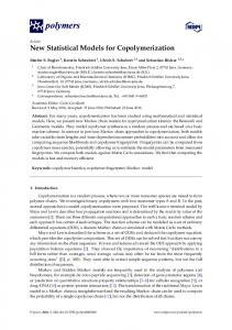
include Thomas Taylor who in 1877 suggested that friction ridges could be used to identify murderers, West Taber (1830-1912) who suggested in 1880 to use fingerprints to identify Chinese immigrant labourers since Westerners had problems identifying the population, and Gilbert Thompson (1839-1909) who in 1882 used an ink thumbprint impressed over the amount stated on the cheque to avoid fraudulent alterations. The 19th century also witnessed a number of important scientific works and publications that can be argued to have helped pioneer the use of fingerprint identification for widespread forensic purposes. A Czech physician Jan Evangelista Purkynˇe (1787-1869) discussed papillary ridges in a 1823 dissertation entitled Commentatio de examine physiologico organi visus et syjstematis cutanei (Cummins et al., 1940), in which he developed the earliest known attempt to create a taxonomy of different patterns (Cole, 2001), consisting of nine different fingerprint pattern types (Figure 1.2). Purkynˇe had studied the philosophy and built on Leibniz’s assertion that every natural object is unique to claim that no two individuals have the exact same fingerprint pattern detail.

Figure 1.2: The 9 fingerprint classes that Purkynˇe defined (images adapted from Cummins et al. (1940)). These are: (a) transverse curves (i.e. simple arch), (b) the central longitudinal stria (i.e. tented arch), (c) the oblique stripe (i.e., loop, ulnar, or radial), (d) the oblique loop (i.e., loop, ulnar, or radial), (e) the almond (i.e., whorl variant), (f) the spiral (i.e., whorl variant), (g) the ellipse (i.e., whorl variant), (h) the circle (i.e., whorl variant), (i) the double whorl.

Another important scientific publication in the 19th century was from Dr. Henry Faulds (1843-1930), who was a Scottish doctor located in Tokyo. He published a letter (Faulds, 1912) in 1880 in the scientific journal “Nature” in which he discussed fingerprints as a means of personal identification, and the use of printers ink as a method for obtaining such fingerprints from criminals. Faulds made comment to the permanence, classifiability, and uniqueness of fingerprints. He recorded fingerprints by spreading inked fingers evenly and thinly on a slightly damp paper sheet. Nonetheless, the most significant suggestion made by Faulds was that fingerprints could be used to solve crime via the retrieval of fingerprints from crime scenes. He even used greasy fingerprints to solve a petty crime 5

(Cole, 2004). However, the suggestion made by Faulds was given earlier in the July 1877 issue of The American Journal of Microscopy and Popular Science by the microscopist, Thomas Taylor, and it has been stated that the first forensic fingerprint identification may have been made as early as 1856 by John Maloy (Cole, 2004). Faulds, however, may have been the first to observe that fingerprint patterns have a tendency to be more similar amongst relations with the following cautiously worded statement: The dominancy of heredity through these infinite varieties is sometimes very striking. I have found unique patterns in a parent repeated with marvelous accuracy in his child. Negative results, however, might prove nothing to parentage, a caution which it is important to make.” Other key and arguably the most important scientific publications of the 19th century concerning fingerprint identification were produced by Sir Francis Galton in 1890-1891 (Galton, 1890, 1891a,b) and compiled in his 1892 book Finger Prints (Galton, 1892). This was the first scientific work that described and defined special ridge details, called minutiae, that are critical features for comparing fingerprints. Galton used the general pattern and minutiae features on eight pairs of fingerprints provided by Herschel from four adults taken 28 to 31 years apart, and two children taken nine and thirteen years apart, respectively, to evaluate the permanence of such features. Out of 296 defined minutiae points found to be usable for comparison, Galton found all to be matching between the respective pairs of impressions, while the general patterns also remained identical, further supporting the idea of permanence suggested by Herschel’s smaller experiment. He also devised a fingerprint indexing system for archiving and retrievals based on pattern classification and finger index (Galton, 1891a), inspired by the contemporary system A. Bertillon used to record and archive anthropometric measures (i.e. measures of physical characteristics such as height, scars, tattoos, and other skeletal/tissue landmark based measurements) in France. A second attempt was made in creating an index by incorporating the Bertillonage anthropometric system with the fingerprint classification method (Pearson, 1930). Finally, Galton made the first attempt to evaluate the strength of fingerprint evidence by deriving a simple statistical model based on empirical observations of general pattern frequencies and the occurrence of minutiae detail (see Section 2.1). The proposed statistical model supported the notion that fingerprints are individualised, as probabilities of repeated fingerprint ridge detail were orders of magnitude less improbable than the number of human fingerprints that ever existed. Several more 19th century key scientific works include literature by Paul-Jean Coulier (1824-1890), Arthur Kollmann (1858-1941), Hermann Klaatsch (1863-1916), Hermann Welcker (1822-1898), and Sir William J. Herschel (1833-1917). Coulier intended to use iodine vapours to detect document alterations but inadvertently discovered that latent (or hidden) fingermarks became visible using this technique. This was the first known development of latent fingermarks via chemical processes. Aubert repeated this technique in 1876 to detect latent prints. Kollman published a paper on primate hands and feet (Kollmann, 1883) discussing the embryological development of the ridges. He suggested that ridges are formed through lateral pressures between nascent structures and describes 6

how ridges discernible and fully formed for a foetus in the fourth and sixth month, respectively (Galton, 1892). Klaatsch researched the histology, ontogeny, and phylogeny of volar pads and friction ridges (Klaatsch, 1888). David Hepburn noted that that friction ridges increase the level of friction between the skin and the contacted medium, potentially assisting with holding the object (Hepburn, 1895, pp. 525-537). Welcker studied friction ridge permanence with an experiment using 1856 and 1897 prints of his right hand and published them both in 1898 (Wilder et al., 1918, pp. 341). Herschel (1916) observed that his own fingerprints taken in 1859, 1877, and 1916 had all the same ridge detail (Figure 1.3), signifying the possible permanence of friction ridge configurations. While this was a small sample set, it nonetheless may be the first known documented observation of fingerprint permanence (Figure 1.3).

Figure 1.3: Herschel’s right index and middle fingers impressed at 1859, 1877, and 1916. Figure sourced from Herschel (1916).

The 19th century can be seen as a pivotal century for the practical use of fingerprint identification in forensic investigations through key implementations of effective fingerprint classification techniques. Pioneers of such techniques included Juan Vucetich (1855-1925) and Sir Edward Richard Henry (1850-1931). Vucetich who was an Argentine anthropologist and police official created his own fingerprint classification system (launched in 1891) that stored criminal fingerprints and was the first system used by law enforcement personnel. His fingerprint training given to Police Inspector Alvarez of the Central Police is credited to have helped catch a murderer in 1892 (Ashbaugh, 1999) via fingerprint evidence (a bloody thumb print found on a door). This is often stated as being the first “concrete” example of a case solved by fingerprints. More identifications were to achieved, proving 7

fingerprints to be superior to anthropometry, which was evident when Argentina became the first country to abolish anthropometry in 1896 in favour of solely filing criminal records using only fingerprint classification. Henry developed a fingerprint classification system for use at his post as the Inspector General of the Bengali province in India. He had met with Galton in 1894 to learn what Galton had proposed for classification, which did not entirely solve all of the classification issues of practicality. Henry then collected ten-prints of all prisoners and successfully implemented a classification system. An independent assessment of Henry’s classification method in comparison to established anthropometry based methods was undertaken and concluded that his proposed method was simple, cost effective, centralised, rapid, and had proven results (Henry, 1900, pp. 67), resulting in the Indian government sanctioning the sole use of fingerprints for identification by 1897. After a favourable review by the Belper Committee, the Henry method for classification was later adopted in England in 1901, and later introduced in the USA in 1903 (Cole, 2001, pp. 137). The beginning of the 20th century witnessed the introduction of fingerprint evidence as admissible in courts of law throughout Europe, USA, and eventually, most jurisdictions worldwide. The first uses of fingerprint evidence include a burglary case in England (Lambourne, 1984, pp. 67-68) and a murder case for which Bertillon (1853-1914) made an identification. The inclusion of fingerprint evidence in courtrooms naturally lead to the requirements of a standard for comparing fingerprints and deciding whether a fingermark from a crime scene matches a given fingerprint of a suspect (see Section 1.2.4), and encouraged widespread collection of fingerprints from criminals in adopting jurisdictions. The 20th century also witnessed a continual nourishment of scientific knowledge and advancements in technologically centric applications.

Advancements in latent finger-

mark development include various chemical treatment techniques (Yamashita et al., 2011) that have been discovered to suit different environmental conditions and surfaces (i.e., porous/non-porous). Moreover, an greater understanding of the biological complexities of fingerprint formation and genetics has come to fruition, including a greater understanding of the formation and development of fingerprints in the womb (Cummins et al., 1943; Penrose et al., 1973; Bogle et al., 1994), and in general, the role that genetics play in determining the characteristics of fingerprints (Holt, 1961, 1968; Juberg et al., 1980; Kimura and Kitagawa, 1986). In addition, the modern age of computerisation and technological advancement allowed the introduced of the AFIS (see Section 1.2.2) for both law enforcement and border security applications along with biometric scanners that allow seamless electronically storage, quality assurance, and searching with AFIS. Other technological advancements include Mass Spectrometry UV imaging techniques enhanced with advanced image processing algorithms, and the development of improved data centric statistical models that predict the rarity of fingerprint features using data centric methodologies that could only have been made possible with the introduction of computationally based statistical tools and electronic datasets.

8

1.2

Fingerprint Identification

The modern application of fingerprint identification is based on research into papillary ridges that provides a scientific basis for the use of fingerprints for identification, advanced computing technologies that help expedite the identification process, and identification framework(s) and procedures that provide guidelines as to how accurate identification assessments by fingerprint experts can be achieved in practice.

1.2.1

The Scientific Basis of Fingerprint Identification

Ever since the scientific study of ridgeology began, pioneers such as Herschel (1916), Faulds (1880), and Galton (1892)), made the following axioms with regards to fingerprints: • uniqueness/discriminability: fingerprint features are deemed to be different for each individual,

• classifiable: the general pattern of the fingerprint can be categorised in a finite amount of well defined classes,

• immutable/unalterable: fingerprint features are not susceptible to change by natural or directed means,

• universality: the same well-defined fingerprint features exist in all individuals (however, with different configurations), and

• retrievable: fingerprint features from marks can be retrieved from the contacted medium,

all of which are crucial for applications of forensic identification. In particular, the axioms concerning the immutable/unalterable (or permanence) and uniqueness/discriminability of fingerprint characteristics requires a sound scientific basis in order to provide the high level of confidence for identification assessments that legal and law enforcement entities require. In general, the scientific basis for fingerprint identification must: • confirm the permanence of fingerprint characteristics • measure the rarity and variability of fingerprint characteristics • assess confidence measures for identification based on fingerprint characteristics • develop a method and process for comparing a crime scene latent mark to a known fingerprint template

in order to illustrate the scientific legitimacy of fingerprint identification (Cole, 2004). Whilst the first point strictly concerns fingerprint permanence, the second and third points are analogous with the rarity assessment of fingerprint features via the use of statistical analysis. In addition to establishing permanence and uniqueness of fingerprint features, a methodical framework must be used when forensic experts compare features between fingerprints, in order for identification claims to be as objective as possible. 9

1.2.1.1

Fingerprint Permanence

Fingerprint permanence describes both the immutable and unalterable nature of fingerprint features. The hypothesis of fingerprint permanence has been well supported in the scientific literature. Permanence was first studied prior to the early era of forensic fingerprint identification by Hermann Welcker (Wilder et al., 1918), who conducted a study from 1856 to 1897 (41 years) using his own right palm print. He found that both impressions appeared to be identical in detail. Other classical studies include Faulds (1880), Galton (1892), and most notably, Herschel (1916) who took the prints of individuals after 57 years, all of which supported the permanence hypothesis. More contemporary studies such as Okajima (1979), Wan et al. (2003), and Wertheim et al. (2002) have established that permanence is now a well established feature for fingerprints, where it is now known that a permanent modification of the ridge detail by physiological means can only occur via the destruction of the dermis layer of the skin. However, besides scarring and various skin conditions (David et al., 1970), there are other influences that challenge the permanence of fingerprint features. For example, advanced ageing causes surface ridges to flatten and the loss of elasticity in the dermis results in the skin to become flaccid (Okajima, 1979), ultimately causes the ridge pattern to become less visible. In addition, there have been reports of medication (particularly Capecitabine (Wong et al., 2009)) having a side effect of the removal of fingerprint ridge pattern detail. In general, modifications to fingerprints are likely to only occur from either prominent scarring, ageing, side effects of certain medication, or growth from infancy to adulthood (where generally, only isotropic rescaling is encountered (Gottschlich, 2011)). 1.2.1.2

Fingerprint Formation and Feature Rarity

Although a complete biological understanding of how epidermal ridge patterns form (Champod et al., 2016), some of the influential factors are well understood, while a number of possible mechanisms of formation have been proposed (K¨ ucken, 2007). Fingerprints are known to be fully formed at approximately seven months of foetus development (Maltoni et al., 2009). This includes genotypical along with phenotypical influences such as conditions in the womb, the flow of amniotic fluids around the foetus, the position of the foetus in the womb during the differentiation process of cells (Jain et al., 2002), and the temperature and pressure variability along with growth stresses encountered during embryonic formation. A hypothesis for exact minutiae development was provided by Hale (1952), where it was suggested that prior to primary ridges formation, cells proliferate to form clusters. These clusters then join together forming primary ridges. Ridge endings develop when a new ridge is formed between two existing ridges, whereas bifurcations are the result of ridge clusters developing on the side of a host ridge. Until now, there has been no strong evidence that supports this hypothesis. Some have suggested using pattern formation theories of mathematical biology (Kosz, 1999), who utilised this methodology to both model and compress minutiae detail, while other mathematical models of ridge and minutiae formation have been proposed in the scientific literature (K¨ ucken, 2007) based 10

on hypotheses regarding the physiological growth and development of fingerprints in the womb where a buckling process occurs in a cell layer of the epidermis. An indirect non-biological suggestion of configuration of minutiae uniqueness can be found in studies of monozygotic twins, who have identical DNA except for generally undetectable micro-mutations at cell division. While study found in (Okajima, 1979, pp. 660-673) indicates that a higher correlation exists for the number of minutiae present between the fingerprints of monozygotic twins in comparison to fraternal twins, other studies have demonstrated that the minutiae spatial configuration are still dissimilar enough to distinguish with algorithms (Jain et al., 2002). Another study has shown that while significant correlations for monozygotic twins in fingerprint class and ridge properties such as ridge count, width, separation, and depth (see Lin et al. (1982)) exists, variations in the minutiae distribution still permit their differentiation. In order to quantify the rarity of given fingerprint features, numerous statistical models have been proposed in the scientific literature. Since the first statistical model to measure the rarity of marked fingerprint features was proposed in Galton (1892) (see Chapter 2.2), some practical ambiguities have arisen from the study and development of the fingerprint uniqueness hypothesis. Such hurdles existing in the assessment of fingerprint rarity include: • real-world applications of uniqueness measurements- aspects that affect latent marks, such as noisy and partial information, making the creation of an accurate model for all possible real-life circumstances much harder, • non-trivial fingerprint feature modelling considerations such as fingerprint morphology,

• inter/intra-feature statistical dependency, • requirements for large samples of data for statistical rigour and accurate error rates, • well defined and agreed upon assessment and validation of a statistical uniqueness model.

Recent theoretical considerations in statistical methods have helped advance some of these modelling considerations (with such models discussed in Sections 2.2 and 2.3). In addition, the development of automated fingerprint systems such as AFIS (see Section 1.2.2) have helped with model data size considerations. Model assessment, however, has not been defined collaboratively or rigorously within the academic literature or by practitioners.

1.2.2

Automated Fingerprint Identification Systems (AFISs)

While the Henry system of classification improved the speed of searching and identification over the Bertillonage system (that was not primarily based on fingerprints), the establishment of large central repositories proved to be a practical restriction for a manual paper-based system. For example, after the formation of the FBI in 1924, a central fingerprint repository was created with an initial size of 810,188 records and had grown to 11

15 million records by the early 1960’s (Moses et al., 1979). Thus, there was a clear need for automation, in order to handle such large and ever-growing repositories. 1.2.2.1

Historical Developments

Automated Fingerprint Identification Systems (AFISs) leverage computer technology and advanced algorithms to store large quantities of fingerprint records in a database for the primary purpose of searching for potentially matching fingerprints against a submitted fingermark. The AFIS was first proposed in a patent filed in 1956 and published in 1960 (Maurer, 1960). Maurer described a method whereby fingerprint impressions can be positioned automatically by aligning lines that intersect the delta and the centre of the system of circular arcs near the tip of the finger (i.e., approximately the core point). Once aligned, scanning of eight or more defined regions is performed using an optical scanner from which a code can be derived from the electrical analysis of wave patterns to be ultimately used for the purposes of identification and classification (Figure 1.4). While the method described in the patent is not necessarily robust for real life scenarios, a feasible automatic procedure for image alignment and matching/classification was outlined.

Figure 1.4: (a) The line that intersects the delta and the centre of the system of arcs (i.e., roughly the core location) is suggested to be used to align fingerprints in the patent proposed by Maurer. (b) Suggested defined regions that can be analysed for matching and classification purposes after alignment is performed.

Another early theoretical discussion on the AFIS can be found from one of the earliest scientific publications that gave consideration to automated fingerprint identification (Trauring, 1963). Trauring made a proposal to automatically detect minutiae and authenticate fingerprints. Authentication was proposed by storing three non-collinear reference minutiae which are used to find the relative coordinates of a test minutiae location (within the triangle of the reference minutiae) using simultaneous equations, with the constants 12

used to solve the simultaneous equations then compared to determine if they are within a defined tolerance (to account for skin distortion and environmental changes). While this proposal was concentrating on authentication rather than 1:N matching, it was the first literature to propose using conventional fingerprint features (i.e., minutiae) for storing and matching. In the early 1960s, the FBI initiated a project to create an AFIS (Moses et al., 1979). The initial requirements for the practical development of an AFIS in the USA was defined by the FBI, in collaboration with NIST engineers. Their aims were to develop a fingerprint scanner that would automatically capture and electronically store inked prints, along with a system that would perform similarly to fingerprint experts by detecting and using minutiae to compare fingerprints. An RFQ (request for quotation) for a system to scan fingerprint images and detect minutiae was announced in 1966, where two successful proposals out of 14 responses were chosen. Concurrent to the development of fingerprint scanning and minutiae detection devices, a fingerprint matching algorithm was developed to compare two minutiae lists from two different fingerprint images and evaluate if minutiae details agree. After successful proposals for the fingerprint scanner, minutiae extracting, and fingerprint matching were demonstrated, new iterations were developed to cater for speed and accuracy, and by the late 1970s, the FBI were using these scanners to convert 15 million criminal fingerprint cards. While the FBI focussed on creating a solution for the general identification problem, during the 1960s and 1970s the UK Home Office, Paris Police, and Japanese National Police Agency were specifically interested in automating the matching of latent images against a master file of rolled prints. For instance, while the Paris Police developed minutiae matching hardware using an array of logical circuits and used a vidicon (i.e. video camera tube) to scan photographic film transparencies of fingerprints at 400 ppi, attempts were made to also develop special imaging techniques for high resolution imaging (such as FTIR) of live fingerprint images that is particularly suitable for latent work. The UK Home Office developed a fingerprint scanner that detected and recorded the position and orientation of minutiae, and was the first system to determine ridge counts to the five closest minutiae for each minutiae. The initial Japanese AFIS attempt was a semiautomatic classification and matching system based on a 17- to 20-digit manually encoded number that was an improvement on manual methods but still time consuming to manage and considered unsuitable for latent matching. In 1969, the National Police Agency of Japan asked NEC to develop a fully automatic AFIS using a minutiae-based methodology and collaborated with NIST in development of the AFIS. The NEC AFIS system was installed by 1982 and started the digitisation of fingerprint cards, while latent searches commenced a year later. Shortly after this, the NEC AFIS implementation (amongst other vendors such as Sagem Morpho from France) was subsequently implemented around the world in other jurisdictions, such as the National AFIS (NAFIS) in Australia. Following the early successes of the initial AFIS implementations, adoption had become widespread by the late 20th century. In 1999, The IAI AFIS directory of users counted 500 unique AFIS sites worldwide (IAI, 1999). Moreover, the range of applications for AFISs

13

has expanded to not only include law enforcement (for local, national, and international agencies), but in addition, military and civil field identification using portable technologies, border security and e-passports, national identity (such as in India, Brazil, Macau and South Africa), and even voting applications. The current state-of-the-art AFIS solutions provide near real-time responses and improved accuracy for fingerprint enrolment and identification, resulting from the advancement of feature detection and searching algorithms and computer processing/storage technologies. For example, the FBI AFIS contains the fingerprints of over 75.9 million subjects in the National Criminal History Record File and identified 25,955 fugitives in November 2013 alone, with millions of search requests submitted per year and an average response times in minutes (FBI, 2014). In addition, fingerprint scanning now consists of using live scan devices that are usually using optical scanning technology such as Frustrated Total Internal Reflection (FTIR) voiding the tedious need of preparing fingerprint cards with inked roll. Other recent advancements include 3-D based imaging techniques such as touch-less optical imaging and multi-spectral imaging. Such improvements have positioned the AFIS as a critical and effective system in support of law enforcement. 1.2.2.2

AFIS Functionality

The core functions of an AFIS are enrolment, quality assessment, verification (or authentication), and identification. The enrolment activities within an AFIS are as follows: • the enrolment of ten-print records consisting of all scans (of all available fingers for a known individual and typically includes biographical information of an individual

and meta-data for each finger (i.e., hand and finger position). This is achieved by using the images produced from a fingerprint scanner (often called live-scans) or scans of ink-rolled prints. • the enrolment of fingermark records (specifically for forensic applications) which consists of latent fingermarks that may or may not have a known origin.

• the ad-hoc live-scan enrolment of specific individual fingers. This typically is used in

non law enforcement based scenarios such as border access control or authenticationbased applications.

Each record of known identities within an AFIS database (also known as the Gallery) will often contain the associated images, available biographical information, and additional notes regarding the subject and/or samples. In addition, extracted features for each image will often be stored to aid the matching process within the AFIS or for the benefit of the fingerprint experts using the system. Such features can include the well-defined features of a fingerprint (see Appendix A) or algorithm-specific constructs specifically designed to be useful for indexing (for faster match results) and matching evaluations performed by the prescribed matching algorithm(s). Fingerprints used within AFIS often go through an automated quality evaluation via a quality assessment algorithm. Such quality algorithms can give ratings for individual 14

features within a template, along with an overall quality rating. Such quality assessments can be used in conjunction with AFIS core function workflows. For example, minimum quality criteria may be set for fingermarks to be enrolled or logical gallery groupings may be defined based on quality attributes. The task of verification is to perform a one-to-one (or 1:1) match evaluation of a query fingerprint against a prescribed template fingerprint record stored for a particular known individual. This task is primarily used for access control applications or for authenticationbased scenarios. In some cases, verification is performed against a few impressions of the same fingermark (i.e., 1:few evaluation). Identification involves conducting a search where a match evaluation is performed with a query fingerprint against each record in a gallery containing n fingerprint templates, in order to identify a source record. This is often termed a one-to-n (or 1:n) search. The most similar candidates from the gallery are returned in order of decreasing similarity (see Section 1.2.2.4). In the forensic context, AFIS identification consists of several different scenarios: • ten-print to ten-print matching- typically used to confirm an identity and/or consolidate duplicate records.

• known latent to ten-print matching- A known latent fingermark source can be confirmed against ten-print records or vice versa.

• unknown latent to ten-print matching- in the case of unknown latent fingermark

records, search requests against known ten-prints are usually performed in order to aid with with unsolved criminal cases.

Interoperability is another feature available for many AFIS implementations, where identification and enrolment requests are sent between AFISs of different jurisdictions. For example, the FBI’s Integrated Automated Fingerprint Identification System (IAFIS) provides law enforcement agencies with the ability to expand the search of latent fingermarks against a hierarchy of other regional, state, and national AFIS databases (FBI, 2014). 1.2.2.3

AFIS Matching Algorithms

Matching algorithms attempt to measure the similarity of features between two fingerprints. Both verification and identification tasks are dependent on this similarity measure. Algorithms define this similarity measure to quantify the amount of similarity or agreement of the features from one fingerprint against another. This metric is commonly called the similarity score or match score. The similarity score range and formulation is vendor and algorithm specific. The distributions of similarity scores for features discovered from impressions that come from the same source finger (denoted within-source comparisons) is generally centred around a higher mean value than score produced from features from different source fingers (denoted as between-source comparisons). 15

Largely speaking, there are fundamentally three different classes of fingerprint matching algorithms: • Correlation based- two fingerprint images are superimposed together with different displacement and rotations in order to calculate the maximal pixel-wise correlation.

• Non-Minutiae based- Sub-regional features other than minutiae/pores are used to

compare fingerprints. Such features based on properties of the fingerprint ridge patterns such as sub-region ridge orientation, frequency, shape, and texture information.

• Landmark based- Landmark features automatically extracted or manually marked

are used in a point-pattern matching problem. Such landmark features used are typically minutiae but can include level 1 relation features of cores/deltas and level 3 features such as pores). This algorithmic method is the closest to how the fingerprint expert will compare fingerprints.

Moreover, hybrid algorithms that combine different methodologies exist in order to improve the matching accuracy. 1.2.2.4

AFIS Candidate Lists

For each AFIS identification search request, the most similar candidates constitute what is called the candidate list. The candidate list is configured to contain a ranking of similarity scores in descending order. Candidate list entries are generally configured to be variable in size or being ranked within the top n results of the search, typically with all members greater than a score threshold. The AFIS matching algorithm ranks such correspondences in the candidate list by the matching score so that the highest scoring candidate has the highest rank which is often called the rank-1 candidate. The population of candidate list entries is considered to be close non-match (i.e., highly similar between-finger feature correspondences) or true match (i.e., highly similar within-finger feature correspondences) examples. In an ideal scenario where there is both qualitative and quantitative sufficiency of features to search on, a higher ranking for a candidate will correlate with a higher likelihood of being a true match correspondence (assuming that there is a match correspondence within the candidate list), ultimately helping the fingerprint expert expedite the identification process. 1.2.2.5

AFIS Matching Accuracy and Current Limitations

Several experiments have been run in order to assess the practical limitations that exists with regards to the accuracy of the AFIS matching technology. One such evaluation has been performed in the last several years by the National Institute of Standards and Technology (NIST) Evaluation of Latent Fingerprint Technologies-Extended Feature Sets (ELFT-EFS) with a main focus aimed towards comparing proprietary AFIS vendors on real-life performance of the matching accuracy for latent fingermarks (see Appendix A) using features marked by fingerprint experts and those automatically retrieved.

16

In a recent ELFT-EFS experiment (Indovina et al., 2011), five prominent commercial offerings of the current generation AFISs were tested for their rank-1 identification rate (i.e., what percentage of searches returned the correct individual with the highest similarity score). From observations of an experiment using 1114 latent fingermarks as the search set to be matched against 100,000 ten-print records (both rolled and flat scan instances for each record), some of the key following findings were noted: • For all AFISs tested, at least 20% of all fingermarks searches had a true matching template outside of the top 100 results in the resulting candidate list.

• From 112 fingermarks of which the human expert could not make a conclusive de-

termination, 8 were matched at rank-1 (i.e., candidate list entry with the highest score) and 31 were matched at rank > 100 by at least one AFIS matcher.

• The highest accuracy for all participating AFISs searched was observed when human expert marked features in addition to the fingermark images were used.

• The greatest portion of AFIS failed searches were for fingermarks with either a low number of minutiae and/or assessed by human experts to have poor image quality.

For fingermarks with fewer than 10 minutiae, human expert assessed quality was the best predictor of match accuracy. • Algorithm performance for fingermarks with 10 or more minutiae was highly and positively correlated to the number of minutiae.

• More than half of the fingermarks missed (approximately 22% of the dataset) by all matchers at rank-1 could be individualised by a human expert.

An updated evaluation (Indovina et al., 2012), was conducted where marginal improvement of accuracy was observed in most cases. Other notable findings from this evaluation were: • Matcher accuracy has a strong relationship with examiners’ prior subjective value determination assessments of Excellent, Good, Bad, Ugly, and No Value. The per-

formance of all matchers decreased consistently as lower quality fingermarks were searched. • The majority of fingermarks that did not return the correct result at rank-1 were of low minutiae count and assessed by examiners to be of poor quality or unusable.

• Matching algorithm accuracy (with regards to having the correct candidate positioned at rank-1) for all vendors was highly correlated to the number of minutiae in the query fingermark. • When the orientation of fingermarks was unable to be determined by an examiner, the rank-1 identification rates were substantially lower.

17

The findings of these evaluations suggest that, while AFIS matchers have high accuracy with good quality fingermarks that contain a substantial number of minutiae, lights-out systems (i.e., where no human expert intervention is involved in identification) are still not viable in many practical applications, particularly in the forensic context where poor quality and low number of minutiae often occur in fingermarks recovered from the crime scene (see Appendix A). On the other hand, AFIS matchers can occasionally correctly match fingermarks that human experts deem to be inconclusive. While the current generation AFIS cannot replace the human expert, they are certainly a valuable tool for identification purposes. An important practical consideration concerning the matching accuracy of all biometric systems concerns how a matcher performs with an increase in gallery size. In general, an increase in gallery size will result in both quantifiably and qualitatively more similar incorrect candidates returned from identification searches. This can potentially lower the rank of a true candidate or even remove it from the candidate list altogether, resulting in a lower identification rate. In the NIST Face Recognition Vendor Test (FRVT) (Grother et al., 2014), it was witnessed that the identification rates had a linear decrease for exponential growth of the gallery. Moreover, the decline in identification rate was more profound for biometric templates of lower quality. For example, an increase of gallery size from 160,000 to 1.6 million for the top performing matching algorithm resulted in an rank-1 identification rate drop of 0.5% and 2.9%, for mugshots (high quality) and webcam shots (lower quality), respectively. Considering that the gallery size used in the ELFT-EFS evaluation only contained 100,000 ten-print records, larger AFIS systems such as the Australian NAFIS (Anon., 2016) or the FBI IAFIS that contain over 6.7 million and 72 million ten-print records, respectively, illustrate how real-world applications have much larger search galleries. Moreover, they generally only contain rolled or flat scan impression, not both variants for each record. This signals that the limitations discovered in the ELFT-EFS may be exacerbated in real-world applications due to ever-increasing gallery sizes and collection practises.

1.2.3

ACE-V Identification Methodology

The identification process involves the expert determination on whether a query fingermark (typically retrieved from the surface of an object from a crime scene using developmental processes) comes from the same source finger (and thus, individual) that impressed a reference print. In an attempt to assess identification in a consistent and accurate manner, fingerprint experts use a peer-review based methodology known as ACE-V (Analysis, Comparison, Evaluation, Verification) (SWGFAST, 2002, pp. 2), as originally developed by the Royal Canadian Mountain Police (RCMP). This acronym describes an order of key steps taken during the identification process (Champod et al., 2016; Ashbaugh, 1999). • Analysis: The Analysis stage consists of an assessment of the fingermark with regards to the level of detail present (see Appendix A). Level 1, 2, and 3 friction ridge features

useful for identification that are found in the fingermark annotated by the fingerprint expert. Each of the three levels of features is recorded without any prior assessment 18

of the selectivity of the features, in order to uphold objectivity. Following this, a decision is made as to whether the quality and amount of detail present within the fingermark is sufficient to perform an identification. The fingerprint expert will make such a determination based solely on their expert opinion, which is based on training and previous experience. If the fingermark is deemed insufficient for comparison, the ACE-V process does not continue any further. • Comparison: If the fingermark is deemed sufficient in the Analysis stage, the next stage that is performed is Comparison. The Comparison stage involves the direct

comparison of friction ridge detail of the fingermark with the detail found within a reference fingerprint or fingermark (which is assumed to have friction ridge details also annotated and deemed useful for identification, prior to this identification attempt). The successive comparison of level 1, 2, and 3 features is performed, where features are compared for categoric and spatial consistency, with regards to their ridge path sequence and occurrence. Categoric consistency concerns the consistency of feature class or type such as fingerprint pattern class, minutiae type, and pore type. Spatial consistency concerns the spatial measurement of scaled distances between corresponding landmark features and the appearance of shape, accounting for variation due to skin elasticity, impression force, contacted medium, and other environmental factors. The disagreement of features include any categoric or spatial inconsistencies, along with the non-correspondence of features. However, the disagreement of features may be logically compatible with a positive identification. For instance, missing features may result from poor quality and/or variable fingermark coverage, whereas spurious features may result from environmental conditions. In addition, categoric inconsistencies such as minutiae and pore type may also result from similar factors. The examiner should avoid any prior knowledge of examination and should be focussed primarily on features that have been identified in the previous analysis step. This will ensure that objectivity is maximised during the comparison process. Finally, the outcome of the comparison process should result in a charted comparison between the two images, emphasising concordances and differences between the fingermark and reference mark/print at all three levels of features. • Evaluation: The Evaluation stage follows the Comparison stage, where a preliminary identification conclusion is made. A possible outcome of individualisation, exclusion,

or inconclusive is made by the fingerprint expert. While the fingerprint expert will use the deductive reasoning of the agreement/disagreement of compared features, the identification inference requires an opinion-based decision as to whether there is a significant level of correspondences or disagreement of features, while taking into account the quality of such features. This expert decision is based on either the training and experience of the practitioner or predefined guidelines that provide a numerical rule (see Section 1.2.4) for the number of corresponding features required to make a positive identification.

19

• Verification: This verification stage is is a peer-review process, where all prior ACE

stages are repeated by another expert who has no prior knowledge of the analyses and conclusion made by the original examiner. The two identification conclusions are verified for consistency. If consistency is not found, a conflict-resolution process is performed.

The possible outcomes of the ACE-V process are as follows (Lennard, 2013): • Individualisation- there are sufficient features in agreement to conclude that the two

areas of friction ridge impressions originated from the same source and the likelihood that the impression was made by another source is so unlikely that it is considered as a practical impossibility,

• Exclusion- there are sufficient features in disagreement (i.e., unexplained by variations caused by skin distortion or environmental noise) to conclude that the two areas of friction ridge impressions did not originate from the same source finger, and • Inconclusive- the corresponding information in the latent and exemplar fingermarks is inadequate to permit a conclusion. Typically, the examiner provides no additional

information regarding the chances that the two prints did or did not share a common source. Such outcomes based on the ACE-V process and expert opinion are presented in the courtroom as admissible expert evidence. 1.2.3.1

ACE-V and AFIS Searches

The ACE-V framework is often used in conjunction with AFIS. Figure 1.5 outlines the flow chart of how the stages of ACE-V and AFIS interact with each other. Using the marked features found in the Analysis stage of ACE-V, the fingerprint expert can perform a search on the AFIS which will return a candidate list of the most similar fingerprints (as deemed by the AFIS matching algorithm). This allows the fingerprint expert to avoid the impossible task of manually comparing a fingermark with a large number of fingerprints in an archive. Instead, a comparison with the small number of entries within the candidate list is only required.

20

Figure 1.5: Flowchart of modern ACE-V process used in conjunction with AFIS. The iterative comparison of each exemplar fingerprint in the AFIS candidate list (i.e., most similar records in an AFIS database ranked by order of similarity) is performed until identification occurs or no more exemplars are left. The red flow lines indicate the process for the verification stage analysis. The purple flow line from the ’agreement of features’ test shows the ACE process that skips the evaluation stage.

1.2.4

Forensic Fingerprint Identification Standards

Since the early use of fingerprints in forensic identification, practitioners have been required to essentially make a boolean decision on whether they believe a latent mark(s) match a template mark or print(s). No matter what statistical basis or lack thereof, the fundamental question that must be asked is how can we vouch for the conclusion that two impressions are derived from the same source print (Cole, 2004)? This question is of direct consequence to the evaluation stage of the proposed ACE-V framework. Historically speaking, Galton and Forgeot were the first to try and articulate a match process (Cole, 2004). Forgeot suggested using enlarged photographs of the two impressions while tracing ridge lines for enhancement. A determination was then to be made on each enlarged photograph with the added traces. Galton focussed on a more systematic methodology, marking minutiae locations on both prints and attempted to match minutiae locations (Galton, 1892). Of both methods, Galton’s method was more widely documented in early use (Henry, 1900; Olsen, 1988). The application of Galton’s method for identification raised the question of how many 21

minutiae are required for a match. Initially, early practitioners relied on their intuition and personal experience. While Galton created a probabilistic model based on local ridge analysis (see Section 2.2.1.1), no identification framework was proposed. Other probabilistic models were also formulated soon after (see Section 2.2.3.2) with no interpretive framework for application to identification. 1.2.4.1

Balthazard’s Numerical Standard

Using a probabilistic model (see Section 2.2.3.2) and taking into account the human population at the time (1.5 billion), Dr. Victor Balthazard (Balthazard, 1911) was the first to provide a numerical standard, suggesting that a minimum of 17 corresponding minutiae would be needed to identify an individual with certainty. However, Balthazard also suggested that this number could be reduced if the suspect population in question was limited to a town or country. 1.2.4.2

Locard’s Tripartite Rule

In 1914, the French criminalist Edmond Locard (Champod, 1995) made the earliest concise attempt to provide an identification framework called the Tripartite Rule, where the weight of evidence for identification is described as a continuous (rather than a boolean) determination of the sufficiency of evidence for identification. The determination of sufficiency encompassed a probabilistic component for insufficient or inconclusive evidence, along with a numerical standard for evidence deemed sufficient for a conclusive identification. The Tripartite Rule is described as follows: • Positive identification is possible with more than 12 minutiae if the fingerprints are sharp (i.e., high quality).

• If 8 to 12 concurring points are involved, then the case is borderline and the certainty of identity will depend on quality of prints, rarity of pattern, presence of core and

deltas, presence of pores, width of the papillary ridges and valleys, and directions of minutiae and ridges in general. In these cases, certainty can only be established by at least 2 fingerprint experts. • If a limited number of characteristic points are present, the fingerprints cannot provide certainty for an identification, but only a presumption proportional to the number of points available and their clarity (i.e., probabilistic value). The tripartite rule proposes a framework for fingerprint identification that includes all levels of detail. Taken in a holistic sense, the tripartite rule can be seen as a probabilistic framework, where the successful applications of the first and second rules are analogous to a 100% probability that impressions are from the same sources, whereas the third rule covers the probability range of 0% to 100%.

22

1.2.4.3

Adoption of a Numerical Standards

Locard’s first rule of imposing a numerical lower limit for a positive identification became standard practice for many jurisdictions worldwide, and is still used to some extent in conjunction with the ACE-V framework (i.e. for the evaluation stage). Currently, the majority of European fingerprint experts favour a purely quantitative approach (see Champod et al. (2016)), prescribing a fixed numerical standard. For example, Belgium, Finland, France, Greece, Ireland, Israel, Poland, Portugal, Romania, Slovenia, Spain, Turkey, Japan, and countries within the South Americas, are examples of countries who adhere to the 12-point rule. Other jurisdictions employ rules based on combinations of Locard’s first and second rules (for example, Germany, Sweden, Holland, and Switzerland). Other jurisdictions have used more conservative numerical standards than Locard’s Tripartite Rule had prescribed. Italy adopted a 16-17 point rule prescribed from the studies of Balthazard (Champod et al., 2016), while the UK had adopted a 16 point rule largely due to Alphonse Bertillon’s published article where he constructed two different fingerprints from fragments of other fingerprints, resulting in both artificial fingerprints loosely having 16 minutiae in agreement (Cole, 1999). This led to the UK adopting a more conservative 16 point rule in 1924, that was used as a mere recommendation for identification before the 1950s. However, following cases in the early 1950s where correspondences of up to 15 minutiae were discovered from fingermarks of different sources (Champod et al., 2009), this numerical standard was applied more rigorously in future identifications. Since 2001, the UK has adopted a non-numeric holistic approach. 1.2.4.4

Holistic Approach

The have been questions regarding the scientific reasoning of a numerical standard. By the 1950s, American fingerprint examiners were questioning having a minimum numerical standard for a positive identification, suggesting that the number of matching points may not be an accurate determination of rarity (Cole, 2001, pp. 261). In addition, the precision implied by having a numerical standard encourages the fingerprint expert to more readily identify minutiae as being sufficient for comparison in order to reach the magic number for identification (Champod et al., 2016, pp. 45). In the IAI 1973 resolution IAI (1973), the committee stated that ...no valid basis exists at this time for requiring that a pre-determined minimum number of friction ridge characteristics must be present in two impressions in order to establish positive identification”. A number of jurisdictions, such as Australia, U.K, and U.S.A, subsequently adopted a what is termed a holistic approach (Champod et al., 2016), where no strict numerical standard or feature combination is prescribed. Thus, the forensic examiner in such jurisdictions will heavily rely on their expertise and experience to make an identification assessment. Since the holistic approach attributes identification assessments with a direct dependence on the examiner’s expert opinion (rather than a dependence on predefined numerical guidelines), a strong push for training and certification followed within the forensic community. For 23

instance, the IAI formulated a certification program to ensure competency and accuracy in identification (Cole, 2001, pp. 264). However, at the time, some within the forensic community insisted that the certification did not provide total protection against error. 1.2.4.5

Probabilistic Approach

Locard’s third rule, which involves a higher degree of probabilistic interpretation of evidence, had not been historically popular and was even banned by professional bodies (see Champod (1995)). The International Association of Identification’s (IAI) Scientific Working Group on Friction Ridge Analysis, Study and Technology (SWGFAST), made an official statement (see SWGFAST (2002)) which eliminated the use of probabilities in conclusions of latent mark comparisons. In addition to this statement, previous IAI resolutions have weighted heavily against a probabilistic frame work. For instance, the IAI Resolution 1980-5 stated: “THEREFORE BE IT RESOLVED that any member, officer or certified latent print examiner who initiates or volunteers oral or written reports, or testimony of possible, probable or likely friction ridge identification, or who, when required in a judicial proceeding to provide such reports or testimony, does not qualify it with a statement that the print in question could be that of someone else, shall be deemed to be engaged in conduct unbecoming such member...” There are no known jurisdictions that use any formal probabilistic methodology for identification assessment. However, in recent times, statistical models have been given more favourable treatment for real-world forensic applications. It was suggested in Champod et al. (2001) that a probabilistic framework is, philosophically speaking, based on stronger scientific principles than current numerical standards. In addition, the IAI rescinded the ban on reporting possible, probable, or likely conclusions (see IAI (2010)) and allowed the use of mathematically based models accepted as valid by the relevant scientific community to assess the associative value of the evidence.

1.3

Criticisms of Fingerprint Identification

Until recently, fingerprint identifications had near unanimous acceptance as robust forensic evidence, where testimonies provided by fingerprint experts were deemed as sound scientific evidence admissible in court, while the methodologies and philosophical foundations crucial to the task of identification were generally accepted as ground truths. However, there have been a number of recent criticisms made concerning the scientific validity of forensic fingerprint identification (Saks, 2010; Cole, 2008; Koehler et al., 2010; Haber et al., 2008). Such criticisms made by commentators concern the philosophical premises of fingerprint identification, the lack of scientific quantification used in identification assessments, the ACE-V process, and the lack of understanding of contextual bias.

24

1.3.1

Admissibility of Scientific Expert Testimony

It has been reported that fingerprint evidence is presented in approximately 28.5% of cases that include some form of admissible evidence (Cole, 2005, pp. 1071). In the 1993 case of Daubert v. Merrell Dow Pharmaceuticals (Anon., 1993) a ruling of significant importance by the Supreme Court in the United States, was made that outlined criteria concerning the admissibility of scientific expert testimony, based somewhat on criteria used in the broader scientific community. The criteria for a valid scientific method were given as follows: • must be based on testable and falsifiable theories or techniques, • must be subjected to peer-review and publication, • must have known or predictable error rates, • must have standards and controls concerning its applications, and • must be generally accepted by a relevant scientific community. The guidelines for expert testimony admissibility from Daubert have since influenced international jurisdictions, with the UK Law Commission’s recent expert evidence consultation paper (Anon., 2011) also prescribing similar standards (with an emphasis on scientific method more so than falsifiability). The recent wave of criticisms in North America have often referenced the Daubert decision (Page et al., 2011). Criticisms made from a number of academics and legal commentators have cited the following objections (Haber et al., 2009): • the cognitive biases of experts for decisions made within the ACE-V framework, • the unfounded and unfalsifiable theoretical foundations of fingerprint feature discriminability and uniqueness, and

• the ‘unscientific’ absolute conclusions of identification in testimonies (i.e., either identification, exclusion, or inconclusive).

While cognitive biases are primarily concerned with influences on the integrity, accuracy, and consistency of practitioners within the ACE-V process (Langenburg et al., 2009; Hall et al., 2008; Dror et al., 2011), the remaining criticisms can be restated as the non-existence of a scientifically sound probabilistic framework for fingerprint evidential assessment, that has the consensual approval from the forensic science community.

1.3.2

Erroneous Identifications

One of the key antagonists for the recent criticisms of fingerprint identification is a number of key well-publicised erroneous identifications that have been made over the last couple of decades. Such erroneous identifications have raised questions with regards to the identification accuracy of fingerprint experts within the ACE-V framework. Some recent examples of high-profile erroneous identification cases that have often been cited by critics of fingerprint identification include Shirley McKie and Brandon Mayfield. 25

Figure 1.6: The contentious 16 points used to identify the latent mark retrieved from the Marion Ross murder crime scene (top) against Shirley McKie’s template mark (below). Images sourced from German (2015). In 1997, David Asbury was convicted of the murder of Marion Ross. However, in the course of the investigation, a fingerprint (Figure 1.6) was found on the bathroom door frame that was identified by officers of the Scottish Criminal Record Office to belong to a police officer, Shirley McKie, who denied that she was ever inside that area of the crime scene. Shirley McKie was prosecuted for perjury in the case HM Advocate v. McKie. However, during her trial, defence fingerprint experts noted that an erroneous identification had taken place, where it was clear that the latent mark was not from Shirley McKie. In fact, two independent experts (Cole, 2001) were reported to recognise the error explicitly, where one expert noted that the error was obvious and that it could be recognised in seconds (Jayaprakash, 2013). Shirley McKie was subsequently found not guilty of perjury. In 2004, Brandon Mayfield was involved in one of the most highly publicised erroneous fingerprint identifications (Cole, 2005; OIG., 2006). Following the Madrid train bombings, a senior fingerprint examiner from the Federal Bureau of Investigation (FBI) 26

identified Brandon Mayfield’s template print from an AFIS search against the latent mark recovered from a bag found containing detonators and explosives. Mayfield’s prints had been taken earlier due to both his military service and his arrest for burglary in 1984. The identification was verified by the supervisory fingerprint specialist, and Mayfield was subsequently arrested and held in custody. A third independent well-known fingerprint examiner testified that while the comparison was quite difficult, the claimed identification was correct. Soon after, the Spanish National Police found their own identification (Ouhnane Daoud, an Algerian national living in Spain; Figure 1.7), while it was apparent that Mayfield did not have a passport to travel overseas, causing the FBI to retract the claimed an identification and issue an apology.

Figure 1.7: (left) The latent mark retrieved from the crime scene with 10 minutiae (out of the 15 marked features) used for the erroneous identification. (centre) Ouhnane Daoud’s exemplar correctly identified by Spanish Police. (right) Brandon Mayfield’s exemplar erroneously identified by the FBI (OIG., 2006, pp. 132-134). Some other notable erroneous identifications that have occurred in the last few decades include: • In 1982 the American case State v. Caldwell a murder conviction in 1977 was reversed due to an erroneous identification by the prosecutors IAI certified fingerprint expert. The erroneous identification was incorrectly confirmed by another certified expert in the defence team. The fact that both experts were certified raised questions within the community with regards to human error, the standards of certification and training, and the holistic approach of identification that heavily relies on the expert’s opinion. • In 1997, Scotland Yard’s fingerprint examiners had erroneously matched a print from a burglary crime scene to a suspect, Andrew Chiory. Failure of a proper

peer review of the examiner’s claimed identification was noted as the cause for the misidentification.

27

• In 1998, the British court freed Danny McNamee (Cole, 2001) who was convicting for a suspected Ireland Republic Army terrorist attack in 1982. An appeal was made,

where 14 expert witnesses disagreed on the value of the fingerprint evidence. Some stated that the print had too poor quality for an identification, while others who made a positive identification could not find the 16 points of similarity (as the U.K. standard at the time advised). • In 2004, Lana Canen was arrested and charged with the 2002 murder of Helen Sailors

based on fingerprint evidence. Lana Canan was later convicted in 2005. In 2011, an independent fingerprint examiner was hired to re-examine the fingerprint evidence, who found the identification to be erroneous. After the Indiana State Police Crime Lab verified this error, Lana Canen was subsequently released from prison in 2012.

A more detailed list of past erroneous fingerprint individualisations has been provided by Cole (2005).

1.3.3

Fingerprint Expert Accuracy under ACE-V

Such well-publicised erroneous identifications have raised questions with regards to the error rates of fingerprint identification by practitioners within the ACE-V framework. In response, there have been a number of studies attempting to quantify the error rates of identification with ACE-V and trained fingerprint experts. In an extensive experiment performed by Ulery et al. (2011), 169 fingerprint examiners each compared approximately 100 pairs of latent and exemplar fingermarks from a pool of 744 pairs. The false positive rate for ACE (ACE-V without the verification stage) was 0.1%, while the inclusion of verification resulted in all false positive errors being detected. Another study (Wertheim et al., 2006) examined the accuracy of fingerprint examiners during comparison training exercises, with 92 examiners having over one year experience having an erroneous identification rate of 0.034% (ACE only). Finally, another large scale study (Pacheco et al., 2014) was recently conducted where 108 fingerprint examiners were each given 80 pairs of fingermarks/exemplars of varying quality to assess for identification, while participants were able to reproduce a correct identification 94.2% of the time and not reproduce an erroneous identification 100% of the time.

1.3.4

ACE-V and Cognitive Bias

In the general forensic science context, cognitive bias may affect the analysis and decision making of a forensic expert. Critics have often cited cognitive biases as a real problem in practice, as the forensic expert (despite his or her training and methodology) will perform subjective assessment and comparisons stages that are potentially susceptible to unconscious personal bias, which in turn could undermine the objectivity and impartiality of the forensic process. Two closely related forms of cognitive biases that are often discussed are confirmation and contextual bias (Dror, 2009). Confirmation bias is where the expectations of the forensic expert affects how analysis and interpretation of evidence may be performed (Kassin et al., 2013), where confirming 28

rather than disconfirming evidence is the focus. The internal investigation by the FBI (OIG., 2006, pp. 144) stated that confirmation bias was listed as a contributing factor to the erroneous identification (Figure 1.8). Furthermore, it has been suggested that confirmation bias may play a part in the practice of fingerprint practitioners revisiting the initial marked minutiae detail of a fingermark in the analysis stage, once comparison with an exemplar had commenced. In Ulery et al. (2015), an experiment involving 170 examiners, each randomly assigned 22 pairs of prints from a pool of 320 total pairs, had their identification evaluations documented. It was noted that when positive identifications were claimed, a high rate (90.3%) of adding or deleting minutiae from what was originally marked in the analysis stage occurred, while inconclusive and exclusion determinations had a lower rate of revisiting. In close relation to confirmation bias, contextual bias concerns the influence specifically by extraneous contextual information on analysis and identification. In the ACE-V context, contextual bias is the influence by extraneous contextual information that fingerprint experts encounter in decision making during all stages of identification (Langenburg et al., 2009). Critics have argued that contextual bias is a real problem for the integrity of the criminal justice system, citing how in real-world scenarios, forensic experts are exposed to contextual information that is not necessary for their analysis work (Edmond et al., 2015). Furthermore, contextual bias has been demonstrated to affect the interpretation of forensic evidence, potentially undermining the value and admissibility of expert evidence.

Figure 1.8: (left) Brandon Mayfield’s exemplar erroneously identified by the FBI with 5 minutiae not existing in the latent mark. (right) The latent mark retrieved from the crime scene with the 5 missing minutiae positions overlayed (OIG., 2006, pp. 140-141). To further understand the effects of contextual bias on the accuracy of forensic fingerprint identification evaluations, there have been a number of studies concerned with contextual bias and the associated error rates of ACE-V evaluations in practice. The studies of Dror et al. (2006) and Langenburg (2009) suggested that repeatability (and repro-

29

ducibility) of identification results are correlated with the quantity, clarity, and specificity of ridge detail. The experiments reported by Langenburg et al. (2009) led to conclusions that experts appear more susceptible to bias assessments of ‘inconclusive’ and ‘exclusion’, while false positive rates are reasonably low within simulation of the ACE-V framework. It has also been suggested from results reported by Hall et al. (2008) and Schiffer et al. (2007) that not all stages of ACE-V are equally vulnerable to contextual bias, with primary effects occurring in the analysis stage, with proposals on how to mediate such variability found in Dror et al. (2011). Finally, the study by Pacheco et al. (2014) noted that under biased conditions, participants, in general, were able to reproduce a correct identification 73.0% of the time and not reproduce an erroneous identification 96.5% of the time. Furthermore, participants were able to repeat their previous correct identifications and previous erroneous exclusions 93.2% and 85.2% of the time, respectively.

1.3.5

Individualisation, Uniqueness and Discriminability

Generally speaking, the primary goal for forensic identification disciplines is to produce conclusions of individualisation, where the reduction of the donor pool is focussed towards a single source. While forensic science has at the very least illustrated a high discriminability of feature and characteristics of certain trace evidences such as fingerprints, critics have often questioned the scientific basis of individuality claimed by forensic practitioners, pointing out the absurdity of claiming such an unprovable notion (Page et al., 2011). In summary, the argument against the concept of individualisation can be summarised as (Saks, 2010; Kaye, 2010): • Individualisation exists only in a metaphysical sense, having no scientific validity, and it is supported largely by faulty logic that equates infrequency with uniqueness.

• The probabilistic approach always leads to the conclusion that a source other than

the suspected individual or object might exist, since there is always a probability greater than zero. In addition, the product of probabilities greater than zero always yields a value greater than zero. This is referred to by some as the product rule (Tijms, 2012).

• Uniqueness claims cannot be proven without a complete set of samples (i.e., ev-

ery human being past, present, and in the future have to be checked to determine if uniqueness exists). Anything less results in probability statements rather than conclusions of absolute specificity and absolute identification.

• Following the philosophy of Karl Popper, it is logically impossible to prove a hypothesis by accumulating a finite subset of positive examples. One must consider the total population of humans ever to have lived, in addition to the number of people yet to be born, in order to assert that a particular characteristic is truly unique. • Forensic experts across disciplines have made no systematic, concerted effort to find different objects that produce identical traces. 30

In the fingerprint identification context, the core axiom of fingerprint feature uniqueness, which was suggested in the early period of fingerprint identification by pioneers such as Galton and Locard, is still accepted by fingerprint experts today. In fact, some fingerprint experts have stated that the uniqueness of fingerprint features exists right down to the level of a single ridge: The fact is, a single ridge is unique. Therefore, anything comprised of multiple units of something unique must also be unique. Many use the reverse argument, which is just as valid...if a whole fingerprint is unique and you cut it in half, it is still unique. There is no such thing as “half” of unique. Unique is unique (Cole, 2009, pp. 12). While the uniqueness axiom has some biological and experiential/observational merit that some would claim goes beyond simple anecdotal evidence, on a philosophical level, uniqueness of fingerprint features cannot be proven, for the very same reasons as given by Saks (2010). That is, not all fingerprints have been compared with each other, nor is there any mechanism that guarantees a timeless uniqueness of fingerprint features (McLachlan, 1995). Some critics have invoked this traditional interpretation for the observed discriminability of fingerprint features (Saks et al., 2008; Cole, 2005), claiming that an assumption of ‘uniqueness’ is still used by forensic scientists and practitioners today, since it is often the case that experts employ absolute conclusions of identification in their testimonies. In response to such philosophical criticisms of the traditional view of fingerprint feature uniqueness, more and more forensic experts and legal commentators have disassociated discriminability from uniqueness (Kaye, 2010). Some have claimed that ”uniqueness is not relevant to the theory or practice of forensic identification, or to the courts, and that individualisation is the task of the judge or jury” (Page et al., 2011, pp. 17). Others have suggested that critics who believe that no probability of duplication is small enough to warrant an opinion that forensic evidence is unique are mistaken. For example, given a total of n fingerprints in the world, while the probability of two fingerprints being the same is some unknown value

1 m,

then the probability of finding at least two fingerprints

with identical features (using the Birthday Paradox) is $

1 P (n) = 1 − 1 − m

%

$

2 × 1− m

%

& n' × ... × 1 − . m

(1.1)

Thus, if the fingerprint expert can deduce a probability representing the rarity of the given corresponding features that is several orders of magnitude lower than this hypothesised probability, then practically speaking, this is enough to infer an individualisation, despite the probability being greater than zero. This inference is not the hypothetical inference suggested by the critics of individualisation that demands the probability equal zero, but rather, is a practical inference. In response to this argument, commentators state that this reasoning still appears contrary to the uniqueness hypothesis, that specifically implies that there will never be a repetition of the same arrangement of friction ridge characteristics (Page et al., 2011). Commentators who have stated that opposition to uniqueness assumptions and indi31

vidualisation claims have also suggested that fingerprint and other forensic identifications who espouse to such fundamentals can survive without the uniqueness hypothesis, by reformulating the conclusions drawn to include an empirically testable Bayesian framework (Cole, 2009). Such proponents often cite DNA profiling as an example of forensic science that already does not use the individualisation principles. In addition, DNA profiling is regarded as having both a probabilistic framework and transparency with regards to methods used.

1.4 1.4.1

Statistical Models and Identification The Need for Statistical Models

The criticisms based on the Daubert admissibility test (see Section 1.3.1) concerning (i) unfalsifiable theoretical foundations of fingerprint feature discriminability and uniqueness, and (ii) the ‘unscientific’ absolute conclusions of identification in testimonies have brought into question the fundamental theoretical foundations behind fingerprint identification. Fingerprint experts have been accused of dogmatically adopting the traditional axiom of uniqueness of fingerprint features for real-world identification scenarios, where the merit of such criticisms are strengthened, due to the fact that fingerprint features used in identification are usually sparse and have added uncertainty caused by noisy environmental factors that affect their visual clarity. Criticisms relating to the axiom of fingerprint uniqueness can be restated as the nonexistence of a scientifically sound probabilistic framework for fingerprint evidential assessment that has the consensual approval from the forensic science community. Currently, there is no generally accepted statistical model. However, the fingerprint identification practice is receiving increasing pressure to perform such fundamental research concerning the uniqueness of fingerprints and to develop and employ statistical models that could be used to present fingerprint evidence in court. It can be argued that the growing concerns and criticisms of fingerprint identification have initiated a number of recently proposed statistical models that aim to accurately model and predict the discriminability (or rarity) of fingerprint features used commonly in identification. Some models (Zhu et al., 2006; Su et al., 2010; Lim et al., 2011) focus solely on calculating the probability of obtaining corresponding features from different finger sources (often termed as the Probability of Random Correspondence, abbreviated as PRC), whereas others (Egli et al., 2007; Egli, 2009; Choi et al., 2011; Neumann et al., 2006, 2007, 2012) focus on calculating an evidential weighting of a given feature configuration using likelihood ratios. The latter model variant provides a more practically driven approach for supporting identifications, as both within-finger and between-finger feature correspondences are analysed. In further support of statistical models, relevant bodies within the forensic community such as the European Fingerprint Working Group (EFPWG) (Meuwly, 2011) and the International Association for Identification (IAI) (IAI, 2010) have expressed their approval for the use of statistical models. However, the IAI stated that a statistical model should 32

not be used as the sole determinant, but rather an aid for evaluation. Guidelines on how to include statistical methods in evaluative reporting have been provided by ENFSI (Willis et al., 2015). Research into the use of statistical models to calculate fingerprint probabilities is ongoing and small-scale trials of fingerprint identification using statistical models as a support tool for the examiner have been undertaken (Langenburg et al., 2012), but, as yet, a model has yet to be officially endorsed by any forensic identification body for use in casework.

1.4.2

Identification Conclusions and Statistical Models

One of the aims of recent research is to develop and employ statistical models that could potentially be used to present fingerprint evidence in court. Some commentators (Cole, 2009) have cited DNA evidence as an example of a forensic discipline that successfully follows a modern scientific framework, where DNA profiling is based on statistical methods that have probative results transparently presented as expert testimony, with a reluctance to give an expert opinion or interpretation of the result (Lennard, 2013). In comparison, the current situation for fingerprint discipline contrasts that of more recent forensic disciplines such as DNA, where fingerprint testimony is based on conclusive opinions that are made with no accepted statistical model to back up these opinions. The proposal to use probative information from such models in fingerprint expert testimony has presented differing opinions within the discipline and broader forensic science and legal communities. Some have questioned the need to change the current testimony format for identification to be strictly probabilistic as it is with DNA, citing the following reasons (Lennard, 2013): • While organisations such as the IAI are now in favour of statistical models, a condition was to use models that are formally endorsed and authorised by the scientific community. However, model development can be argued to be still in an early stage of development. In addition, currently no ubiquitously endorsed model exists. • Most inconclusive comparisons involve fewer than 8 corresponding minutiae. Given the current high error rates of existing models with less than 8 minutiae, many erroneous identifications and exclusions will result. • Currently, there is research being undertaken that will perform automated identification using AFIS algorithms. This ‘lights out’ is likely to be used for non-complex

identification and exclusion cases. This will leave the remaining complex cases for the fingerprint examiner to review. To employ statistical models for such complex cases may increase the risk of error. • As fingerprint databases get larger, the probability of finding close non-matches (i.e., minutiae correspondences from different finger marks) increases. Such a scenario places a heightened importance for statistical models that focus specifically on the candidate list population (i.e., close non-matches versus true matches). Few statistical models specifically focus on such a targeted population. 33

• Since the probabilities that are generated from models are only estimates, the evidence is primarily a probability or likelihood value. A large proportion of courtroom

challenges refer to how the probability/likelihood ratio was generated and what it means. Thus, the expert testimony can potentially be open to any tedious and unnecessary technical challenges, despite the scientific blessing of the model from the discipline. • The interpretation of such probabilities/likelihood ratios from the expert testimony

can potentially be problematic for the jurors who consist of the general public. The true interpretation of such probative values require a sound knowledge of statistics.

• The question has to be asked: are expert witnesses really being expert witnesses if we provide a number rather than an actual expert opinion?

A middle ground between the complete reliance of statistical models versus the reliance of expert testimony has been proposed (Lennard, 2013), where the role of an expert witness is to give an expert opinion, however, when available, an appropriate statistical model can be used to back up the examiners opinion (if required). Some commentators (Page et al., 2011; Morrison et al., 2013) have disagreed with the conservative attitude towards the inclusion of statistical models in expert testimony of fingerprint experts. One commentator (Page et al., 2011) states that ”The forensic experts role is not to individualise or even to identify, based solely on the forensic evidence presented to them-it is to provide the trier of fact with additional probative information, within the bounds of their expertise, that may strengthen or weaken the likelihood of guilt.” Others (Morrison et al., 2013) have argued that the middle ground approach lacks the transparency, the ease of testing of validity and reliability, and the relative robustness to cognitive bias that are the strengths of a likelihood-ratio based statistical model. Thus, the probative value is therefore preferable over an expert opinion in testimony. Although such criticisms of the middle ground approach have convincing points of objection, unlike DNA profiling which has advanced automated laboratory tools for detecting markers, fingerprint identification still requires the expert to manually specify and spatially mark features in a fingermark (i.e., the Analysis stage of ACE-V) regardless of whether a statistical testimony practice is to be adopted. The reason for this practice is that fingermarks that are often retrieved from crime scenes are low in quality. Such low quality settings removes the possibility for even the current generation of automated feature detection algorithms to be consistently accurate with feature detection. In addition, it is often the case that a level of uncertainty exists in finding the precise location of a feature. Thus, the removal of expert opinions from testimony in itself does not remove the fingerprint expert’s influence on the identification result, as the lack of a reliable automated feature extraction results in the human expert marking features and introducing variation in the analysis stage, ultimately causing variation in the statistical model calculations. While some models have attempted to cater for examiner variation (Neumann et al., 2012), such modelling techniques used are extremely simplistic and do not come close to 34

encompassing all of the complex intrinsic factors that influence feature detection. Until either fingerprint feature detection algorithms surpass the accuracy and consistency of human experts or statistical models fully cater for examiner influence, the role of statistical models in fingerprint identification will at the very least contribute as a supportive tool to use within the ACE-V framework and support conclusions made in expert testimony.

35

Chapter 2

A Review of Statistical Models for Fingerprint Identification 2.1

Foundations for Probability of Random Correspondence Models

The fundamental objective of Probability of Random Correspondence (PRC) models is to calculate probability measures concerning the occurrence of corresponding features within impressions sourced from different fingerprints. From a fingerprint practitioner’s perspective, these probability measures are akin to calculating the probability of close non-match occurrences for feature configurations found within a given fingermark and exemplar(s). Since the very first model proposed by Galton in the late 1800’s (Galton, 1892), there have been over 20 models proposed in the peer reviewed literature, with a rich variety of methodologies used to model the various statistical relationships of fingerprint features that exists. Generally speaking, PRC models are used to calculate at least one of the following probability measures, given a feature set I with m features: • P RC(m): the probability that two feature configurations from fingermarks of dif-

ferent fingers (randomly selected) have at least m corresponding landmark features (e.g., minutiae, pores, or ridge shape details),

• P RC(I): the probability that a specific feature configuration has a given subset of

features, I, corresponding to a subset of features from a randomly chosen configuration from another fingermark from a different finger.

• P RC(s): the probability that two feature configurations from fingermarks of different fingers (randomly selected) have an AFIS similarity score of s.

• P RC(s, m): the probability that two feature configurations from fingermarks of

different fingers (randomly selected) have at least m corresponding landmark features (e.g., minutiae, pores, or ridge shape details) and have an AFIS similarity score of s,

36

• nP RC(m): the probability that from a set of n feature configurations from fin" # germarks of different fingers, at least one pair (from a total of n2 possible pairs)

have at least m corresponding features. One should note that when n = 2, then nP RC(m) = P RC(m).

• nP RC(I): the probability that a specific feature configuration from a set of n

(sourced from fingermarks of different fingers), has a given subset of features, I, corresponding to at least one other subset of features from different configuration(s).

• nP RC(s): the probability that from a set of n feature configurations from fin" # germarks of different fingers, at least one pair (from a total of n2 possible pairs) have an AFIS similarity score of s.

One should note that when n = 2, then

nP RC(s) = P RC(s). • nP RC(s, m): the probability that from a set of n feature configurations from fin" # germarks of different fingers, at least one pair (from a total of n2 possible pairs) have at least m corresponding features and have an AFIS similarity score of s. One should note that when n = 2, then nP RC(s, m) = P RC(s, m). • EP IC(A, B, m): Given m observed corresponding features between two different fingerprints A and B, the Evidence of a Paired Impostor Correspondence (EPIC) is

defined as the probability of obtaining at least m corresponding synthetic features (i.e., model derived) randomly generated from respective individualised fingerprint feature models, fA and fB . The probability distribution for the number of matching synthetic features is derived from comparing realisations of fA and fB . Unlike the P RC(m) calculation, EP IC(A, B, m) performs a conditional analysis by restricting the population to only include A and B. Such probability measures are derived from some form of model representation for features, either generalised for an entire population or individualised for each fingerprint. Both P RC(m) and nP RC(m) measures can include topographical information, such as finger designation (i.e., left middle finger, left thumb, etc.), pattern classification or ridge counts between well defined global landmarks. A basic example of a PRC calculation can be found in Henry (1900) (see Section 2.3), where each corresponding minutiae, core-to-delta ridge counts (RC’s), and the matching pattern classification of two randomly chosen fingerprints were assigned a probability of 14 , altogether giving $ %m 1 P RC(m) = . 4 ( )* +

$ % 1 4 ( )* +

minutiae core-to-delta RC

$ % $ %m+2 1 1 . = 4 4 ( )* +

(2.1)

class

for m minutiae. While historical PRC models (see Section 2.2) largely focus simply on the P RC(m) metric, the nP RC variants and EP IC are recent developments which have a direct relationship to AFIS-centric environments where a population dataset is accessible for model development and assessment.

37

2.2

A Review of Historical Probabilistic Models for Fingerprint Rarity

In this section, a critical review of historical statistical models used to calculate the rarity of fingerprint features is provided. Statistical models are categorised as ‘historical’ if they have been created without the aide of any computational modeling tools or AFIS datasets. The vast majority of historical models can be viewed as variants of either Galton’s ridge structure model (Galton, 1892), or Henry’s minutiae event model (Henry, 1900). Both models and subsequent variants have serious shortcomings in modeling methodologies used, as unfounded and incorrect assumptions were often made concerning the population distributions of utilised fingerprint characteristics. However, many of these shortcomings were the direct result of applying outdated simplistic statistical methodologies, the lack of computerised statistical modelling tools, the absence fingerprint matching automation such as AFIS, and the lack of substantial datasets for both the tuning of model parameters and model verification.

2.2.1

Square Ridge Region Analysis Based Models

Square ridge region analysis based models are historical models that are based on the analysis of minutia events within fixed-sized ridge regions within a fingerprint. The core methodology of these models is to find fixed-sized ridge regions within a fingerprint, then calculate probabilities relating to specific minutia features contained within each individual ridge region. Such minutia event probabilities are set by either the use of frequentist statistics or by assumptions on minutia occurrences within such square regions. These probabilities are then used to derive a Probability of Random Correspondence (PRC) value. 2.2.1.1

Galton’s Model

One of the first attempts to determine the PRC of fingerprint features was performed by Galton (Galton, 1892). Prior to this work, there was no documented attempt to quantify a probabilistic measure concerning the uniqueness of fingerprint features. Overview of Model Implementation As a precursor to computing the PRC value of given fingerprint features, Galton calculated the probability of corresponding fingerprint pattern classification (i.e., level 1 detail). A coarse classification probability was derived from the frequency of patterns found in 1,000 thumb prints, where he divided fingerprints into 100 different classification groups with many different sub-classifications defined (possibly with duplication in sub-classification category definitions). To simplify the probability calculation, the derivation of classification probabilities was solely based on the left and right loop sub-classification proportions (with 12 or 15 sub-classes, respectively), where he found that approximately

38

2 3

of all fingerprints were

deemed to be a loop variant. From this, the probability of a fingerprint, A, being a particular variety (or sub-class) of loop, L, was calculated as: PC (A) = P (class(A) is loop) ≈

2 3

×

1 12

+ 2

2 3

×

1 15

=

1 1 < . 20 16

(2.2)

A configuration of minutiae probability scheme was then created by attempting to model minutiae occurrences within fixed sized regions of ridges and as independent random variables. Galton proposed dividing the fingerprint into individual squares defined by a fixed ridge interval count side width, whilst noting the ridge count and ridge orientations of all sides of the given square region (Figure 2.1).

Figure 2.1: (left) Galton squares on two regions of a fingerprint with the covered squares and guessed ridge details. (right) fingerprint with region details transparent. The green square indicates that the region can be guessed correctly from the surrounding regions, whereas the red square cannot. Experiments on 40 fingerprints were then conducted to assess overall fingerprint region “uniqueness”, by placing the square at random locations on fingerprints (excluding the core region), while the covered ridge direction and minutiae detail under the square were guessed by reviewing the square’s surrounding ridge flow and count information. This is a very coarse and subjective attempt at measuring region minutiae and flow detail randomness, whereby a lower rate of correct guesses, PG (A), would suggest that independent regions of fingerprints generally have a higher level of distinction. Variability of alternate side ridge counts will be caused by the occurrence of minutiae (i.e., ridge endings decrease ridge counts while bifurcations increase or decrease ridge counts) whereas directional flow changes are caused by singularities or pattern curvature. 39

Once a measure of uniqueness is found for fixed-sized square regions of a fingerprint, the average number of non-overlapping square regions, n, required to cover a fingerprint, can be used as an estimate of the overall fingerprint region uniqueness (i.e., PG (A)n ). A ridge interval size for the square regions was set to 5 in the experiments, as larger sized squares would have a higher probability of incorrect matches occurring due to the larger minutiae combinations that could give equivalent edge ridge counts on the opposite side of the square. After performing 52 trials of the random square placement on 40 fingerprints, a correct guess ratio of approximately

27 75

≈

1 3

was recorded. Opting to be

conservative with his calculations, Galton used six ridges when calculating the average number of squares that are required to cover an entire fingerprint. From this setting, an estimated 24 squares per finger was noted. In addition, Galton introduced another probability of PR (A) ≈

1 256

to be used as an estimate of guessing the correct number

of ridges entering and exiting the 24 squares, and increased the random correspondence measure by setting PG (A) =

1 2.

Thus, a final conservative approximation of random

correspondence of a fingerprint A is given by: n

P RC(A) = PC (A).PG (A) .PR (A) ≈

1 16

" #24 × 12 ≈ 1.46 × 10−11 . 256

(2.3)

Model Analysis The PRC calculation was set up only as a crude conservative limit of feature uniqueness and did not consider configuration-specific PRC values or partial configurations. The core assumptions that this model rely on to calculate the PRC value are that (i) minutiae events are independent of spatial location and other occurrences of neighbouring minutiae and (ii) Galton’s “correct guesses” of minutia events within the randomly placed squares were analogous to another configuration of minutiae. Galton’s methodology for assessing the uniqueness of minutiae events is largely subjective and ad-hoc, as it solely relies on Galton’s own analytical skills and experience while lacking sound statistical reasoning. Furthermore, the added term PR (A) is arbitrary and lacks an empirical foundation, while the pattern probability value, PC (A), is a coarse approximation of pattern type occurrence, as it does not weigh right loop versus left loop sub-class probabilities (i.e.,

2 3

is the overall

proportion for loops), let alone other classifications and sub-classes. Lastly, minutiae types were also assumed to be of equal probability, while no attempt was made to incorporate minutiae directional information.

2.2.2

Other Square Ridge Region Analysis-Based Model Variants

Subsequent models based on Galton’s square region ridge analysis are found in (Roxburgh, 1933; Amy, 1948; Kingston, 1964; Osterburg et al., 1977). Most region-based methods rely on the assumption originally made by Galton, being that there is no correlation of region characteristics from surrounding region characteristics.

40

2.2.2.1

Pearson’s Modification to Galton’s Model

Pearson (1930) viewed the ridge square region probability measure of Galton as being too high. This value was revised to PG (A) =

1 36 ,

based on the argument that for each 6 ridge

wide square, there could be 36 (i.e., 6 × 6) smaller single ridge wide squares inside, each having a probability of minutia as 12 . Thus, the PRC calculation was revised to: n

P RC(A) = PC (A).PG (A) .PR (A) ≈

1 16

" 1 #24 × 36 . 256

(2.4)

Nevertheless, since the suggested modification is merely cosmetic, the same shortcomings exists with the proposed model, as per Galton’s model. 2.2.2.2

Amy’s Model

Amy (Amy, 1946, 1948) proposed measures concerning the probabilities of a given minutiae ordering (consisting of type and directional arrangement) and the number and spatial positioning. These were used in conjunction with other region analysis-based probability measures to derive a PRC value. Overview of Model Implementation Adopting the minutiae definitions of Balthazard (Appendix A), Amy (1946) proposed a probability measure for a given minutia type and directional arrangement, that was utilised to help derive a PRC value. Using a database of 100 fingerprints, Amy calculated relative frequencies rather than assuming equal probabilities for each type of minutia. The relative frequencies discovered were 0.40 and 0.60 for forks (or bifurcations) and ridge endings, respectively, while the probabilities of 0.75 and 0.25 were used for the two relatively opposing directions (independent of minutia type). Thus, a configuration had a particular ordering as: P (O) = (0.3)A .(0.1)B .(0.45)C .(0.15)D + (0.3)B .(0.1)A .(0.45)D .(0.15)C

(2.5)

where A, B, C, and D are the respective minutia type tallies in the given configuration. The second term was added to account for partial fingerprint information where the direction category cannot be determined. Amy also considered a probability scheme in calculating variations in number and spatial position of minutiae (Amy, 1948). Given a square region of ridges with n ridge intervals on a side, while letting PL (n, p) be the probability that p minutiae exist within the square, N (n), the total number of arrangements of the p minutiae, and N (n, t), the total number of arrangements that are indistinguishable from the given configuration of p minutiae, the probability of a specific number and spatial location information of a configuration of minutiae, T , existing in the square is given as: P (T ) =

PL (n, p).N (n, t) . N (n)

41

(2.6)

Since the square size is variable, Amy extended P (T ) to be the average of all values of n from the following summation: P (T ) =

!∞

L (n, p).[N (n, t)/N (n)] n=1 P! . ∞ n=1 PL (n, p)

(2.7)

In terms of how many possible positions exist within each n ridge wide square region, it was noted that there are potentially n × n possible positions in which to have p minutiae,

if we assume a minimum distance between two minutiae as one ridge interval apart. Using an estimated minutiae density of one per 22.5 square ridge intervals, values for PL (n, p) and N (n) can be derived as: PL (n, p) =

$

n2 p

%$

1 22.5

and N (n) =

%p $ % 2 1 n −p . 1− 22.5

$

% n2 , p

(2.8)

(2.9)

respectively. To calculate N (n, t), Amy proposed that relative positioning be considered and, thus, ignored variations that may occur due to absolute positioning. Thus, fingerprints with the same number of minutiae appearing on corresponding ridges of fingerprints was only assumed to be enough for identification. With this assumption in mind, all minutiae "n# possible positions for m minutiae). permutations for each ridge were considered (i.e., m Another contribution to N (n, t) are minutia-free ridges located at the fingerprint image borders. If q minutia-free ridges occur at the upper border, then arrangements with q − 1 minutia-free ridges at the upper border along with a single minutia-free ridge at the

bottom border would be considered indistinguishable. In general, q minutia-free ridges at the border will have q + 1 possible ridge arrangements that are indistinguishable. Considering the two contributions, N (n, t) had the following formulation: N (n, t) =

$

n(n − 1) 2

%d

np−2d (q + 1 + d − z)

(2.10)

where z is the number of internal minutia-free ridges, and d is the number of ridges with two minutiae (i.e., lakes, islands, double bifurcations, etc.). Amy noted that this model does not account for situations where clusters of minutiae may appear on a single ridge, or for other ambiguities in definition, such as: when does one ridge become two? A correction factor, G, being the ratio of possibilities predicted versus actual possibilities by the model, was proposed to counter this deficiency. Thus, a final PRC equation was given as: P RC(A) = 1 − (1 − G.P (O).P (T ))r for r comparisons.

42

(2.11)

Model Analysis Some shortcomings of this model include the assumption of uniform minutia density (as noted by Amy) and minutia location-type independence. In addition, the relative positioning proposed does not account for precise location of minutia occurring at a given ridge. Hence, the estimate for the number of configurations of minutiae within a given square region for both N (n, t) and N (n) may not be entirely accurate. Lastly, the proposed ordering probability, P (O), assumes independence of minutia type that produces an overly conservative value. 2.2.2.3

Osterburg’s Model

Osterburg et al. (1977) created a fixed region analysis based PRC model that used relative frequencies of defined ridge characteristics found within a grid of square regions for each fingerprint in a dataset. Discrete probability distributions use such frequencies to derive a PRC calculation for a given configuration of minutiae. Overview of Model Implementation Osterburg et al. (1977) divided each of the 39 fingerprints into 1mm by 1mm cells (Figure 2.2) and collected frequencies concerning cell characteristic configurations.

Figure 2.2: Sample fingerprint divided into 1 x 1 mm square regions. Image sourced and adapted from Osterburg et al. (1977). Such characteristics included empty (i.e., only continuous ridges), bridges, dots, ridge endings, bifurcations, islands, lakes, deltas, spurs, trifurcations, and double bifurcations. From these frequencies, a probability value, pi , was given for each configuration combination (Table 2.1). From the collected frequencies, the probability of a given cell configuration, ignoring a particular ordering, is modelled on the point multinomial probability

43

distribution: P RC(A) = pˆx0 0 .ˆ px1 1 . . . . pˆx1212 where xi is the number of occurrences of the feature with parameter pi , N = ! pˆi is the Maximum Likelihood Estimate (MLE) of pi with i pˆi = 1.

(2.12) !12

i=0 xi ,

and

A proposal was also made for the use of the negative logarithm of the point multinomial

distribution (i.e. related to Entropy): ˆ = − log(P RC(A)) = − E

12 ,

xi log10 pˆi (A)

(2.13)

i=0

as a metric measuring information content for a given cell configuration. The variance of ˆ is approximated by E ˆ ≈ n−1 (log10 e).(loge (ˆ px0 0 .ˆ px1 1 . . . pˆx1212 )) var(E)

(2.14)

with n is the total number of cells in the sample set, giving a 95% confidence interval for ˆ as E 12 , ˆ ˆ xi log10 pˆi (A)) ± 1.96. var(E). (2.15) E0.95 = −( i=0

For example, a region of 72 cells containing 12 ridge endings with no other features was estimated to have an entropy of E = −12(log10 (0.0832)) − 60(log10 (0.766)) = 19.9 with a 95% confidence interval of . & ' / / 0.4342 . 602 + 122 − 722 0 0.766 0.0832 ˆ0.95 = 19.9 ± 1.96. ≈ [19.6, 20.2]. E 8591

44

(2.16)

(2.17)

Parameter p0 p1 p2 p3 p4 p5 p6 p7 p8 p9 p10 p11 p12 Total

Cell Configuration Empty Ridge Ending Bifurcation Island Dot Bridge Spur Lake Double Bifurcation Delta Trifurcation Broken Ridge Other (i.e. combinations)

Count 6584 715 328 152 130 105 64 55 12 17 5 119 335 8591

pˆi 0.766 0.0832 0.0382 0.0177 0.0151 0.0122 0.00745 0.00640 0.00140 0.00198 0.000582 0.0139 0.0355 1.0

− log10 pˆi 0.116 1.08 1.42 1.75 1.82 1.91 2.13 2.19 2.85 2.70 3.24 1.86 1.45

Table 2.1: Osterburg’s relative frequencies for defined characteristics. Despite results of a contemporary study in Sclove (1979) by one of the contributing authors of this proposed model suggesting that the probability that a cell is not empty increases if adjacent cells are also occupied (40% probability if 6 of the 8 surrounding cells have features, compared to the global average of 24%), the model did not take cell neighbourhood dependence into consideration. This is because the overall effect on the calculation from marginally different individual pi values was suggested to be negligible, due to the extremely small PRC values encountered from the cell counts in practical circumstances. Furthermore, using the same cell tallies, the P RC was re-modelled to the Poisson distribution: P RCpois (A) =

12 xi 1 pˆ exp (−ˆ pi ) i

i=0

xi !

.

(2.18)

However, the authors found equation (2.18), which was loosely based on the model of Kingston (1964), to be inadequate in describing the distribution per cell of the total number of characteristics. Instead, the originally proposed PRC was found to be more adequate and was noted to be simpler to apply. The model was adjusted to take account of size differences in fingerprint comparisons. For example, a (wp × lp ) mm2 latent mark in comparison to a (wr × lr ) mm2 larger rolled

print may have a total of Pc = (wr − wp + 1) × (lr − lp + 1) positions for alignment, giving an upper bound for the revision as

P RClatent (A) = (10.Pc ). (ˆ px0 0 .ˆ px1 1 . . . . pˆx1212 ) .

(2.19)

where a multiplicative constant of 10 is used to account for the number of fingerprints per person (since the finger index can be ambiguous with latent marks).

45

Model Analysis The shortcomings of the proposed model include the assumption that minutia type frequencies are independent of specific spatial regions within the fingerprint (i.e., probabilities of occurrences are uniform across the entire fingerprint). In addition, there is no attempt to consider minutia orientation in the PRC calculations, while the dataset used to find such cell configuration frequencies was small, likely due to the lacking availability of computational tools. More importantly, the cell order was not considered (i.e., specific fingerprint characteristic detail is given as input). A simple modification to the PRC of P RCmult (A) =

(10.Pc ).(x0 !.x1 ! . . . x12 !) x0 x1 .(ˆ p0 .ˆ p1 . . . pˆx1212 ) N!

(2.20)

can be used to take cell order into account. The modification to the PRC is basically just the inclusion of the inverse of the multinomial sub-group order factor. This modification will produce a much more accurate PRC value.

2.2.3

Minutiae Even-Based Models

Minutiae event-based models are primarily based on modelling minutiae occurrences as independent random events, with no regional ridge analysis (such as square ridge region analysis based models) or spatial information used to model such minutiae event probabilities. Only minutiae information such as total number of minutiae and/or type are the possible input parameters for the model to calculate PRC values. 2.2.3.1

Henry’s Model

Figure 2.3: (left) Fingermark from homicide case recorded by Henry (1900) (right) Features retrieved for calculations of latent mark PRC. Images can be found in (Henry, 1900, pp. 53).

46

The model proposed by Henry (1900) was the first model to consider minutiae as independent events, along with core-to-delta ridge count and classification weighting. Figure 2.3 illustrates the features used for calculation, including minutiae location, ridge count between singularities, and the fingerprint classification. Overview of Model Implementation Henry assumed that the occurrence of a minutia, Mi , of the same type and location could be modelled as a random event in nature with a fixed probability, PMi (A) = 14 . In addition, the probability of an equal number of ridges between the core and delta was set arbitrarily to PRC (A) =

1 4,

whilst the probability of having an identical pattern classification was

similarly set to PC (A) = 14 . The PRC was subsequently calculated as

P RC(A) =

2

n 1

3

PMi (A) .PRC (A).PC (A) =

i=1

$ %(n+2) $ %n 1 1 1 1 . . = 4 4 4 4

(2.21)

Model Analysis There was no attempt to empirically quantify the values suggested for PC (A), PRC (A), or PMi (A) and the setting of these values was largely arbitrary. For instance, the value for PMi (A) was inspired by probabilistic results of contemporary research in spectrum analysis. No relevant empirical evidence backed the decision on the selected probability values. 2.2.3.2

Henry Model Variants

The minutiae event-based probability scheme of Henry’s model was later re-used by Balthazard (1911), Bose (1917), Wilder et al. (1918), Cummins et al. (1943), and Gupta (1968) with slight modifications to values of PMi (A) and/or the reasoning behind the probability values used. Balthazard (1911) assumes that there are four types of equally likely minutiae, being: • left orientated ridge endings, • right orientated ridge endings, • left orientated bifurcations, and • right orientated bifurcations. Thus, the same value of PMi (A) =

1 4

was used to compute the PRC as

$ %n 1 P RC(A) = 4

(2.22)

where n is the number of minutiae found in the print. Balthazard’s model has strong historical significance due to it’s use as a scientific basis for the general acceptance of fingerprint individuality. 47

The model proposed in Bose (1917) made the assumption that there are four types of equally likely ridge events in a given small square region, these being a: • dot/island, • bifurcation, • ridge ending, and • continuous ridge. Thus, a PRC calculation identical to the earlier model of Balthazard (1911) in equation (2.22) was also proposed via a different rationale. In the study reported by Wilder et al. (1918), bifurcations, ridge endings, islands, and ridge breaks were modelled as equally likely events. However, the probability values used by Bose (1917) and Balthazard (1911) for similar features were suggested to be too high, with Wilder et al. (1918) opting for a more conservative value of

1 50 .

Although this value

is suggestive that the probability of a non-event (i.e. continuous ridge) at a given location was

46 50 ,

continuous ridges were not used in the calculations performed by Bose (1917).

Thus, for the occurrence of n events, the PRC was calculated as simply P RC(A) = (PE (A))n =

$

1 50

%n

.

(2.23)

Cummins et al. (1943) modified the model in Wilder et al. (1918) to include a classification probability, PC (A) =

1 31 ,

giving

1 P RC(A) = PC (A). (PE (A)) = . 31 n

$

1 50

%n

(2.24)

However, similar to Galton’s model, there was no rigorous attempt to accurately model classification probabilities, but rather, an upper limit was achieved by assuming uniform probability for PC (A). Unlike previous model variants, Gupta (1968) gave separate probability values for 1 10

different minutia type. Based on 1,000 fingerprints, he estimated the probability of bifurcation and ridge ending events, whilst attributing a probability of

1 100

for

for less frequent

minutiae type, such as dots, islands, and spurs. In addition, a classification probability of PC (A) =

1 10

and core-to-delta ridge count match probability of

1 10

were used. Thus, the

PRC is given as P RC(A) = PC (A). (PE (A))

na

. (PE (A))

nb

1 = . 10

$

1 10

% na $ % 1 nb . 100

(2.25)

where na and nb are the number of common and uncommon minutiae, respectively. 2.2.3.3

Kingston’s Model

Kingston (1964) proposed a model for fingerprint individuality by combining probability calculations for a given configuration of minutiae (using only minutiae type and count 48

information as model input) from established values for expected minutiae density and type frequencies. Overview of Model Implementation The Poisson distribution was employed to measure minutiae density, implying an assumption of uniform density for all fingerprint regions and classes. Given the expected number of minutiae as y, the probability for N minutiae occurring in a given fingerprint region is simply P (N minutiae) =

y N e−y N!

(2.26)

From experimental observations, it was approximated that a minutia occupied a square region of 0.286 mm2 . Each square containing a minutia was assumed to exclude other minutiae existing within the square. Thus, a square region could be extended to a size of 0.571 mm2 , being the largest possible square with only one minutia, as the exclusion of other minutiae is achieved from each four sub-squares is achieved by this rule (given that each minutia is located at the centre of each square). From this, a conservative number of possible distinguishable minutia positions within a region with area, S, is given as # of positions =

S S = 2 0.571 0.082

(2.27)

when considering the ith minutia’s possible position. Thus, the positioning probability for N minutiae is defined as P (Positionings) =

N 1 i=2

0.082 S − 0.082 × (i − 1)

(2.28)

Minutia type frequencies found from 2464 minutiae in 100 ulnar loops were used as type probabilities, as indicated in Table 2.2. Minutia Type Ending Ridge Fork Dot Enclosure Bridge Tri-radii (delta) Other

Frequency 0.459 0.341 0.083 0.032 0.019 0.017 0.031

Table 2.2: Kingston’s relative frequencies of 2464 minutiae (Kingston, 1964). Using the relative frequencies for the observed minutiae types, in conjunction with density and positioning probabilities, a joint probability for a given configuration of minutiae

49

was calculated as 2N $ %3 1 0.082 y N e−y P RC(C) = PT (i) .PT (1). N! S − 0.082 × (i − 1)

(2.29)

i=2

where PT (i) is the type probability of the ith minutia (directly taken from Table 2.2). Model Analysis A shortcoming of Kingston’s model is the assumption of minutia type probability being independent of its spatial region. In addition, positioning calculations assume uniform density (contrary to his experimental results) and the minutiae spatial information for a given configuration of minutiae is not used. Lastly, no orientations of minutiae were considered in the probability calculations.

2.2.4

Landmark Referencing Models

Landmark referencing models utilise key landmark features, such as a core or well-defined minutia(e), as a spatial reference for other additional surrounding features which contribute to the computation of PRC values. Examples of landmark referencing models include Roxburgh (1934), Trauring (1963), and Stoney (1985). Although Henry (1900) was the first to propose the use of a landmark for aiding the PRC calculation with the core-to-delta ridge count statistic, other features were not referenced to the core spatially, and hence, was not a core component of the model. 2.2.4.1

Roxburgh’s Model

Roxburgh (Roxburgh, 1934) created minutia code based on a polar coordinate system to uniquely identify minutiae. A minutia order was defined by creating a configuration of concentric circles spaced with one ridge intervals from the core (or other well defined landmarks), and moving clockwise from the vertical axis noting the ridge count (or concentric circle number) from the origin, along with minutiae types earlier defined by Balthazard (1911) (i.e., left/right bifurcations ridge endings). For example, Figure 2.4 illustrates a minutia order for a given fingerprint. The code for the minutiae with separator ‘,’ would be {4.2, 8.4, 12.3, 4.1, . . .}, with the first number before each ‘.’ representing the ridge

count while the following number is the minutia type with range [1-4]. By ordering minutiae with this scheme, a precise angular measurement is avoided whilst still allowing the minutia position to be resolved.

50

Figure 2.4: (left) Concentric circle structure with origin at the core. (right) Minutia code defining a unique order, derived from the concentric circle structure. Overview of Model Implementation Roxburgh used the newly defined minutia code to help calculate a PRC model. Assuming independence for both minutiae location and type, the number of possible code combinations (analogous to PRC) for n minutiae, R(A) circles (or 2R(A) ridges from the core), and T types is P RC(A) = (R(A).T )n .

(2.30)

However, after experimentation, he found that T should be set to 2.412 (instead of 4) due to the lack of observed minutiae type independence. Roxburgh also considered including a factor P detailing classification probability, a core (or reference-landmark) position possibility count C (i.e., C = 1 would indicate no uncertainty in location), and a quality rating mapping Q(A) as defined in Table 2.3. Quality Rating of A Ideal Good-Average Average-Poor Poor

Weighted Value Q(A) 1 1.5 2 3

Table 2.3: Quality map definition used in Roxburgh (1934). The PRC was then calculated as P RC(A) =

P (A) (R(A).T )n . C(A) Q(A)

(2.31)

Model Analysis Some shortcomings of this proposed model include the arbitrary quality weights used which are assigned subjectively, and uniform density of minutia amongst all regions of the 51

fingerprint. In addition, the acknowledgement of more than one possible core location to be the centre of the circle configuration creates more than one possible PRC calculation, as values of R(A) may differ depending on the circle configuration alignment. This can be resolved by always using the possible core configuration that gives the largest value of R(A) in order to calculate a conservative value of the PRC in favour of random correspondence. 2.2.4.2

Trauring Model

The PRC model in Trauring (1963) was aimed towards the analysis of correspondences found in a theoretical automatic fingerprint identification system (AFIS). Overview of Model Implementation The proposed AFIS records the position of 3 reference minutiae which create a triangular region. Also, test minutiae that lie within the triangular region are recorded along with their correspondences after aligning 2 fingerprints (using corresponding reference minutiae) for a match. Minutiae types and directions defined earlier in Roxburgh (1934) and Balthazard (1911) were used along with relative coordinates derived from the 3 referencing minutiae. A test minutia was defined to have a valid corresponding minutia if it is no more than approximately 1.5 ridges away. Thus, a circle with area π.(1.5r)2 = 7.068r2 squared ridges (r2 ), centred about each test minutia is covered. Given a probability p of finding an acceptable set of corresponding reference minutiae while using the same assumption by Balthazard (1911) of equal minutia type/direction probability, the model for finding a completely corresponding finger in a ten print is P RC(A) =

$

7.068dr2 4

%n

.10p

(2.32)

where n is the number of minutiae in A and d is the average minutia density for a region of area 7.068r2 . This model’s accuracy clearly relies on minutiae location being randomly distributed. Using a test set of 20 fingerprints, it was found that p =

1 100

and that the

maximum density was d = 0.11 when setting the ridge region to be r = 1 mm. Thus, the probability model was finally configured as P RC(A) =

(0.1944)n . 10

(2.33)

Model Analysis Although an innovative modelling association was used with regards to the proposed theoretical AFIS system, the proposed model is novel in assumptions and considerations. Incorrect assumptions of uniform minutia density and type frequencies were used. In addition, estimates of the values p and d are lacking a strong empirical foundation as they rely on a very small sample set.

52

2.2.4.3

Stoney’s Model

Stoney (1985) suggested that, in order to properly model the PRC of fingerprints, the model must be based primarily on ridge structure and minutiae detail/location. This model was based on the statistics of the distal region (512 thumb prints), which is noted for usually having an arch-like appearance. Singularities, which have an inflated minutiae density, were purposefully avoided. Overview of Model Implementation A focal minutia was selected about the most central portion of the ridge having a 5 mm radius of curvature as the closest minutia within 45◦ of the ridge centre. If no minutia is present on the ridge, then successively more neighbouring distal ridges were examined until a minutia is found (Figure 2.5).

Figure 2.5: Stoney’s method for finding the focal minutia and neighbours. Neighbouring minutiae, which were defined as: • appearing within a 45◦ angle of the focal minutia, • being within a count of six ridges proximally (avoiding messy, compact, and ultimately inaccurate ridge information) or nine ridges distally, and

• having no other minutiae appear in the region defined by the ridge flow and the perpendicular ridge counts from each minutia to the other

were recorded along with their type (forks (or bifurcations), ending ridges, and dots), orientation, ridge count, and angular distance from the focal minutia. From 412 thumbprints, 53

2645 sampled neighbourhood minutiae, and 412 focal minutiae, the following key features and statistics were collected: • Frequencies of pattern type were in agreement with previous studies of Steinberg et al. (1975) and Plato et al. (1975).

• The mean ridge density per cm2 about the distal region was 21 with a variance of 2.822 ,

• The mean minutiae density per mm2 about the distal region was 0.223 with a variance of 0.00452 .

• The mean neighbourhood count per focal minutia distributed was 6.42 with a variance of 1.762 .

• Minutia type frequencies for ridge endings and bifurcations were 0.568 and 0.432, respectively.

• Minutiae orientation frequencies about the focal ridge was found to be equal for both negative and positive orientations (1,249 vs. 1,243, respectively).

• Minutia type and orientation was found to be independent using a 2 x 2 contingency

table Chi-square test, while successive minutia were also found to be independent of previous type and orientation. In addition, minutiae orientation, type, and distance were also found to be independent of one another. A caveat was that the study was not completely exhaustive in its assessment, since only the single nearest neighbour to the focal minutia was considered.

• Assuming a Poisson process for neighbourhood minutiae events, the probability of a neighbouring minutia, x, occurring at at site (with no other minutiae closer to the focal minutia) was given initially as Pposition (x) ≡ P (neighbour minutia at site l) = e−Ly (1 − ely )

(2.34)

where y is the Poisson parameter, l is the ridge site length, and L is given as C , π A(R + CB) L= 180

(2.35)

n=0

where C is the ridge count, A is the angular distance, R is the average focal radius (core to focal minutia), and B is the average ridge breadth. The e−Ly term in equation (2.34) represent no events occurring in the Poisson process after travelling a distance L, whilst the 1 − ely term signifies at least one event at the following ridge

location with length l. It was found that this model did not fit the data well. Thus, a slight modification to the model was proposed, where a term was incorporated decreasing the probability of occurrence when L is small, given as Pposition (x) = Lm .e−Ly (1 − ely ) 54

(2.36)

where m was chosen to minimise the Chi-Square statistic (empirically set at 0.27). This new model, which is basically a Gamma function, gave much better results with fitting the data for non-negative ridge counts (i.e., neighbours located further away from the core than the focal minutia). The implication of this is that the Total Ridge Distance (TRD) distribution closely follows a gamma distribution, indicating high variability (over-dispersion) in the occurrence of neighbour minutiae • Orientation and Spacing: for minutiae with opposite orientations, mean distances were significantly smaller than for minutiae with like orientations

From the findings, the assumption of independence of minutia type, position, and orientation, along with inter-minutia independence, laid a foundation for the following configuration probability calculation: P (C) = PT P (x).PO (x).PM F A (C).PM F B (C)

(2.37)

where PT P (•) is the type probability multiplied by the joint type and position probability of the path of nearest neighbours x = (x2 , . . . , xn ), given as PT P (x) = Ptype (x1 )

n 1

Ptype (xi ).Pposition (xi ),

(2.38)

i=2

the orientation probability, PO (•), was given as PO (x) = (0.7)N (0.3)P + (0.7)P (0.3)N

(2.39)

where 0.7 and 0.3 represent estimate ridge ending and bifurcation proportions, respectively, while N and P are the number of negative and positively orientated minutiae, respectively. The prints favoured orientation may not be known due to partial information, hence, PO (•) is set up for both possible cases. The PM F A (•) and PM F B (•) joint probabilities are minutiae free probabilities for two differently defined mutually exclusive measures (being between neighbouring minutiae and bordering minutiae free ridge probabilities, respectively). The probability of a particular configuration occurring with m minutiae in a given fingerprint given as P RC(C) = 1 − (1 − P (C))m

(2.40)

accounting for all m possible minutia sequences. For a database of n fingerprints, the chance of a configuration occurring was calculated as nP RC(C) = 1 − (1 − P (C))m.n

(2.41)

Model Analysis Some deficiencies that exist in this model include the assumption of independence between orientation and location, inaccurate and over-conservative orientation probability calcula55

tions, and the statistics are mainly centred on the focal minutia above the core location (potentially biasing some of the statistical results).

56

2.3

A Review of Modern Probabilistic Models for Fingerprint Rarity

A number of PRC models have recently been developed, all of which use significantly different statistical methods from historical counterparts. The motivation for the statistical methods used in new model development stems from the following pitfalls that historical models largely suffer from: • assumption driven- strong assumptions are made regarding the probabilities of feature events without supportive empirical evidence,

• simplistic statistical modelling- features are usually modelled as independent events, with little or no considerations given for inter-feature statistical relationships,

• scarcity of data- AFIS systems were largely unavailable for aiding the development of these models, and

• no evaluation framework- no evaluation of model fit, accuracy, and associated error rates are considered.

Modern PRC models are AFIS-centric, which provides both a rich dataset of impressions and the automation of within- and between-finger feature searching. Such a technological advantage has been used to aid a data-driven statistical framework from which feature characteristics are learnt and model accuracy can be evaluated. In addition, more complex or hidden statistical relationship between features have been considered in modern models without the need to make unsubstantiated assumptions of feature traits probabilities. Unlike historic models, most modern PRC models construct feature models for each fingerprint, representing the fingerprint population in a more detailed and individualised manner. Features are usually randomly generated from these feature models to help calculate PRC values. In addition, these synthetic features are used to assess how well these feature models represent key characteristics of real features, through statistical goodnessof-fit tests or comparisons of AFIS impostor (i.e., between finger) distributions for real and synthetic features. Modern PRC models are largely based on various generative probability modelling methods. This includes such statistical methods as point processes which are used to model spatial patterns of minutiae, mixture models for clustering spatial neighbourhoods and modelling minutiae location-orientation dependencies, Bayesian networks or hierarchical frameworks to combine feature sub-models, and MCMC simulations or EM algorithms to estimate unknown parameters.

2.3.1

Spatial Homogeneity Probability Models

Spatial homogeneity models are built on the assumption that the spatial distribution of minutiae has a uniform density throughout all regions of a fingerprint. In addition, such models assume the same density of minutiae for all fingerprints (using the empirically observed average density). While the authors of these models recognise that this does 57

not encompass the entirety of minutia spatial characteristics, they suggest that using such spatial assumptions help derive a straightforward model that produces conservative estimates for PRC values (i.e., higher PRC values in favour of the defendant). 2.3.1.1

Pankanti et al. 2001

A proposition for a spatial homogeneity model was reported by Pankanti et al. (2001). This was one of the first attempts to create an AFIS-centric model primarily based on rudimentary principals of minutiae matching algorithms. The following assumptions were used in the development of the model: • Most of the discriminatory power of AFIS is based on minutiae location, type (bifurcations and ridge endings), and direction.

• Minutiae pairing events are independent and of equal importance. • Modelling of minutiae spatial location and direction can be adequately achieved by using uniform and independent distributions.

• Ridge width is assumed to be uniform across the entire population. This assumption allows the model to ignore local ridge frequency variations and ridge count information between minutiae. • Fingerprint image quality is not taken into account due to the subjectiveness of

quality ratings. Thus, it is assumed that all minutiae detected are true and of good quality.

• There exists only one correct alignment between input (I) and matching template (T )

fingerprints. A pair of matching minutiae {xi , yi , θi } and {x′j , yj′ , θj′ } from template and input fingerprints, respectively, meet the following distance criterion: distr ({xi , yi , θi }, {x′j , yj′ , θj′ }) =

-

(xi − x′j )2 + (yi − yj′ )2 ≤ r0 ,

(2.42)

along with the direction criterion: distθ ({xi , yi , θi }, {x′j , yj′ , θj′ }) = min(|θi − θj′ |, 360◦ − |θi − θj′ |) ≤ θ0 .

(2.43)

The correct minutiae pairings represent a 1-1 mapping, which is analogous to their being only one correct alignment. Given the total area of overlap, A, between I and T once the correct alignment of features has taken place (Figure 2.6), minutiae pairings between minutiae in I and T can be constructed if a potential pairing has distance and orientation differences within the defined tolerances, r0 and θ0 , respectively. Since an assumption of independence was made for minutiae location and direction, the probabilities of a minutiae pairing being within the location and orientation tolerances is P (distr ({xi , yi , θi }, {x′j , yj′ , θj′ }) ≤ r0 ) =

πr2 C area of tolerance = 0 = total area of overlap A A

58

(2.44)

and P (distθ ({xi , yi , θi }, {x′j , yj′ , θj′ }))

≤

θ0 )

=

angle of tolerance total angle

=

2θ0 . (2.45) 360◦

Ignoring angle constraints for the moment, while assuming I and T contain n and m minutiae, respectively, the probability of matching p minutiae and not matching n − p minutiae between I and T is

P (pairs = p|A, C, m, n) = $ % $ % $ % mC (m − 1)C (m − p − 1)C . ... × A A−C A − (p − 1)C ( )* + p terms $ % $ % A − mC A − (m − (n − p + 1))C ... (2.46) A − pC A − (n − 1)C ( )* + n − p terms

where the remaining area of tolerance for each minutiae pairing and unpaired minutiae is taken into account. Letting M =

A C

and assuming that M is an integer, equation (2.46)

reduces to the hyper-geometric distribution: "m# "M −m# p . n−p P (pairs = p|A, C, m, n) = "M #

(2.47)

n

Given the probability of q ≤ p out of the p pairs meet the directional criterion as: $ % p (l)q .(1 − l)p−q q

where l =

" 2×22.5◦ # 360◦

(2.48)

is the probability of two spatially matched minutiae having similar

direction, the PRC (which is the probability of matching q minutiae in both direction and spatial configuration) is the hyper-geometric/binomial mixture model: min(m,n)

P RC(q) =

, p=q

"m# "M −m# $ % p p . n−p (l)q .(1 − l)p−q . . "M # q n )* + )* + ( ( directional spatial

(2.49)

Lastly, the authors considered that minutiae can only lie on ridges and that ridges occupy roughly

A 2

of the overlap area. Given an average global ridge period of w, the value M =

was changed to M = A w

A/w 2r0

A C

where 2r0 is the length of tolerance in minutiae location, while

is the total ridge length.

59

Figure 2.6: Minutia pair spatial and directional match tolerance illustrated on a given fingerprint region. (image adapted from Pankanti et al. (2001)). The parameters, r0 , θ0 , l, A, m, and n were estimated using several different databases with ground truth information. Tuning for the parameters r0 and θ0 were achieved by finding: P (distr ({xi , yi , θi }, {x′j , yj′ , θj′ }) ≤ r0 ) ≥ 0.975

(2.50)

P (distθ ({xi , yi , θi }, {x′j , yj′ , θj′ })) ≤ θ0 ) ≥ 0.975,

(2.51)

and

respectively, accounting for 97.5% of variability for each marginal distribution. For the ridge frequency parameter, w, results already obtained by Stoney (1985) that formulated an estimate for the ridge frequency to be 0.463 mm/ridge, were utilised to give w ≈ 9.1, after taking into account the resolution (500 dpi) of the template images. Another

two databases (each containing 2,672 images) were used to evaluate model parameters A, m, and n, along with performing an experimental evaluation of the model. Some of the theoretical PRC values are given in Table 2.4. Experimentation compared two distributions of the proposed PRC values from equation (2.49) (each tuned on two different databases) against respective empirical impostor minutiae pairing count distributions, as discovered by the fingerprint matching algorithm proposed by Jain et al. (1997). Results indicated that the distributions from the theoretical model did not fit the empirical distributions well. In particular, the probability for larger numbers of impostor minutiae pairings per impostor comparison were understated by the theoretical distributions. The authors suggested that reasons for this were that the matching algorithm attempts to maximise correspondences of minutiae, regardless if the resulting alignment is plausible or not. Also, since minutiae feature extraction was

60

M, m, n, q 70,12,12,8 70,12,12,9 70,12,12,10 70,12,12,11 70,12,12,12

PRC 6.19 × 10−10 4.88 × 10−12 1.96 × 10−14 3.21 × 10−17 1.22 × 10−20

Table 2.4: Sample correspondence probability calculations for the model reported by Pankanti et al. (2001). fully automated, spurious minutiae may exist in some of the recorded minutiae pairings, resulting in an inflated number of impostor minutiae pairings. 2.3.1.2

Chen et al. 2007

Chen et al. (2007) proposed a model loosely based on the assumptions and combinatorial methodology of the model reported by Pankanti et al. (2001), where minutiae pairing criteria (defined earlier in equations (2.42-2.43)) were used as a core component of the model development. However, minutiae pairing directional differences of impostors were modelled and assumed not to be uniform. In addition, the spatial patterns of minutiae are assumed to have complete spatial randomness (CSR). This was modelled using a homogeneous Poisson point process, in order to generate simulated minutiae, from which PRC estimates were calculated. The directional differences of impostor minutiae pairings discovered from AFIS were modelled using a tuned von-Mises distribution: Pθ (θd ) =

exp (κ. cos (2θd − π)) 2π.I0 (κ)

(2.52)

where θd is the angular difference, while the function I0 (•) is a modified Bessel function of the first kind with order 0 and κ = 1.69. Prior to applying the minutiae pairing directional difference distribution to the model, spatial information was solely considered by the authors. Assuming that all minutiae pairs, (pi , qj ), adhere to the restriction of having their Euclidean distance less than r0 after alignment, the probability of spatial random correspondence is πr02 /A. The probability of pi (from a template set, T ) not matching qj (from a query set, Q) spatially is C = 1−πr02 /A. Hence, the probability that pi can be matched spatially to at least one of n query minutiae is 1 − C n . This was applied to the generic case of matching at least ρ minutiae pairs from n and m minutiae (from Q and T , respectively): PS (m, n, ρ)

=

(1 − C n ) PS (m − 1, n − 1, ρ − 1) + C n PS (m − 1, n, ρ) (2.53)

which is a first-order linear homogeneous difference equation with three variables, with

61

initial conditions defined as PS (m, n, ρ) = 0, (m < ρ or n < ρ) PS (m, n, ρ) = C mn , (ρ = 0) .

(2.54)

Through mathematical induction, this spatial probability measure can be expressed as PS (m, n, ρ) =

C (m−ρ)(n−ρ)

#" ## 4ρ−1 "" 1 − C m−i 1 − C n−i i=0 4ρ . i i=1 (1 − C )

(2.55)

In considering both minutiae location and direction, it was assumed that matching minutiae pairings have directional differences less than or equal to some value, θ0 . If a given minutia, qj ∈ Q, is spatially corresponding to k minutiae from the template, T , after

alignment, then the probability that there exists at least one directional match within the k was given as

$

1 PD (n, k) = 2γ 1 − k 2 where γ=

5

%

(2.56)

θ0

Pθ (x)dx

(2.57)

0

with 2γ accounting for orientational difference (not directional), while a probability of

1 2

was assigned for minutiae directional agreement. Thus, a single minutia from Q having k possible neighbouring matching minutiae from T both spatially and directionally after alignment is $ % % $ n 1 k n−k × (1 − C) × C η(n, k, γ) = × 2γ × 1 − k , k 2 ( )* + ( )* + spatial directional

(2.58)

and for at least one matching minutiae:

η(n, γ) =

n ,

η(n, k, γ).

(2.59)

k=1

Using the conditional probability of a matching minutiae pairing occurring given spatially agreement, as τ (n, γ) =

η(n, γ) , 1 − Cn

(2.60)

a conservative probability considering both spatial and directional agreement for at least q minutiae pair matches was given as: Pmatch (m, n, q) =

min(m,n) 6

, ρ=q

PS (m, n, ρ).

7 $ % ρ .τ (n, γ)q (1 − τ (n, γ))(ρ−q) . q

(2.61)

Given the CSR assumption for minutiae spatiality, the theoretical distribution for the

62

number of impostor minutiae pairings was simulated using the PRC calculation: P RC(q) =

∞ , ∞ ,

(poiss (m, λ0 ) .poiss (n, λ0 ) .Pmatch (m, n, q))

(2.62)

m=q n=q

where poiss(•) is the probability function of the Poisson distribution and λ0 is the average fingerprint minutiae density. An experiment was performed on selected fingerprints from three fingerprint databases where the empirical impostor distribution was compared to the simulated distribution of the proposed model, in addition to the model found in Pankanti et al. (2001). The experimental results indicated that the simulated distribution of the proposed method was much closer to the observed empirical distributions. 2.3.1.3

Model Methodology Analysis

The proposed models attempt to replicate results from AFIS algorithms, mirroring what most modern day practitioners would deal with on a regular basis. However, some deficiencies exist in the assumptions made for the models. While the assumption of independence for minutiae spatial and directional detail as specified in Pankanti et al. (2001) was noted as going against experimental evidence (as noted originally by Stoney (1985) and Sclove (1979)) and made purely to provide a conservative estimate of a random correspondence occurring, an overly conservative estimate is given, as the dependence of minutiae spatial location and orientation is strong (particularly in areas away from singularities due to the slow curvature of fingerprint patterns). Although Chen et al. (2007) do not assume a uniform distribution for the directional differences of spatially agreeing minutiae, their assumption of a homogeneous minutiae spatial distribution strongly goes against empirical observations (Chen et al., 2006, 2008), ultimately leading to inaccurate PRC estimates.

2.3.2

Spatio-Directional Based Generative Models

Spatio-directional based generative models attempt to model general minutiae location and direction dependencies using a family of finite continuous distribution-based mixture models. Unlike spatial homogeneity models, both minutia spatial/directional clustering tendencies and dependencies were modelled. However, any inter-minutia dependencies are ignored and minutiae are treated as independent and identically distributed random events. The PRC value is derived from feature models created per fingerprint configuration in a given dataset. 2.3.2.1

Dass et al. 2005

Dass et al. (2005) proposed the first spatio-directional generative model. Given a random minutia location and direction, denoted as sj = (xj , yj ) ∈ R2 and θj ∈ [0, 2π), respectively,

a r.v. (random vector) is defined for each minutia in a k-configuration as xj = (sj , θj ) for j = 1, 2, . . . , k. In order to model the dependence between sj and θj , the joint mixture

63

density was defined as: f (sj , θj |ΘG ) =

G , g=1

τg . fX (sj |µg , Σg ) . fD (θj |νg , κg , ρg ), ( )* + ( )* + spatial directional

(2.63)

where G is the number of components (i.e., representing minutiae location/orientation clusters) in the mixture model with corresponding weights, τg , fX (sj |µg , Σg ) is the spatial

component modelled by the probability density function of a bivariate Gaussian r.v. with

mean µg and covariance matrix Σg , fgD (θj |νg , κg , ρg ) is the directional component defined

by

fD (θj |νg , κg , ρg ) = ρg υ(θ).I{0 ≤ θ < π} + (1 − ρg )υ(θ − π).I{π ≤ θ < 2π},

(2.64)

with pg as the probability of a minutia having direction θ (where θ ∈ [0, π)) as opposed

to θ + π (with probability 1 − pg ), I{A} is the indicator function of the set A, and υ(θ) is

the Von-Mises distribution

υ(θj ) ≡ υ(θj |νg , κg ) =

2 exp{κg cos 2 (θj − νg )} ∈ [0, π) I0 (κg )

(2.65)

with νg and κg as the mean angle and precision, respectively. The set of unknown parameters, ΘG , consists of G and (µg , Σg , νg , κg , τg ) for g = 1, 2, . . . , G. The number of components, G, was calculated using Bayes Information Criteria (BIC) (Bishop, 2006), whereas the expectation-maximization (EM) algorithm (Dempster et al., 1977) was used to estimate each unknown parameter (µg , Σg , νg , κg , τg ). Example of this model fitted on a fingerprint is illustrated in Figure 2.7. A PRC calculation was proposed using the minutiae spatial/directional feature models. Given two fingerprints Q and T , the probability of a specific number of minutiae pairings between Q and T was calculated using the binomial distribution: $ % n . (p(1|Q, T ))m . (1 − p(1|Q, T ))n−m p (m|Q, T ) = m

(2.66)

where m is the number of matched synthetic minutiae between Q and T , and p(1, Q, T ) is the probability for one of the n minutiae from Q matching one of the n′ of T (assuming n ≤ n′ ). Since most matching algorithms produce at least one matching minutiae

pair, the probability, p(1, Q, T ), was estimated by calculating the value of the conditional expectation (given at least one match) as: m0 =

n.p(1|Q, T ) (1 − (1 − p(1|Q, T ))n )

(2.67)

where m0 can be directly estimated by simulating minutiae features from the proposed minutiae model for both Q and T , followed by determining the number of observed minutiae matches using the previously prescribed matching algorithm. An estimate of p(1|Q, T ) was extracted via numerical methods. Noting that a fingerprint database containing L

64

Figure 2.7: (a) A NIST4 (Watson, 1992) fingerprint with categorised minutiae clusters derived from the mixture model with parameters tuned by the EM algorithm. (b) Directional density of mixture model clusters. (c) Spatial density map of mixture model. (d) Three dimensional view of the spatial density map. (e) Three dimensional view of spatial-directional clusters.

65

impressions of N fingers will have (N − 1)L impostor comparisons for each configuration,

then a total of N (N − 1)L2 impostor comparisons exist in a database. Thus, P RC is given

by

P RC(m) =

1 N (N − 1)L2

,

p (m|Q, T )

(2.68)

(Q,T )∈I

where I is the set of all possible impostor fingerprint pairings. As per the previous minutiae location/direction model analysis, a comparative experiment of the PRC was set up with the same dataset, along with the matching algorithm in Ross et al. (2005). The assessment in this experiment was between the proposed P RC value against the calculation described in Pankanti et al. (2001). The proposed P RC calculations was illustrated to be more closer to empirical PRC values discovered from the matching algorithm. 2.3.2.2

Zhu et al. 2006

The model proposed by Zhu et al. (2006) was largely based on the model found in Dass et al. (2005), where each fingerprint had its features modelled probabilistically. However, modifications to the PRC calculation were made and similar feature models were grouped together via a clustering technique. For a given query fingerprint Q with n minutiae and a tuned minutiae feature model denoted as fQ = f (s, θ|ΘQ G ) (i.e., equation (2.63)), and likewise, a template fingerprint with n′ minutiae and tuned minutiae model denoted as fT = f (s, θ|ΘTG ), synthetic minutiae (si , θi ) and (sj , θj ) randomly generated from feature models, fQ and fT , respectively, have the matching pair probability: p(1|Q, T ) ≡ p((si , θi ), (sj , θj )) = P (|si − sj |s ≤ r0 and |θi − θj |a ≤ θ0 ) (2.69) where |si − sj |s ≡ and

(xi − xj )2 + (yi − yj )2

|θi − θj |a ≡ min (|θi − θj |, 2π − |θi − θj |) .

(2.70)

(2.71)

Using the Poisson distribution function, the probability of finding exactly m minutiae pairs was given as: p(m|Q, T ) =

e−λ(Q,T ) λ(Q, T )m . m!

(2.72)

where λ(Q, T ) is the expected rate of matching minutiae between Q and T , defined as λ(Q, T ) = (n.n′ ).p(1|Q, T ),

(2.73)

which is the total number of possible pairings (m.n) multiplied by the probability for a matching minutiae pair. The proposed PRC was then calculated in a similar manner as

66

reported by Dass et al. (2005), with P RC(m) =

2 F (F − 1)

,

p (m|Q, T )

(2.74)

(Q,T )∈I

where I is the set of all impostor fingerprint pairings and

2 F (F −1)

is the inverse of the

total number of impostor matches (i.e., acting as a normalisation constant). Feature models were built from super templates, which combine distinct minutiae found from all impressions of a particular finger into a single template, while model fit assessment was performed using the Chi-square and Freeman-Tukey goodness-of-fit tests. A more robust PRC calculation using the α-trimmed mean, was proposed: P RCα (m) =

2 F (F − 1)(1 − α)

,

pα (m|Q, T )

(2.75)

(Q,T )∈I

where pα (m|Q, T ) is adjusted to represent the 1 − α confidence interval of p(m|Q, T ). This

was to remove outlier minutiae simulations which may skew the PRC value.

Further modifications were made to feature models, where an agglomerative hierarchical clustering procedure was used on the space of all fitted fingerprint mixture models. A dissimilarity measure between two mixture models fQ and fT was given by the Hellinger distance: H(f, g) =

5

s∈R2

5

θ∈[0,360◦ )

$-

fQ (s, θ) −

8

fT (s, θ)

%2

dsdθ

(2.76)

where 0 ≤ H(fQ , fT ) ≤ 2 with H(fQ , fT ) = 0 if and only if fQ = fT . For a given database.,

there are F (F − 1)/2 Hellinger distances for each impostor comparison in which the clus-

tering will be applied. Defining the N clusters of mixture densities as C1 , C2 , . . . , CN , a threshold for the Hellinger distance was given as t, where t = 2 will give N = 1 and t = 0 will give N as ⌈F (F − 1)/2⌉. The within cluster dissimilarity is defined as WN =

N , i=1

where D(Ci ) =

1 D (Ci ) 2|Ci |

,

H (fQ , fT )

(2.77)

(2.78)

fQ ,fT ∈Ci

is the sum of all distance H(fQ , fT ) for models, fQ and fT , in cluster Ci , and |Ci | is the

size of cluster Ci . The selection for number of clusters, N , was chosen using the elbow criteria, where by defining GN = |WN − WN −1 |, all N ′ > N have WN ′ ≈ 0.

The per cluster mean density feature models replaced the original features models

used, modifying the PRC calculation. Upon choosing a value for N , the mean density for each cluster Ci is defined as f (s, θ) =

1 , fQ (s, θ). |Ci | Q∈Ci

67

(2.79)

Using the selected value of N , the probability of matching exactly m minutiae between Q and T was reformulated as p(m|Q, T ) =

e−λ(CQ ,CT ) λ(CQ , CT )m m!

(2.80)

where Q and T belong to clusters CQ and CT , respectively. 2.3.2.3

Srihari et al. 2008

The model proposed by Srihari et al. (2008) extended the minutiae feature model to account for ridge curvature information. Ridges are represented as a set of ridge points sampled at equal intervals of inter ridge width from each detected minutiae with polar coordinates (ri , φi ) about the source minutia. Using the maximum encountered ridge length in the FVC2002 database (Maio et al., 2002), L, three ridge lengths were defined as: • short ridges: lr ≤ L/3 with no sampling performed, • medium ridges: L/3 < lr < 2L/3 with L/3 points sampled, • long ridges: 2L/3 ≤ lr ≤ L with both L/3 and 2L/3 points sampled. The mixture density function of equation (2.63) incorporating both ridge and minutia direction/location features, xm , was proposed, ⎧ ! ⎪ ⎪ pl (lr ). G1 ⎪ g πg pg (sm , θm |Θg ) , ⎪ ⎪ ! ⎪ ⎪ ⎪ pl (lr ). G2 ⎪ g πg pg (sm , θm |Θg ) ⎪ ⎪ ⌊L/3⌋ " # ⎪ ⎨.pg r⌊L/3⌋ , φ⌊L/3⌋ , θ⌊L/3⌋ , p(x|Θ) = ! ⎪ ⎪ pl (lr ). G3 ⎪ g πg pg (sm , θm |Θg ) ⎪ ⎪ " # ⎪ ⌊L/3⌋ ⎪ ⎪ r⌊L/3⌋ , φ⌊L/3⌋ , θ⌊L/3⌋ .pg ⎪ ⎪ ⎪ # ⎪ ⎩.p⌊2L/3⌋ "r g ⌊2L/3⌋ , φ⌊2L/3⌋ , θ⌊2L/3⌋

if lr ≤ L/3, if L/3 < lr < 2L/3,

(2.81)

if 2L/3 ≤ lr ≤ L,

where pl (a, b) is the uniform distribution on the interval [a, b], G1, G2, G3 are the number of mixture model components for each ridge length category, πg are the component ⌊L/3⌋

weights, pg

⌊2L/3⌋

and pg

are the ridge density for the ⌊L/3⌋th and ⌊2L/3⌋th sample

points, respectively, and pg (sm , θm |Θg ) is the minutia density for location sm and direction θm as defined in equation ( 2.63). Each ridge density probability function pig at the

ith ridge point is defined by direction and location components φ θ pig (ri , φi , θi |Θg ) = N (ri |µig , σig ).V (φi |νig , κφig , ρφig ).V (θi |νig , κθig , ρθig )

(2.82)

where N (ri |µig , σig ) is a univariate Gaussian density function and V (•) is the Von-Mises

distribution. Unknown parameters were estimated using the EM algorithm with component sizes validated via k-means clustering results (best k-means clustering results chosen). The PRC calculation was reworked from the approaches described in Dass et al. (2005) and Zhu et al. (2006). The probability of a random minutia and associated ridge points, 68

xa , matching another minutia/ridge feature combo, xb , is pϵ (x) = p(|xa − xb | ≤ ϵ|Θ) =

5

xa

5

|xa −xb |≤ϵ

p(xa |Θ).p(xb |Θ)dxa dxb

(2.83)

where ϵ = {(ϵs , ϵθ ), (ϵr , ϵφ )} are the tolerances defined for both minutiae and associated ridge points, and Θ is the set of parameters describing minutiae and ridge distributions. The PRC of matching at least m pairs of minutiae from two configurations is defined as pϵ (m|m1 , m2 ) =

$ (

m1 m

%$ % m2 m! × pϵ (x)m (1 − pϵ (x))(m1 −m)(m2 −m) ( )* + m )* + match/non-match probabilities

(2.84)

# of configurations

where m1 and m2 are the respective minutiae quantities of each configuration. The PRC derived from a set of n fingerprints is calculated as P RC(n) = 1 − (1 − pmatch )

n(n−1) 2

(2.85)

where pmatch is the probability of matching two fingerprints from n, given by pmatch =

,

,

pc (m1 ).pc (m2 ).pϵ (m|m1 , m2 ),

(2.86)

m1 ∈M1 m2 ∈M2

where M1 and M2 are the set of minutiae quantities from the n configurations, and pc (C) is the minutiae quantity probability per configuration. Given a specific fingerprint configuration f , the nPRC is calculated as nP RC(f, m) = 1 − (1 − pfϵ (m))n−1

(2.87)

where pfϵ (m) is the probability that m minutiae/ridge combo pairs match from fingerprint f with a randomly chosen fingerprint from a set of n,

pfϵ (m) =

,

m1 ∈M

% (mmf ) m m1 , 1 . pc (m1 ) p(xij |Θ) m $

(2.88)

i=1 j=1

where mf is the number of minutiae in f , and M is the set of possible minutiae tally values. An experiment was performed using the FVC2002 DB1 database (Maio et al., 2002). Table 2.5 contrasts the different PRC values for calculating with both minutiae and ridge information against only minutiae. The PRC values are clearly smaller when ridge detail is taken into account, as there are more features available to distinguish configurations. 2.3.2.4

Other Related Models

The core feature model of equation (2.63) was extended by Fang et al. (2007) to include ridge shape information associated with each minutia. Ridge detail, r, attached to each minutia, (s, θ), was classified as one of sixteen possible ridge shapes. The empirical dis69

Configuration m=16,n=16,w=4 m=16,n=16,w=8 m=16,n=16,w=16 m=26,n=26,w=6 m=26,n=26,w=12 m=26,n=26,w=20 m=26,n=26,w=26 m=36,n=36,w=6 m=36,n=36,w=12 m=36,n=36,w=20 m=36,n=36,w=26

PRC with Ridge 1.6 × 10−3 1.7 × 10−8 3.1 × 10−24 7.9 × 10−4 3.8 × 10−10 2.4 × 10−22 1.2 × 10−35 4.1 × 10−3 8.5 × 10−13 1.6 × 10−27 3.6 × 10−49

PRC W/O Ridge 2.1 × 10−1 7.8 × 10−3 1.6 × 10−11 1.4 × 10−1 5.4 × 10−4 5.4 × 10−11 2.1 × 10−20 1.7 × 10−1 2.8 × 10−5 4.2 × 10−14 7.3 × 10−30

Table 2.5: Ridge and non-ridge PRC values from the FVC2002 DB1 database tribution of classified ridge shapes (for each cluster g) with density function, fRg (r), was used to extend the feature model to f (s, θ, r|ΘG ) =

G ,

τg .fX (s|µg , Σg ) .fD (θ|νg , κg ) .fRg (r) ,

(2.89)

g=1

Another extension can be found in Chen et al. (2009), where ridge period and curvature associated with each minutia in the g th cluster was added to the feature model definition:

f (s, θ, r, c|ΘG ) =

G ,

" # τg × fX (s|µg , Σg ) .fD (θ|νg , κg ) × fR r|ωg , σg2 .fC (c|λg ) , (2.90) ( )* + ( )* + g=1 minutiae spatial/direction ridge period/curvature

where ridge period and curvature was modelled using Gaussian and Poisson distributions,

respectively. This was further extended to include core spatial detail of ridges associated with each minutiae. 2.3.2.5

Spatio-Directional Based Generative Model Methodology Analysis

One shortcoming in the spatio-directional based models is that only macro scale spatial characteristics are discovered, while any statistical spatial relationships within clusters (i.e., between neighbouring minutiae) are ignored. In addition, the resulting spatiodirectional clusters from the EM algorithm with BIC model selection can exhibit poor fit. For example, Figure 2.7 illustrates a high variance for the orientation representation of some groups, while the spatial distribution of minutiae within clusters can over-disperse rather than focus on the mean spatial location of the cluster. Another shortcoming can be found in the model fit analysis methods used to assess the fit of the feature models, all of which suffer from some theoretical deficiencies. For instance, the Ripley’s K function was employed by Dass et al. (2005), which is a spatial point process test that focuses on dispersion measure of random point samples (testing 70

the fit of spatial detail only). In addition, the binned goodness-of-fit statistical tests that were used (Chi-square and Freeman-Tukey) to test the fit of the clusters by Zhu et al. (2006) have varying fit assessment results depending on chosen bin size configurations and have stronger assumptions than robust non-parametric techniques such as those proposed by Fasano et al. (1987). In real-world applications involving fingerprints retrieved from crime scenes, ridge detail is largely noisy and incomplete. Thus, for practical applications, the models of Chen et al. (2009) and Fang et al. (2007) will often need to degenerate to the minutiae only models proposed by Dass et al. (2005) and Zhu et al. (2006).

2.3.3

Bayesian Network Based Generative Model

All of the modern models that have been discussed thus far do not measure any interminutia dependencies that may arise in a given population, treating all minutiae as independent and identically distributed events. In support of using inter-minutia dependency in a model, it was found by Stoney (1985) that spatially close minutiae tend to have the same direction and that the variance of minutia direction at a particular fingerprint location is dependent on the spatial variance of the minutiae. Also, minutiae spatially distribute differently on different test scales. On a relatively small scale, minutiae tend to over-disperse, while clustering occurs when observed at a larger scale. In order to capture the distribution of minutiae along with any dependencies between them, a generative model based on Bayesian networks was proposed by Su et al. (2010). Bayesian networks are a powerful statistical modelling technique that represent a set of random variables and their conditional dependencies (i.e., statistical relationships) using directed acyclic graphs. Bayesian networks are used widely in forensic science, including examples of statistical models created for evaluating DNA profiling evidence (Biedermann et al., 2012). 2.3.3.1

Su et al. 2010

The model proposed by Su et al. (2010) extends the spatio-directional feature model of Dass et al. (2005) to include neighbouring inter-minutia dependencies using Bayesian networks based on a defined minutiae sequence. A minutiae sequence is defined starting with the closest minutia to the core, x1 , followed iteratively by the next minutia, xn , which is the closest minutia to the spatial arithmetic mean of the previous n − 1 minutiae. From this, a sequence X = {x1 , . . . , xn } is defined for all minutiae (Figure 2.8 for an example

with 5 minutiae). From the constructed minutiae sequence, the joint distribution was defined as p(X) = p(s1 )p(θ1 |s1 )

N 1

n=2

p(sn ).p(θn |sn , sφ(n) , θφ(n) )

(2.91)

where sφ(n) and θφ(n) are the location and direction of minutia xi , respectively, which is the nearest neighbour to the minutia xn , with φ(n) = arg min ∥xn − xi ∥, i∈[1,n−1]

71

(2.92)

Figure 2.8: (left) Minutiae sequencing initial procedure starting off with locating the closest minutiae to the core point. (right) The resulting Bayesian network representing the minutia dependency sequence. while the conditional density functions used is equation (2.63) along with f (sn ) =

K1 ,

k1 =1

πk1 N (sn |µk1 , Σk1 )

f (θn |sn , sφ(n) , θφ(n) ) =

K2 ,

πk2 .V (θ, νk2 , κk2 ),

(2.93)

(2.94)

k2 =1

where Ki is the number of mixture components, πki are the component weights, µki and Σki are the mean and covariance matrices, respectively, for the ith group bivariate Gaussian distribution parameters, νki and κki are the mean and precision, respectively, for the ith group Von-Mises distribution parameters, and si along with θ define the input minutia spatial and direction values. The Bayesian Information Criteria (BIC) was used to estimate Ki while the EM algorithm was used to estimate other parameters. A modified nPRC calculation based on the method of Srihari et al. (2008) was proposed, with additional consideration of a minutia confidence measure, in order to account for the varying quality of fingermarks. A confidence measure for minutia xn of (dsn , dθn ) for the location and orientation was also defined, in which respective confidence distributions were defined as

" # " # c s′ |sn , dsn = N s′ |sn , d−1 sn # " # " c θ′ |θn , dθn = V θ′ |θn , dθn

(2.95) (2.96)

for a potential matching minutia, x′ = (s′ , θ′ ). The probability that there is a 1-to-1 correspondence between minutia set X = {x1 , . . . , xm } and X′ = {x′1 , . . . , x′m′ } was given

72

by pϵ (X) = pϵ (s1 , θ1 )

m 1

n=2

pϵ (sn ).pϵ (θn |sn , sφn , θφn )

(2.97)

where pϵ (sn , θn ) =

5 5

55

s′ θ ′ |x−x′ | P RC(A). An example of the model’s calculation for two different configurations is given in Figure 2.12. Despite configurations C1 and C2 having a similar number of minutiae (7 and 6, respectively), the PRC values are vastly different due to the rarity of the type of minutiae encountered in C2. This configuration example is used to suggest that the common 12 minutiae rule (or any other numerical based rule), which is used in many law enforcement bodies around the world as a lower limit for a match, is inadequate for identity evaluation.

Figure 2.12: Two different configurations with a similar amount of minutiae but vastly different PRC calculation. This suggests that the numeric standard concept is inadequate. Images sourced with permission from Champod (1996). 2.3.4.2

Chen et al. 2008

Chen et al. (2008) focussed solely on modelling the spatial characteristics of minutiae. A Markov point process was used to generate synthetic minutiae (spatial detail only) with a tendency for over-dispersion on a small scale, while a thinning process was used to remove individual synthetic minutiae in order to mimic the large scale clustering tendencies of minutiae patterns. The dispersion/clustering tendencies of a spatial point process can be analysed by the K function: K(t) = λ−1 .E[N (t)]

(2.105)

where E[N (t)] is the expected number of spatial events (i.e., minutiae) to occur within distance t of an arbitrary minutia event. CSR (complete spatial randomness) patterns (Section 3.2.2) which have no clustering or dispersion tendencies converge to a K function value of K(t) = π.t2 . However, for a finite minutiae pattern, X = {x1 , x2 , . . . , xn }, the K 76

function has to be estimated using Ripley’s K function: n

ˆ ∗ (t) = K

|A| , , ω(xi , rij )−1 .I(rij < t) n(n − 1)

(2.106)

i=1 j̸=i

where all n minutiae occur within a planar region A (with area |A|), I(•) is the indicator

function, rij is the distance between xi and xj , and ω(•) is a weight function which is the proportion of the circle, centred at xi with radius rij , that lies within A. The authors made an assumption that the clustering and dispersion properties of minutiae patterns can be generalised for an entire population of fingerprints. A Markov point process probability density function is defined as 1 exp(−U (X)) Z

f (X) =

(2.107)

where Z is a normalisation constant, U (X) =

n n , ,

i=1 j=1+1

and h(r) =

h(∥xi − xj ∥),

⎧ ⎪ ⎪ 0, ⎪ ⎨

(2.108)

if r < r0 ,

1 − exp((r − r0 ) × (ar + b)), ⎪ ⎪ ⎪ ⎩1

if r0 ≤ r < r1 ,

(2.109)

if r1 ≤ r,.

The pair potential function, h(•), describes attraction and repulsion forces depending on inter-minutia distances. The weighted average of Ripley’s K function estimated per configuration of minutiae: ˆ∗

K (t) =

!N

ˆ

i=1 ni .Ki (t) !N i=1 ni

(2.110)

was used to discover the parameter values for r0 and r1 for a given dataset of fingerprints. The parameter r0 was set as the smallest inter-minutia neighbour distance: ˆ ∗ (t) > 0), r0 = min(K t

(2.111)

whereas r1 was set as the minimum distance where a clustering tendencies starts: ˆ ∗ (t) − π.t2 > 0). r1 = min(K t

(2.112)

The thinning process, Z(x), which is another independent stochastic process representing minutiae clustering tendencies, is applied to the synthetic minutiae generated by the Markov point process, acting as a filtration procedure. This involves each generated minutia, xi , having a probability Z(xi ), to be retained. The authors defined Z(x) as the union of m rδ -radius discs, Ryi , each centred on a set of points, Y = {y1 , y2 , . . . , ym } (with

77

m < n), which are generated by a Poisson process with intensity λ. Hence, ⎧ ⎨p if x ∈ = yi ∈Y Ryi , Z(x) = ⎩1 otherwise

(2.113)

for some p with 0 < p ≤ 1. Large scale clustering is achieved in areas outside of Z(x), since such in areas are not thinned by Z(x).

Combining the pair potential Markov and thinning processes, there are five unknown parameters of ζ = {a, b, rδ , λ, p}. These can be estimated by using a non-linear minimising

algorithm on

Q(ζ) =

5

t0 0

6& '1/2 & '1/2 72 ∗ ˆ ˆ K (t) − KS (t; ζ) dt

(2.114)

ˆ S (t; ζ) is the point-wise mean of the estimated K functions calculated from S where K simulated realisations of the proposed point process, while t0 can be set as the largest inter-minutia distance. An experiment was set up where the proposed model was compared to the CSR model (Section 3.2.2) and empirical distributions for the number of matching minutiae for impostor comparisons. Synthetic minutiae were generated from both models, while detected minutiae from three fingerprint databases were used for the empirical distribution. The Hungarian algorithm was used to find optimal pairings of minutiae for each of the impostor comparisons. Results indicated that the proposed model’s distribution was close to the real-world empirical distribution of minutiae spatial detail. 2.3.4.3

Lim et al. 2011

Lim et al. (2011) proposed a spatial model based on a flexible class of marked point processes and a fully Bayesian inferential framework, where, unlike the point process used by Chen et al. (2008), each point can be marked with an additional random variable (representing direction). This meant that both minutiae spatial and directional information (including inter minutiae directional dependencies) could be modelled by such a scheme. Inference of model parameters was carried out using a Bayesian MCMC framework. In addition, the EPIC metric was used to compare minutia pattern models. Given a minutiae pattern, X = {x1 , x2 , . . . , xn }, with respective orientation marks,

W = {wx1 , wx2 , . . . , wxn }, a hierarchical model for (xi , wxi ) was defined as K >

(θk , mθk ) ≡ Φ ∼ P(λ1 , h1 )

(2.115)

(x(k) , wx(k) )|Φ ∼ P (λ2k , gk )

(k)

(2.116)

K >

(2.117)

(θ, mθ ) =

k=1

for k = 1, . . . , K, and (xn , wn ) =

k=1

where: 78

(k)

(x(k) , wx(k) )

• (θ, mθ ) is a set of K points from the marked Poisson process P(λ1 , h1 ) with intensity measure

⎧ ⎨K /area(S) 0 λ1 (s) = ⎩0

if s ∈ S,

(2.118)

otherwise

for some known integer K0 and rectangular region S ⊂ R2 , while the joint density

function of the marks, h1 , is the compound random variable

h1 ∼ (γ, σ12 , σ22 , η, ρ, δ 2 ) with γ ∼ G(αγ , βγ ) (i.e., Gamma distribution with shape and scale parameter),

σ12 ∼ IG(α1 , β1 ) (i.e, Inverse Gamma distribution with shape and scale parameter),

σ22 ∼ IG(α2 , β2 ), η ∼ U(0, π) (i.e., Uniform distribution defined on [0, π)), ρ ∼ U(ρmin , ρmax ), and δ ∼ G(αδ , βδ ). Thus, the point θk has a corresponding mark

2 , σ 2 , η , ρ , δ 2 ). These distributions are for parameters for the density mθk = (γk , σ1k 2k k k k

function defined in the next upward level. All hyper-parameters for the Gamma and Inverse Gamma prior distributions are assumed to be known and fixed. • The intensity measure in equation (2.116) is

⎧ ⎨γ .N (s|θ , σ 2 , σ 2 ) 2 k k 1k 2k λ2k (s) = ⎩0

if s ∈ S,

(2.119)

otherwise

2 , σ 2 ) is a bivariate Normal distribution which the models spatial where N2 (s|θk , σ1k 2k

density of the kth cluster. The corresponding joint density function of the marks is gk (w|ηk , ρk , δk2 )

= V nk

2

, w|ηk , (ρk , δk2 ) k

3

(2.120)

where Vnk is the nk =-variate wrapped normal distribution on [0, π) with mean ηk = ! ∗ ) with r, s = 1, 2, . . . , n (η, . . . , η)′ ∈ Rnk and covariance matrix k (ρk , δk2 ) = (σrs k with entries

∗ σrs = δ 2 exp(−ρ∥xr − xs ∥),

(2.121)

where xr , xs ∈ x(k) . The wrapped normal distribution is used to model orientations

for the nk points in the kth group.

• The marked points (xn , wn ) is simple the union of the marked points from each of the K groups of spatial/orientation marked points.

• The number of groups, K, along with each parameter in groups are updated using

a Markov Chain Monte Carlo based algorithm with a minimum and maximum set to Kmin = 2 and Kmax = 5, respectively. The DIC (Deviance Information Criteria) was used to assess the model fit.

After each fingerprint feature models completed simulation (i.e., when convergence of parameters occurred), inference based on EPIC (see Section 2.1) was performed using N0 samples generated from each fitted marked point process. Each sample from the jth feature 79

model consists of Mjl synthetic minutiae. For two model samples (i.e., j = 1, 2), a pairing of minutiae (M1l , M2l ) was performed for all l = 1, . . . , N0 samples. The number of synthetic minutiae pairs for each sample comparison was used to construct an estimate for the probability distribution, S, for the number of impostor minutiae pairs. While denoting the

empirical number of matching minutiae, τ0 , from the two original representative fingerprint configurations of both models, an estimate for EPIC was calculated as EP IC(τ0 ) = P (S ≥ τ0 ). 2.3.4.4

(2.122)

Model Methodology Analysis

The model proposed by Champod (1996) can be credited for being the first model that did not assume a uniform density distribution of minutiae for all regions of a fingerprint. However, there are some shortcomings in the utilised modelling techniques, including the assumption of independence between minutiae detail and the dependence of the core as for landmark reference. In addition, the binary modelling of orientation (i.e., left versus right) is coarse and removes valuable directional detail. Moreover, the defined regions for density modelling are also coarse in density representation. A two dimensional mixture model would have been a more well represented density model. More recent inhomogeneous point process models have the potential to accurately replicate minutiae pattern characteristics of different scales. The model by Chen et al. (2008) accurately represents small scale over-dispersion and large scale clustering of a given population. However, the authors make an unfounded assumption that every fingerprint has similar clustering and over-dispersion characteristics. The model proposed by Lim et al. (2011) differs by creating a feature model per fingerprint. This allows the model to accurately model spatial clustering tendencies along with directional dependencies between neighbouring minutiae. However, the authors noted that the feature models are slow to converge. In addition, no extensive goodness-of-fit tests were performed on the resulting feature models.

2.4

Foundations of Likelihood Ratio Models

A likelihood ratio (LR) is a simple yet powerful statistic which has been used in a variety of forensic science applications, including inference of identity of source for potential evidence such as DNA (Evett et al., 1998; Walsh et al., 2004), ear prints (Champod et al., 2001), glass fragments (Curran et al., 2000), speaker recognition (Champod et al., 2000) and fingerprints (Stoney, 1985; Neumann et al., 2006, 2007, 2012; Egli et al., 2007; Egli, 2009). An LR is defined as the ratio of two likelihoods of a specific event occurring, each of which follow a different hypothesis, and thus, empirical distribution. In the forensic identification context dealing with impressions, an event, E, may represent the recovered evidence in question, while the hypotheses considered for calculating the two likelihoods of E occurring are: • HP : E comes from a specific known source, P , and 80

• HD : E has an alternative source other than P . The LR can be expressed as LR =

P (E|HP ) P (E|HD )

(2.123)

where P (E|HP ) is the likelihood of the observations on the mark and print given that the mark was produced by the same finger as the print P , while P (E|HD ) is the likelihood of the observations on the mark and print given that the mark was not produced by the same donor as P . The LR value can be interpreted as follows: • LR < 1: the evidence provides more support for hypothesis HD , • LR = 1: the evidence provides equal support from both hypotheses, and • LR > 1: the evidence provides more support for hypothesis HP . The general LR form of equation (2.123) can be restated specifically for fingerprint identification evaluations. Given an unknown query impression, y, (e.g., unknown mark) with m marked features (denoted as y (m) ), and a known impression, x, (e.g., known AFIS candidate exemplar) with n marked features (denoted as x(n) ), the LR is defined as # " P y (m) |x(n) , HP # LR = " (m) (n) P y |x , HD

(2.124)

where the value P (y (m) |x(n) , HP ) represents the probability that impressions x and y were

produced by the same finger, while P (y (m) |x(n) , HD ) is the probability that x and y were

not produced by that individual, using m ≤ n corresponding features between y (m) and x(n) . Thus, hypotheses used to calculate the LR numerator and denominator probabilities

are defined as: • HP : x and y were produced by the same finger (the prosecution hypothesis), and • HD is the hypothesis in support of the defence: x and y were produced by different fingers.

Assuming that correspondence of the m features is likely to only occur once in comparison, the LR calculation can be approximated as & ' (n) P y (m) |xmin(m) , HP ' LR ≈ & (n) P y (m) |xmin(m) , HD

(2.125)

(n)

where xmin(m) is the closest m features from x(n) to y (m) . Given a large dataset, Z, of alternative sources other than x, HD is equivalently interpreted as the hypothesis that y was produced by another finger, zi ∈ Z. With this consideration, the LR was modified by

Neumann et al. (2011) to consider weighting evidence against such a dataset, with

LR =

1 N

& ' (n) P y (m) |xmin(m) ' & !N (m) |z (ni ) P y i=1 i,min(m) 81

(2.126)

Figure 2.13: AFIS distribution: likelihood ratio for a hypothetical AFIS system. In this example, the score of 52 will favour the hypothesis in support of the defence (i.e., x and y were produced by different fingers). where the set of m observations on the mark are closest to m observations in x (denoted (k)

as xmin ), and likewise for each alternatively sourced known impression, zi (denoted as (n )

i zi,min(m) ), in the dataset, Z, of size N .

In order to derive the within-finger and between-finger probabilities of a feature configuration given by the numerator and denominator of equation (2.124), respectively, some models use the similarity score distributions produced by AFISs (Egli et al., 2007; Egli, 2009; Choi et al., 2011) as a proxy for direct assessment. For a given AFIS score, s ∈ S, in a discrete sample space, S, the LR is simply calculated as LR(s) =

P (s|HP ) P (s|HD )

(2.127)

(Figure 2.13). The numerator and denominator probabilities can be further conditioned for a particular configuration size (m), P (s|m, HP ) , P (s|m, HD )

(2.128)

P (s|y (m) , HP ) . P (s|y (m) , HD )

(2.129)

LR(s) = or configuration (y (m) ), LR(s) =

While scores that are found in a continuous sample space can be transformed to a discrete space, an alternative calculation for equation (2.127) is formulated (without dis-

82

cretising scores) as

P (s′ ≤ s|HP ) P (s′ ≥ s|HD )

(2.130)

P (s′ ≤ s|m, HP ) P (s′ ≥ s|m, HD )

(2.131)

LR(s) = and similarly, for equation (2.128) LR(s) =

Alternatively, other models (Neumann et al., 2006, 2007) make use of statistical distributions of a dissimilarity measure, d(•, •), defined on Feature Vectors that represent

configurations of minutiae. Such distributions are used to derive LR values: LR =

P (d(xd , yd )|HP ) P (d(xd , yd )|HD )

(2.132)

where xd and yd are feature vectors for equally sized configurations of minutiae, x(m) and y (m) , respectively.

2.5

The Probabilistic Relationship Between PRC and LR models

In the context of AFIS match scores, a clear theoretical relationship exists between PRC and LR models. Since the probabilities calculated from a PRC model solely focuses on corresponding features from impressions with different fingerprint sources, the P RC measure can be expressed simply as the denominator of the LR in equations (2.127) and 2.128), with P RC(s, m) = P (s|m, HD )

(2.133)

when all compared configurations have exactly m features to consider and s represents a match score threshold from which correspondence of feature sets follows, or more generally, a PRC agnostic of configuration size P RC(s) =

5

∞

P RC(s, m) dm = P (s|HD ),

(2.134)

m0

where m0 is the minimum number of minutiae that the AFIS matching algorithm requires to assess correspondence. Similar expressions can be found for the LR form of equations (2.130-2.131). In addition, for any given dataset containing n exemplars sourced from fingers other than x, the weighted average of the denominator of equation (2.126) converges almost surely to the PRC(I) measure: ⎡

⎤ n , a.s. (m ) ⎣1 P (x(m) |yj j , HD )⎦ −−→ P RC(I ≡ x(m) ) n

(2.135)

j=1

by the strong law of large numbers. Similar expressions can also be found for the nPRC(I)

83

and nPRC(m) measures. In comparison to the LR calculation, we can clearly see that the PRC value focuses only on assessing the probability of corresponding evidential features arising from fingermarks of different fingers. Thus, PRC models lack the important evidential consideration of within-finger feature variability. However, being a probability value (with range [0, 1]), the interpretation of the PRC measures is sometimes considered as being more intuitive than the LR (with range [0, ∞)).

A recently proposed alternative probabilistic metric, called the Non-Match Probability

(NMP) (Choi et al., 2011), can be used to further illustrate the theoretical relationship that exists between PRC and LR measures. The NMP is the probability that a known fingermark, y, and an unknown fingermark, x, do not come from the same source finger. Thus, a higher NMP implies a stronger case for the exclusion of y. With an AFIS context, the NMP can be written mathematically as N M P (s) = P (HD |s) = 1 − P (HP |s),

(2.136)

which is simply the complement of the probability that HP is true, given prior conditions of an AFIS score, s. The NMP of equation (2.136) can be re-written to be expressed in terms of LR and PRC measures. Given prior knowledge of the probabilities P (HP ) and P (HD ), which represent HP and HD , respectively, as the ground truth for a given fingerprint assessment, we can apply Bayes formula to get the equivalent NMP expression N M P (s) =

P (s|HD ).P (HD ) . P (s|HD ).P (HD ) + P (s|HP ).P (HP )

(2.137)

The above equation clearly shows the dependencies between NMP and the prior probabilities P (HD ) and P (HP ), respectively, while both P (s|HP ) and P (s|HD ) have been introduced in the LR measures. Since the denominator of equation ((2.137)) can be written as P (s|HD ).P (HD ) + P (s|HP ).P (HP ) = P (s),

(2.138)

which is the probability that x and y have corresponding features (agnostic of the finger source), the NMP can be rewritten as a direct expression of the P RC measure: N M P (s) =

P (s|HD ).P (HD ) P RC(s) × P (HD ) = P (s) P (s)

(2.139)

Moreover, the NMP can be rewritten as a direct expression of the LR measure by dividing the numerator and denominator of equation (2.137) by the value P (s|HD ).P (HD ): N M P (s) =

1 1+

P (s|HP ).P (HP ) P (s|HD ).P (HD )

=

1 1 + LR(s) ×

P (HP ) P (HD )

.

(2.140)

Using the definition of N M P as a proxy, a simple alternative algebraic relationship is now evident between the measures P RC and LR by equating the right hand sides of equations

84

(2.139) and 2.140), giving P (s) , P (HD ) + LR(s) × P (HP )

(2.141)

P (s) P (HD ) − . P RC(s) × P (HP ) P (HP )

(2.142)

P RC(s) = and LR(s) =

2.5.1

Feature Vector Based LR Models

Feature vector based LR models are based on feature vectors containing various minutiae feature analyses. A dissimilarity metric is defined on the constructed feature vectors, from which the distributions of the defined dissimilarity metrics on both within-finger and between-finger comparisons are used to calculate an LR value.

Figure 2.14: The Delaunay triangulation (left) and radial triangulation (right) differences for a configuration of 7 minutiae. The blue point for the radial triangulation illustration represents the centroid (i.e., arithmetic mean of minutiae x-y coordinates).

2.5.1.1

Neumann et al. 2006

The first attempt to create a feature vector based LR model was proposed by Neumann et al. (2006), where feature vectors were constructed from the Delaunay triangulation (Figure 2.14 (left)) of selected minutiae. Each feature vector was constructed as follows: x = {GPx , Rx , N tx , (A1x , L1x−2x ), (A2x , L2x−3x ), (A3x , L3x−1x )}

(2.143)

where GPx is the pattern of the mark, Rx is the region of the fingerprint, N tx is the number of minutiae that are ridge endings constituting the triangle (with N tx ∈ {0, 1, 2, 3}), Aix

is the angle of the ith minutia, and Lix−((i+1)

mod 3)x

is the length in pixels between the ith and the ((i+1) mod 3)th minutiae.

85

Likewise, these structures are created for candidate fingerprint configurations: y

{GPy , Ry , N ty , (A1y , L1y−2y ), (A2y , L2y−3y ), (A3y , L3y−1y )}. (2.144)

=

The feature vectors can be decomposed into continuous and discrete components, representing the measurement based on continuous and count/categorical features, respectively. The proposed LR is given as: LR =

P (xc , yc |xd , yd , HP ) P (xd , yd |HP ) . = LRc|d .LRd P (xc , yc |xd , yd , HD ) P (xd , yd |HD ) )* + ( )* + ( LRc|d

(2.145)

LRd

where LRd is the likelihood ratio dealing with discrete feature vector components xd = {GPx , Rx , N tx } and yd = {GPy , Ry , N ty }, while continuous feature vectors xc and yc

contain then remaining features in x and y, respectively. The discrete likelihood numerator takes the value of 1, while the denominator was calculated using frequencies for general patterns multiplied by region and minutia-type combination probabilities observed from large datasets. A dissimilarity metric, d(xc , yc ), was created for comparing the continuous feature vector defined as: d(xc , yc ) = ∆2 A1 + ∆2 L1−2 + ∆2 A2 + ∆2 L2−3 + ∆2 A3 + ∆2 L3−1

(2.146)

with ∆2 as the squared difference of corresponding variables from xc and yc . This was used to calculate the continuous likelihood value, with: LRc|d =

P (d(xc , yc )|xd , yd , HP ) . P (d(xc , yc )|xd , yd , HD )

(2.147)

Density functions of both the numerator and denominator of equation (2.147) were estimated using a kernel smoothing method. All LRc|d numerator and denominator likelihood calculations were derived from these distribution estimates. Two experiments were configured in order to evaluate within-finger and between-finger LRs. Ideally, LRs for within-finger comparisons should be larger than all between-finger ratios. The within-finger experiment used 216 fingerprints from 4 different fingers under various different distortion levels. The between-finger datasets included the same 818 fingerprints used in the minutia-type probability calculations. The Delaunay triangulation had to be manually adjusted in some within-finger cases due to different triangulation results occurring under high distortion levels. Error rates for LRs greater than 1 for between-finger and LRs less than 1 for within-finger comparisons for index, middle, and thumbs, are given in Table 2.6. These errors rates indicate the power that the proposed feature vectors have in distinguishing within- and between-finger configurations.

86

Finger Index Index Index Middle Middle Middle Thumb Thumb Thumb

Region All Core Delta All Core Delta All Core Delta

LR True < 1 2.94 % 4.19 % 1.95 % 1.99 % 3.65 % 2.96 % 3.27 % 3.74 % 2.39 %

LR False > 1 1.99 % 1.36 % 2.62 % 1.84 % 1.37 % 2.58 % 3.24 % 2.43 % 5.20 %

Table 2.6: Some likelihood ratio error rate results for different finger/region combinations. 2.5.1.2

Neumann et al. 2007

While the proposed triangular structures of Neumann et al. (2006) produced an accurate dichotomy between within-finger and between-finger comparisons, there was an observed issue with the proposed feature vector structure’s robustness with some cases of distortion. In addition, the LR model could make more accurate assessments by including more minutiae (i.e., more information) in the feature vector structures, rather than restricting each feature vector to only have three minutiae. Neumann et al. (2007) defined radial triangulation feature vectors based on n minutiae x = {GPx , x(n) } where GP denotes the general pattern and x(n) = {(δi , σi , θi , αi , τi ) : i = 0, 1, . . . , n − 1}, is the feature vector for a given configuration of minutiae with each minutia numbered in a clockwise order of i = 0, 1, . . . , n − 1, where δi is the distance between the ith minutia

and the centroid point (Figure 2.14), σj is the distance between the ith minutia and the

next contiguous minutia (in a clockwise direction), θj is the angle between the direction of a minutia and the line from the centroid point, αi is the area of the triangle constituted by the ith minutia, the next contiguous minutia and the centre of the polygon, and τi is the type of the ith minutia (i.e., ridge ending or bifurcation). The LR was calculated as LR =

P (x(n) , y(n) |GPx , GPy , HP ) P (GPx , GPy |HP ) × = LRn|g × LRg (2.148) P (x(n) , y(n) |GPx , GPy , HD ) P (GPx , GPy |HD ) )* + ( )* + ( LRg

LRn|g

where LRg was formed with P (GPx , GPy |HP ) = 1 and P (GPx , GPy |HD ) equal to the FBI pattern frequency data. Noting that the centroid feature vectors can be arranged in n

87

different ways (accounting for clockwise rotation): (n)

yj

= {(δk′ , σk′ , θk′ , αk′ , τk′ ) : k = j, (j + 1) mod n, . . . , (j − 1) mod n},

for j = 0, 1, . . . , n − 1, LRn|g was defined as LRn|g =

P (d(x(n) , y(n) )|GPx , GPy , HP ) P (d(x(n) , y(n) )|GPx , GPy , HD )

(2.149)

with the defined dissimilarity metric d(x(n) , y(n) ) =

min

(n)

j=0,...,n−1

d(x(n) , yj ).

(2.150)

(n)

Each d(x(n) , yj ) was calculated as the Euclidean distance of respective feature vectors that have been normalised to take a similar range of values. The two conditional probability densities of equation (2.149) were estimated using mixture models of normal distributions with a mixture of three and four distributions, respectfully, using the EM algorithm to estimate distributions for each finger/configuration size used. This method reasonably modelled within- and between-finger variability both accurately and robustly, due to the flexibility of the centroid structures containing more than three minutiae. For example, the addition of one extra minutia halved the LR error rate for some fingerprint patterns. In addition, this LR method is more flexible in comparison to the discrete LR component of the model proposed in Section 2.5.1.1, particularly for real life applications, as it is not dependent on identifying the specific fingerprint region (which is robust for real life fingermark-to-exemplar comparisons). 2.5.1.3

Neumann et al. 2012

Another feature vector based LR model using radial triangulation structures was proposed by Neumann et al. (2012), where the model was further refined to use distortion and examiner influence models. The radial triangulation feature vectors used were based on the structures defined by Neumann et al. (2007), with the minutiae type feature, τ , extended to account for defined types of ridge ending, bifurcation, and unknown. The distance between configurations x(n) and y (n) , each representing n minutiae, was defined as

& ' & ' (n) d x(n) , y (n) = min dc x(n) , yi i=1,...,n

n & ' , (n) (n) ∆j = d c x , yi

(2.151) (2.152)

j=1

∆j = qδ .(δj − δj′ )2 + qσ .(σj − σj′ )2 + qθ .dθ (θj , θj′ )2 + qα .(αj − αj′ )2 + qτ .dT (τj , τj′ )2 (2.153) where, using normalised values for all features, dθ is the angular difference and dT is the defined minutiae type difference metric. The multipliers (i.e., qδ , qσ , qθ , qα , and qτ ) are tuned via a heuristic based procedure. The proposed LR model makes use of a distortion model based on the Thin Plate 88

Spline (TPS) bending energy matrices representing the non-affine differences of minutiae spatial detail trained from a dataset focussed on finger variability, and an examiner influence model created to represent the variability of examiner markings of minutiae in (k)

fingerprint images. Given y (k) as a configuration within a fingermark, xmin as the clos(k)

est k configuration found, and zi,min as the closest configuration for the ith member of a reference database containing N impressions, synthetic feature vectors can be generated from small scale modifications to minutiae locations, via Monte-Carlo simulation of both distortion and examiner influence models. A set of M synthetic feature vectors are created (k)

(k)

(k)

(k)

(k)

(k)

for xmin (denoted as {ζ1 , . . . , ζM }) and for each zi,min (denoted as {ζi,1 , . . . , ζi,M }), from which the LR is calculated as

& ' ! (k) , ζ (k) ) N M ψ d(y i=1 i & '. LR = ! ! N M (k) , ζ (k) ) ψ d(y i=1 j=1 i,j

(2.154)

The transformation function ψ on the dissimilarity metric values is defined as ψ(d(y (k) , •)) = exp

2

−λ1 d(y (k) , •) T (k)

3

+

B(d(y (k) , •), λ2 k) B(d0 , λ2 k)

(2.155)

which is a mixture of Exponential and Beta functions tuned with parameters λ1 and λ2 , to meet the following desiderata: • the distribution of LR(HP ) (i.e., LR values for within finger cases, HP is true) will predominantly have large values greater than 1,

• the distribution of LR(HD ) (i.e., LR values for between finger cases, HD is true) will predominantly have large values less than 1, and

• minimal variation of LR values resulting from markings made by different examiners on a given fingermark-to-template comparison,

while d0 is the smallest value into which distances were binned, and T (k) is the 95th percentile of simulated scores from the examiner influence model applied on y (k) . Modelling training including parameter optimisation was performed using a dataset of 258 mated pairs from the NIST27 dataset (Garris et al., 2000) for HP cases and a reference dataset of 12,096 single fingers from approximately 12,000 different individual for HD cases. Experimental results from a validation dataset containing a total of 10,847 paired kconfigurations illustrated that the proposed LR model can generally distinguish withinand between-finger comparisons with a high degree of accuracy via the calculated LR value favouring the correct identification hypothesis. Moreover, an increased dichotomy between LR value distributions of within- and between-finger comparisons was observed from an increase in configuration size. In addition, the 10,847 k-configurations with the closest non-match candidates (i.e., rank-1 candidates) returned from an AFIS containing 600 million fingerprints were also evaluated by the model with reasonably high accuracy. For instance, 888 out of a total 10,847 LRs where evaluated as greater than one when HD

89

was true. However, the rank-1 candidate may not necessarily be the candidate with the largest LR(HD ) value for a given search case. 2.5.1.4

Neumann et al. 2015

Another feature vector based LR model proposed by Neumann et al. (2015) used a modified version of the radial triangulation structures and incorporated a measure of sufficiently similar (as defined by score threshold settings of an AFIS matching algorithm) in the LR calculation. The LR calculation is centred around a scenario where an individual, X, of whose tenprint record is to be assessed against a configuration of m minutiae, y (m) from fingermark, y. Using an indicator variable, V , that takes the value 1 if a considered impression from a given individual has a configuration of m minutiae that is sufficiently similar to the one observed on the fingermark, y (m) , and 0 otherwise, the LR is calculated as: " # " # fy|x,HP ,V =1 y (m) + fy|x,HP ,V =0 y (m) " # " # LR = fy|x,HD ,V =1 y (m) + fy|x,HD ,V =0 y (m)

where

(2.156)

' & ' & (n) fy|x,HP ,V =1 y (m) = P y (m) |xmin(m) , HP , V = 1 × P (V = 1|HP ) ,

' & ' & (n) fy|x,HP ,V =0 y (m) = P y (m) |xmin(m) , HP , V = 0 × P (V = 0|HP ) , ' & ' & fy|HD ,V =1 y (m) = P y (m) |HD , V = 1 × P (V = 1|HD ) ,

and

(n)

' & ' & fy|HD ,V =0 y (m) = P y (m) |HD , V = 0 × P (V = 0|HD )

where xmin(m) is the closest m configuration from the ten-print record of individual, X, where the specific print that contains the closest m configuration has a total of n minutiae (with n ≥ m).

It is claimed that when unexplainable differences with the m configurations observed

that: & ' (n) • both P y (m) |xmin(m) , HP , V = 0 and P (V = 1|HP ) tends to zero

when fingermarks are from different sources or when the fingermark shows extreme distortion or degradation, resulting in LR = 0. Moreover, It is claimed that when HP is true that: • P (V = 1|HP ) ≈ 1, which is noted as a weaker assumption, and when an individuals m configurations in the reference population have unexplainable differences that: # " • P y (m) |HD , V = 0 tends to zero,

90

resulting in the simplified LR calculation of & ' (n) P y (m) |xmin(m) , HP , V = 1 1 " # LR = . × (m) P (V = 1|HD ) P y |HD , V = 1 )* + ( inverse of PRC

(2.157)

The second term is the P RC measure since features are sufficiently similar (or has an AFIS similarity scores being greater than a minimum score threshold) given the hypothesis, HD , which is in direct relation to equation (2.134) using the LR form of equation (2.130). This is calculated by the total number of returned AFIS search candidates divided by the total number of fingerprints in the search gallery. The feature vector was also modified to use shape descriptors of the triangles created rather than standard area and distance measurements. The formal definition of the feature vector consists of shape, type, and directional feature vectors: • Shape (S): the shape of each triangle in the radial triangulation structure is described

by the form factor (i.e., the ratio between the area and perimeter), δ, and aspect ratio (i.e., the ratio between diameters of the circumcircle and incircle), γ, represented by

the feature vector YS = {Y(S,1) , . . . , Y(S,m) } with Y(S,i) = {δi , γi }, • Direction (D): The direction of each minutiae with the axis defined by the centroid and minutiae locations, represented by the feature vector YD = {YD,1 , . . . , YD,m },

and

• Type (T): The type of each minutiae from possible values of bifurcation (B), ridge

ending (R), or unknown (U), represented by the feature vector YT = {YT,1 , . . . , YT,m }.

The shape feature vector only uses aspect ratio for registration (or alignment) purposes, where the minimum aspect ratio is used to order the shape triangles with Y(S,1) = Y(S,min1≤i≤m {γi })

(2.158)

followed by a counterclockwise ordering for the remaining m − 1 triangles.

Using a distortion model to generate pseudo-marks for the estimation of the density

function under HP and a large reference dataset for the estimation of the density function under HD The LR calculation was defined as LR = LRS × LRD × LRT × where

1 P (V = 1|HD )

(2.159)

(n)

LRS =

m P (δ |x 1 i min(m) , HP , V = 1) i=1

P (δi |HD , V = 1)

(2.160)

with the density model for form factors created using kernel density estimators, m 1 P (YD,i |XD,i , HP , V = 1) , LRD = P (YD,i |HD , V = 1) i=1

91

(2.161)

using non-parametric distributions based on von Mises kernels for directional densities, and m {R,B} 1 , {R,B,U , } P (YT,i = k|HP , XT,i , V = 1) .P (XT,i = j|HP , V = 1) LRT = P (YT,i = k|HD , V = 1) .P (j|HD , V = 1) i=1

j

(2.162)

k

where the values of P (YT,i = k|HP , XT,i , V = 1) is set from a small empirical set measuring the rates of type transfer from ridge ending to bifurcations and vice versa, P (XT,i = j|HP , V = 1) takes values {0, 1} according to whether the minutiae type is what is observed by the exam-

iner, P (j|HD , V = 1) is assigned by distribution of the type of the jth minutia in all configurations of m minutiae retrieved by the matching algorithm, and P (YT,i = k|HD , V = 1) is assigned values {0, 1} based on whether a ridge ending, bifurcation or unknown type

was observed on the ith minutia of the fingermark. The forms of such equations imply that each of the m components of YS of shape (and likewise for direction and type) are independent of each other. Spearman rank correlation coefficients were observed for each feature vector component of 100,000 configurations of 12 minutiae that paired with a single reference configuration, where it was claimed that the form factor measure in the shape feature vector had weak correlations with neighbouring shapes in YS , while virtually no correlation was stated to exist between all other components. Similar results were found for YT and YD . Four different experiments were performed in order to measure: 1. the accuracy of the model’s LR calculation under HP and HD , 2. the expected weight of the evidence when the fingermark configuration is originating from a different regions of core, delta, and periphery, 3. the expected weight of the evidence when the fingermark configuration is thought to have come from a specific general pattern, and 4. the expected weight of the evidence when the fingermark configuration is thought to have come from a specific finger (i.e., left thumb, right index, etc.). From the first experiment it was observed that: • the contribution of the shape features to the LR value is much larger than the others, • the directional component of the model did not contribute to the LR values, • large ranges of values were calculated for the numerator of the LR (it is thought

that this can be explained by shortcomings of the distortion model used, such as not enough variability in the set of pseudo-marks generated from the fingerprints failing to compensate for medium to large distortion effects of fingermarks and a lack of accuracy distortion model training accuracy),

• generally speaking, LRs calculated for same source examples increased with the

number of minutiae, while remaining around LR = 1 for different source examples,

and 92

• a large proportion of LR values for configurations from different finger sources have

LR > 1 providing misleadingly support for HP (a minority of these cases have LRs

with extremely high values. However, this did not alarm the authors as these are the examples of the worst case scenario, being the most similar configurations retrieved from an AFIS search). From the second experiment it was observed that: • the AFIS algorithm retrieved more reference configurations when a query configuration was from the delta region,

• a smaller than expected difference was obtained between peripheral and core regions, and

• the behaviour of the shape, direction and type components of the model do not show

any difference between the different regions (it was expected that configurations in core and delta regions to be less discriminative than configurations in the periphery region).

From the third and fourth experiments it was observed that: • no difference was observed between the expected weight of the evidence calculated by the shape, direction and type components of the model (neither under HP , nor HD ) for different general patterns, • a smaller than expected difference was obtained between peripheral and core regions which the authors stated as counterintuitive as it was expected that configurations in

core and delta regions to be less discriminative than configurations in the periphery (at least shape-wise), • the behaviour of the shape, direction and type components of the model do not show any difference between the different regions,

• the probability of random correspondence of any given configuration of minutiae on thumbs is lower than on other fingers, and

• the probability of random correspondence of any given configuration of minutiae on a finger with an arch pattern is lower than on a finger with another pattern.

The last two observations appeared to be counterintuitive to the authors since it suggests that there is more variability between configurations located on thumbs and on arch patterns in comparison to other fingers/patterns; however, experienced examiners often state that it is more difficult to identify latent prints with arch patterns due precisely to a much lower variability between configurations located on such patterns. In summary, the results confirmed the following conclusions made from prior experiments by Neumann et al. (2012): • the expected LR value increases with the number of minutiae in the configuration, 93

• the observed range and variance of LR values for each number of minutiae indicates that each configuration of minutiae should be considered on its own merits, and

• of the test configuration size (i.e., 3 to 12 minutiae), there is no minutiae quantity

that would lend itself to the idea of a scientific basis for a numerical standard (which supports the current stance taken by the IAI in this regard).

2.5.1.5

Model Methodology Analysis

Figure 2.15: Radial triangulation structures for the corresponding configurations of minutiae from the same finger source. Due to distortion, the centroid structure has different triangles for the lower triangles that will lead to erroneous results for the models by Neumann et al. (2012) and Neumann et al. (2015). The LR models proposed by Neumann et al. (2006) and Neumann et al. (2007) use dissimilarity measures for feature vectors that are potentially not robust to real-world scenarios, as minutiae types can change, particularly in distorted impressions. While the method reported by Neumann et al. (2012) has clearly improved the dissimilarity function by introducing tuned multipliers, squared differences in angle, area, and distance based measures are ultimately not probabilistically based. A joint probabilistic based metric for each feature vector component using distributions for both impostor and genuine populations would be more consistent with the overall LR framework. The radial triangulation feature vector structures of Neumann et al. (2007) and Neumann et al. (2012) are robust towards skin distortion, unlike the Delaunay triangulation structure of Neumann et al. (2006). However, since the distance between the neighbouring minutia and the centroid (average Cartesian point) is taken, spatial dependencies between non-neighbouring minutiae are not completely utilised. Furthermore, the model proposed by Neumann et al. (2012) models realistic skin distortion encountered on flat surfaces by measuring the bending energy matrix for a specialised distortion set. However, this only accounts for the non-affine variation. Affine transformations such as shear and uniform 94

compression/dilation are not accounted for. Such information can be particularly significant for comparisons of smaller configurations of minutiae encountered in fingermarks. For instance, a direct downward application of force may have prominent shear and scale variations (in addition to non-affine differences) for configurations of minutiae, in comparison to the corresponding configurations of another impression from the same finger having no notable downward force applied. The modified radial triangulation reported by Neumann et al. (2015) measured no Euclidean distances but instead used aspect ratio and form factor for each triangle component. For simplicity, the shape components of the feature vectors were assumed to be largely independent of each other. However, no formal correlation hypothesis test was performed, nor was there extensive evaluations of correlation more than one reference configuration of minutiae. Moreover, the claimed so called “weak” correlation of Shape feature vector components is questionable, as the Spearman rank correlation coefficients of up to as large as −0.326 suggest strong negative correlations between neighbouring shape descriptors, particularly for the sample size. This model variant, again, doest not capture the dependencies between each triangle that makes the radial triangulation structure. Lastly, it has been observed that the radial triangulation structures are not always robust descriptors with regards to a consistent representation of features under different skin distortion. For example, cases of configurations of minutiae that have near collinear points with the centroid point may result in different triangular structures from different occurrences of skin distortion (Figure 2.15). This result has the potential to cause evidential evaluations of such configurations to be incorrect.

2.6

AFIS Score Based LR Models

AFIS score based LR models use estimates of the genuine (i.e., within-finger) and impostor (i.e., between-finger) similarity score distributions from fingerprint matching algorithm(s) within AFIS, in order to derive an LR.

2.6.1

The Relationship Between AFIS and LR

While AFIS matching algorithms are a core component to AFIS-based LR models, such algorithms are also indirectly related to feature vector based LR models as they evaluate the similarity of features using various defined spatial measurements and categorical comparison. Although the AFIS algorithm ranks the candidate list in order of it’s own metric and assessment, the focus of such algorithms is solely designed for identification accuracy, that is, the reduction of False Accept Rates (FAR) and False Non-Accept Rates (FNMR). For example, Chameleons (Figure 2.16), being those templates within AFIS that have a higher average AFIS match score for both genuine and imposter candidates than the general population, are more likely to have a low LR value for correct candidate. Other sub-population categories (Yager et al., 2010) can also yield LR results that do not correlate with the AFIS matching score of the rank-1 candidate.

95

Figure 2.16: Doddington’s Zoo Plot- scatterplot of average genuine (within-finger) versus average imposter (between-finger) AFIS scores for candidate list entries of each fingerprint template found in a hypothetical population. If the AFIS scores are correlated or are a monotonically increasing function of the probabilities used in a LR model, template subpopulations of categories Chameleons, Phantoms, and Goats are more likely to produce LR values incorrectly supporting the hypothesis in favour of the defence when comparing features sourced from within-finger query samples. In addition, template sub-populations of Worms, Goats, and Wolves/Lambs are more likely to produce LR values incorrectly supporting the hypothesis in favour of the prosecution when comparing features sourced from between-finger query samples. Sub-populations of Doves/Sheep are more likely to produce LR values in favour of the correct hypothesis.

96

2.6.2

Egli et al. 2006

In order to estimate the score distributions used in equation (4), Egli et al. (2007) proposed using the Weibull W (λ, β) and Log-Normal ln N (µ, σ 2 ) distributions with scale/shape pa-

rameters tuned to estimate the genuine and impostor AFIS score distributions, respec-

tively. Given query and template fingermarks with an AFIS similarity score, s, the LR is LR =

fW (s|λ, β) fln N (s|µ, σ 2 )

(2.163)

using the proposed probability density functions of the estimated AFIS genuine and impostor score distributions. An updated variant was reported by Egli (2009), where impostor and genuine score distributions are modelled per configuration of minutiae. This allows the rarity of the configuration to be accounted for. This approach was extensively tested by Egli (2009). It is shown that the estimation of the numerator likelihoods requires a reasonable amount of prints from the source of interest (ideally 8 impressions). It also highlighted that the denominator likelihoods are highly dependant on the number of minutiae, finger and general pattern. Hence, the probability densities of interest have to be recomputed on a case-by-case basis.

2.6.3

Choi et al. 2011

The authors of Choi et al. (2011) proposed a model based on AFIS score distributions, using the NMP of equation (2.136). Three main methods for modelling the AFIS score distributions where tested, being (i) histogram based, (ii) Gaussian kernel density based, and (iii) parametric density based estimation using the proposed distributions reported by Egli et al. (2007). Given an AFIS score, s, the NMP and LR were calculated by setting P (HP ) = P (HD ), while estimating both P (s|HP ) and P (s|HD ) either by normalised bin (method (i)) or probability density (methods (ii) and (iii)) values for respective distributions. Experimentation revealed that the parametric method was biased. In addition, the authors suggest that the kernel density method is the most ideal, as it does not suffer from bias while it can be used to extrapolate NMP scores where no match has been observed, unlike the histogram based method.

2.6.4

Model Methodology Analysis

AFIS score based LR models provide a framework that is both practically based and simple to implement in conjunction with the AFIS architecture. AFIS LR models are the closest to a practical implementation, as they are entirely based on the readily available data that every laboratory have access to. This allows such models to be readily tuned to specific practical applications. However, model performance is largely dependent on the matching algorithm of the AFIS. In fact, LR models presented will usually reflect the exact information contained in a candidate list of an AFIS query. While being a more complex construction, multiple AFIS matching algorithms with a mixture-of-experts statistical model would be more ideal and would avoid LR values that are strictly algorithm dependent. 97

The scores produced from matching algorithms in AFIS detail the pairwise similarity between two impressions (i.e., mark and exemplar). However, the methods reported by Egli et al. (2007) and Choi et al. (2011), which generalise the distributions for all configurations of minutiae, do not allow evidential aspects such as the rarity of a given configuration to be considered. A more sound approach would be to base LR calculations on methods that do not have primary focus on only pairwise similarities, but consider statistical characteristics of features within a given population. For instance, the LR for a rare configuration of minutiae should be weighted to reflect its significance. This is achieved in the method described in Egli (2009) by focusing on distribution estimates of scores for each configuration of minutiae. However, a parametric fit is used, which may not be adequate for all AFIS score distributions. In general, there is a fundamental disadvantage with using point probabilities for similarity scores when calculating LR values. This is because similarity scores exhibit rank centric properties that are not guaranteed to be reflected when point probabilities are used in the LR. This is particularly an issue when imposter distributions have peaks where high match scores resides, causing LR values to potentially decrease with increased similarity score values. Thus, to ensure that LR values are a monotonically increasing function of similarity score, s, with LR(s) ≥ LR(s′ ) ⇐⇒ s ≥ s′ calculating LR values can use cumulative probabilities of equations (2.130) and (2.131), which allows this property to exist.

2.7

Likelihood Ratio Model Assessment

In order to assess an LR model with regards to performance in real life usage, well defined criteria must be established. A list of guidelines presented by Meuwly (2016) provide a number of validation criteria for an LR model. These can be summarised as: • Accuracy - The closeness of agreement between LR values calculated by a given

method and the ground truth status of the proposition in a decision-theoretical inference model. The LR is considered to be accurate if it helps to lead to a decision that is correct according to the ground truth of the propositions. Since LRs are derived from probabilistic inference and not a measurement, no quantitative ground truth value exists because Bayesian interpretation of probabilities relies on priors that have a degree of belief incorporated.

• Discriminating power - A performance measure representing the capability of a model to distinguish forensic comparisons where different propositions are true. While a measure of this is related to accuracy, high discriminating power is not strictly correlated with accuracy. • Calibration - A characteristic of a set of LRs that signifies how well such values

can be interpreted as the strength of evidence for either proposition. In combination

98

with increased discrimination, well calibrated LRs results with an increased strength of evidence for the correct proposition. • Robustness - The capability of a model to maintain performance characteristics when varying conditions of the data exists (e.g., the quantity or quality of the dataset). • Coherence - The capability of the method to generally relate increased information (both quantity and quality) with an increased performance (in terms of accuracy and discrimination) of the LR value. An example would be an increase in the quantity of minutiae. • Generalisation - The capability of a model to maintain performance characteristics with different dataset sources.

2.7.1

Evaluation of Likelihood Ratio Accuracy

The most direct method of evaluating the accuracy of LR values is to simply assess the error rates for a given decision threshold, τ , formally defined as LR > τ , Decision is HP LR < τ , Decision is HD . For a strict weight of evidence evaluation, τ = 1. A Tippett plot is a graphical plot that illustrates the cumulative distributions of the LR values for respective cases where HP and HD are true (Figure 2.17). Another measure used widely in biometrics to evaluate accuracy performance is the equal error rate (EER). The EER is defined as the error rate at a particular decision threshold τ , where the rates of false accepts Pfa , and false rejects Pfr , are equal EER = Pfr (τ ) = Pfa (τ )

(2.164)

Another method of evaluating the accuracy of LR values for a given LR decision threshold is to calculate associated decision costs. Such an evaluation can be performed using a defined cost function on a test set. Any defined cost function is ideally formulated to capture false accept and reject rates along with assigned costs for respective occurrences. For example, in Ramos et al. (2008), the cost function is defined as: CM = Pfr (τ ).Cfr .P (HP ) + Pfa (τ ).Cfa .P (HD )

(2.165)

where Pfa and Pfr are the rates of false accepts and false rejects, respectively, at decision threshold, τ , while Cfa and Cfr are the costs applied to false accepts and false rejects, respectively. In the forensics context, all costs and priors must be independent. The optimum threshold is τ=

Cfa .P (HD ) Cfr .P (HP ) 99

(2.166)

Figure 2.17: Tippett plots showing the cumulative distributions for LRs where HP and HD cases are true (blue and red lines, respectively). The false HP and HD proportion of cases for a decision threshold value of log10 (LR) = 1 is depicted.

While the cost function in equation (2.165) is theoretically sound, for a forensic case, priors and costs are either unknown to the forensic scientist or the province of the courtroom. Furthermore, each forensic case is unique and, in general, priors and costs may vary among forensic cases. Thus, any decision threshold that is based on prior casework or otherwise may not be suitable for future usage. A proposed solution to this problem is to use a cost function called the log likelihood ratio cost defined as: CLLR

1 = 2.Np +

1 2.Nd

,

log2

i∈within-source

,

$

1 1+ LRi

%

(2.167)

log2 (1 + LRj )

j∈between-source

where Np and Nd are the numbers of within- and between-source examples in an evaluation set, respectively. It can be shown that CLLR is the mean of equation (2.165) over all possible values of Cfa and Cfr . This implies that optimising a method on CLLR will improve calibration of the scores for any possible decision cost values when P (HD ) = P (HP ) = 0.5.

2.7.2

Empirical Cross Entropy and Calibration of Likelihood Ratios

While the forensic scientist will only be focussed on calculating the LR value, in order to simulate real-world casework usage, a proposed LR model should be evaluated in a full 100

Bayes inference model context. This includes testing the LR model for an extensive range of prior and posterior probabilities for given propositions. Such results provide information concerning the limitations of the method with regards to providing a reliable strength of evidence evaluation. Without knowledge of prior distributions, an information theoretic generalisation of the CLLR cost function is called the Empirical Cross Entropy (ECE): ECE = −

Q(HP ) Np

Q(HD ) − Nd

,

i∈within-source

,

j∈between-source

log2 P (HP |ei ) (2.168) log2 P (HD |ej )

where ei is the evidence for each LR calculation LRi , Q is the reference probability distribution that acts as an oracle to support the correct hypothesis with: Q(HP |e) = 1, if HP is true Q(HP |e) = 0, if HD is true Given the law of large numbers, then HQ∥P (H|e) ≈ ECE where H = {HP , HD } and HQ∥P (H|e) is the cross entropy (see Appendix B). Given the following relationship, P (e|HP ).P (HP ) P (e) P (e|HP ).P (HP ) = P (e|HP )P (HP ) + P (e|HD ).P (HD )

P (HP |e) =

=

=

P (e|HP ).P (HP ) × P (e|HP )P (HP ) + P (e|HD ).P (HD )

1 P (e|HD ).P (HD ) 1 P (e|HD ).P (HD )

(2.169)

(HP ) LR. PP (H D) (HP ) 1 + LR. PP (H D)

the ECE can be alternatively expressed as

ECE =

Q(HP ) Np

Q(HD ) + Nd

,

i∈within-source

,

⎛

log2 ⎝1 + log2

j∈between-source

$

1 (HP ) LRi . PP (H D)

⎞ ⎠

P (HP ) 1 + LRj . P (HD )

%

(2.170)

and measures the amount of uncertainty (or equivalently, the amount of information required to make a decision) for a likelihood ratio model for a range of priors values. As with the CLLR measure, the ECE illustrates better performance when LR values lead to correction decisions.

101

1.0

1.0 null observed calibrated

null observed calibrated 0.8

empirical cross entropy

empirical cross entropy

0.8

0.6

0.4

0.6

0.4

0.2

0.2

0.0

0.0 -2

-1

0

log10Odds(

1

2

-2

-1

0

log10Odds(

)

1

2

)

1.0 2.5

null observed calibrated

2.0

empirical cross entropy

empirical cross entropy

0.8

null observed calibrated

0.6

0.4

1.5

1.0

0.2

0.5

0.0

0.0 -2

-1

0

log10Odds(

1

2

-2

-1

0

log10Odds(

)

1

2

)

Figure 2.18: ECE plots showing the ECE value against a range of log odds ratio values (with each plot showing results for observed LR values (red), neutral LR values of LR=1 (black), and calibrated LRs (blue)). The ECE plots show cases where (top left) uncalibrated LR values are better for prediction than no information (i.e., LR=1 always), (top right) uncalibrated LR values being worse than the neutral constant of LR=1 for log odds ratios approximately greater than 0.75, (bottom left) uncalibrated LRs having perfect discrimination between HP and HD cases, and (bottom right) a perfectly discrimated LR set with observed values having extremely poor calibration (for the given log prior odds range).

The ECE value is often plotted against a range of prior values, where the posterior probability resulting from a model’s LR value and range of prior distribution values can be evaluated for its uncertainty. The ECE plot, as illustrated & ' in Figure 2.18, considers P (HP ) ECE values for different log prior odds values (i.e., log P (HD ) ) where lower ECE values can be interpreted as a more accurate method for posterior forecasting. The output of a likelihood ratio model can often require calibration to ensure maximal performance with regards to calculating LR values that favour the correct hypothesis when priors are noninformative, or otherwise, in terms of contributing to an accurate posterior probability forecast.

102

Chapter 3

An AFIS Candidate List Centric Likelihood Ratio Model Based on the Spatial Analyses of Minutiae In this chapter, a new Likelihood Ratio (LR) model using a feature vector comprised of measures based on morphometric and spatial analyses of corresponding configurations of minutiae is introduced. The samples of corresponding configurations of minutiae used in training, evaluating, and validating the proposed model are classified as • match: within-source comparisons, and • close non-match: highly similar between-source comparisons, as deemed by the AFIS matching algorithm,

both of which are cases typically found in the search results presented in an AFIS candidate list. Computed LR values are derived from a probabilistic framework based on Support Vector Machines (SVMs) that attempt to learn the intrinsic differences of constructed feature vectors that represent the spatial properties of both match and close non-match populations. The proposed LR model is specifically designed to be used as a tool for fingermarkto-exemplar AFIS identification searches, where one-to-one evaluations of a crime mark against AFIS search candidates are performed by the fingerprint expert. In addition, the model is designed to be robust towards such identification scenarios where sparse minutiae triplet information may only be the available features for comparisons. Two related LR calculation variants are proposed from the model: i LRK : an LR calculation that weighs the probabilities of features, x(m) and y (m) , from a search fingermark and an exemplar found in the candidate list results, respectively, given that they algorithmically correspond to meet AFIS algorithmic tolerance parameters, K, for given match and close non-match hypotheses, or more specifically, LRK

" # P x(m) , y (m) |K, HP #. = " (m) (m) P x , y |K, HD 103

(3.1)

Given a proxy function, fp , that measures the strength of the correspondence between the features of x(m) and y (m) , LRK can be re-written as: LRK

" " # # P fp x(m) , y (m) |K, HP #, = " " (m) (m) # P fp x , y |K, HD

(3.2)

ii LRweight : a LR calculation that provides a weight-of-evidence assessment approximation using the entire AFIS dataset population, with LRweight ≈ LRK ×

P (x(m) |K, HP ) LRK ≈ . P (x(m) |K, HD ) P (x(m) |K, HD )

(3.3)

The LRK measure, does not directly consider the rarity of the features, x(m) , amongst the general population, but rather, is focussed on the candidate list population of searches containing match and close non-match examples. Accordingly, while the LRK measure does not provide a strength-of-evidence evaluation, it does provide a statistically based measure that goes beyond proprietary AFIS similarity score measures that are predominantly derived from a pairwise assessment (see Section 1.2.2.3). The primary aim of the LRK measure is to provide fingerprint examiners with a quality assurance tool for use within the ACE-V framework for identification assessments. The LRweight measure is akin to the traditional LR measure interpretation (as defined in Section 2.4) that is formulated to be a direct extension of the LRK measure, as the rarity of the given corresponding features is evaluated amongst the general population. Thus, the primarily use of LRweight is to provide an evidential weighting that can potentially support expert testimony. The outline of this chapter is as follows. Firstly, the considerations for the model development, including the likely operational scenario, model aims and applicability, and vital practical considerations required for modelling data from match and non-match populations are discussed. Afterwards, an introduction of morphometric and spatial based measures that are used in the feature vector are presented. This is followed by the presentation of the proposed model, including the formal feature vector definition that is based on the introduced measures, a probabilistic machine learning framework based on SVM that is applied to such feature vectors, and the method for calculating the two defined LR calculations. Finally, experimentation using numerous datasets of fingerprints for close non-match and match sample discovery is presented. Experimental results illustrate that the proposed LR model reliably guides towards the correct proposition in the identification assessment of match and close non-match populations. Such results indicate that the proposed model is a promising tool for fingerprint practitioners to use for analysing the spatial consistency of corresponding configurations of minutiae within the ACE-V identification framework.

104

3.1

Considerations for Model Development

In order to design a predictive model with real-world operational benefits, information concerning the: • operational scenario - including ACE-V and AFIS workflow considerations, aims and applicability of the statistical model,

• general properties of the data - including the properties of fingermarks likely to be used in the model such as feature dimensionality, completeness, and quality (or noise and confidence), • intrinsic factors on the spatial variability of landmark features - including factors contributing to the spatial variability of features that are intrinsic to the

creation of the fingermark which may help distinguish close non-match from true match correspondences, and • extrinsic factors on the spatial variability of landmark features - including factors external to the creation of the fingermark such as the development technique and human centric factors such as visual perception and its relationship to introduced variability in feature detection and placement as performed by the human expert, must be well understood prior to model design. Moreover, such aspects are particularly important for the data preparation required for training (or tuning), evaluation and validation methodologies used in model development. These considerations are discussed below.

3.1.1

Operational Scenario: AFIS candidate list exemplar-to-fingermark identification

The fundamental premise of performing fingerprint identifications within AFISs is that match and close non-match corresponding configurations found in the candidate list of an AFIS search are often distinguishable through further analysis performed by the human expert. Distinguishability of such algorithmically corresponding fingermarks is achieved through the comparison and evaluation of features within the ACE-V process, where identifications have corresponding features deemed to be qualitatively and quantitatively sufficient and consistent by the fingerprint examiner. The assessment of consistency includes the spatial analysis of algorithmically corresponding features, where such correspondences that have come about through generic variability tolerances assumed by the AFIS matching algorithm further scrutinised by the fingerprint examiner’s expert opinion. This assessment is undertaken by examining any information regarding the impression and/or contact medium, along with the expert’s experience-based judgement. The fingerprint examiner will make considerations when assessing whether a correspondence of features in a candidate list entry from an AFIS search are consistent with the crime mark (or not). Such considerations include the skin deformation encountered

105

on the crime mark, the properties of the object that the impression was left on, the application of force and direction in impressing the fingermark, and uncertainty in the marking precise position of features. In practice, there is generally no precise quantification or related measures of such aspects causing the spatial variability of features. This is where a statistical model may be advantageous, as it provides a probabilistic-based quantification of the spatial agreement between seemingly corresponding features. Moreover, from one study, it has been suggested that there are potential benefits for using LR models in identification casework (Neumann et al., 2011).

Figure 3.1: Flowchart illustrating how the model can be incorporated with AFIS and the ACE portion of the ACE-V methodology. This includes re-ordering the candidate list by the LR on unadjusted automated correspondences found between the candidate and crime mark, filtering out candidate list entries with LR values less than a defined threshold, and incorporating a re-calculated LR value on expert adjusted correspondences from the Comparison stage to contribute as additional analytical evidence (along with expert markup notes and analysis) for the Evaluation stage. In light of the given operational scenario of the fingerprint practitioner in the forensic identification context, the desired outcome of the proposed statistical model is to provide quantifiable and predictive output that can be used as: 1. a quality assurance tool in the ACE-V process where LR values are used to review evaluation decisions, 106

2. an investigatory tool for assessing the evidential impact of feature placement, particularly when the precise location of the feature is unknown, 3. an automated candidate list filter that prunes the candidate list returned from an AFIS search request (see Section 1.2.2.4) by removing candidates below a given LR threshold, 4. an automated candidate list post-processing tool that applies a new ranking (or ordering) of a candidate list returned from an AFIS search using descending LR values rather than the default method of ranking by AFIS similarity scores, and 5. an evidential assessment tool that has the potential to provide supportive evidence for an identification decision. Figure 3.1 outlines the proposed incorporation of the LR model for usage with AFIS and the ACE-V framework.

3.1.2

General Properties of the Data: Feature Dimensionality, Completeness, and Quality

Retrieved fingermarks from crime scenes can often be of poor quality and partial fingerprint coverage/representation, resulting in a lowered confidence and sparse features available for identification searches. While AFIS has proven to be an invaluable tool in aiding the identification process by filtering the number of potential match candidates by removing unlikely correspondences, AFIS matching algorithms are known to have a lower identification accuracy in this scenario. In particular, the recent NIST evaluations (Indovina et al., 2011, 2012) indicate that AFIS performs most poorly in identifying the correct candidate when fingermarks have less than 15 minutiae and/or are of poor quality. Moreover, the majority of the random selection of fingermarks used in the evaluation (half of which are from real casework) were deemed to have poor quality. While the data selection methodology was not intentionally devised to mimic real-world proportions of crime scene fingermark characteristics, nevertheless, this signifies that poor quality is, at the least, prevalent amongst real-world samples. Finally, other aspects of the evaluation further solidifies the scarcity of fingermark information are the mean number of non-debatable minutiae for low quality fingermarks being less than 12, and that 7% of fingermark upright orientations could not be determined due to partiality and noise. In another study (Neumann et al., 2011), it was shown that the median number of detected minutiae for cases of crime scene marks that were deemed to have no value or be inconclusive by the fingerprint expert was significantly less in comparison to identified fingermark instances (11 versus 17). Moreover, additional crime scene marks that were not used for analysis had an even lower median value of 7. Considering these values in conjunction with the results from the NIST evaluations, it is clear that fingermark cases with sparse minutiae cause sub-optimal results for both automated and human identification resolutions. 107

In light of these evaluation results, the proposed model will focus on such cases where sparse undisputed minutiae are available for identification due to poor quality and/or partiality. This will allow the proposed model to be an effective tool for casework, especially for cases where AFIS performs poorly and tough identification decisions are to be made.

3.1.3

Intrinsic and Extrinsic Factors of Spatial Variability of Landmark Based Features

The candidate list will often contain exemplars with features that appear to be very similar to those of the search fingermark. One discriminatory aspect of such corresponding features used in identification are the properties of spatial variability encountered in true correspondences from true matches versus synthetic correspondences from close non-matches (Figure 3.2). In order to cater for the variability encountered in the spatial detail of configurations of minutiae in the formulation of the model, a deeper understanding of variability introduced by: • the physiological properties of skin elasticity in terms of regional differences and deformation characteristics,

• the geometry and surface texture of the object that the impression is left on, • the application of force and direction in impressing the fingermark, and • the human expert and environmental conditions in the marking of the precise position of minutiae

is required. However, there are limitations in collecting data required for exploring some of these factors. These limitations can be summarised as: • the sparse information concerning the possible variability of features due to skin elasticity properties of a particular fingerprint in question (due to the usually low number of impressed fingermark(s) encountered in a crime scene), • the difficulty in collecting samples for creating variability models for non-flat surface geometries, and

• the indeterminate and complex nature of the variability introduced by the fingerprint examiner in marking feature positions.

The general modelling approach to cater for both intrinsic and extrinsic variability factors, with an objective to appease the mentioned associated limitations, is discussed below. 3.1.3.1

Modelling the Variability of Physiological Properties of Skin Elasticity under Different Applications on Uniform Geometry

Given our current understanding of fingerprint formation, development and physiological properties (see Section 1.2.1.2), the following axioms of skin elasticity can be stated: 108

Figure 3.2: a) A configuration of 5 minutiae submitted for a search on an AFIS. b) Spatial distribution of Matches (blue) and Close Non-matches (Red) for the given search configuration. c) Spatial distribution for a specific minutia of the match (i.e., withinsource) population that has bimodal peaks and is non-Gaussian. • inter-differentiability - skin elasticity properties for each finger are likely not to be identical.

• intra-differentiability - skin elasticity properties within different regions of each finger are likely not to be identical.

With reference to these axioms, it can be inferred that information concerning the variability of features caused by skin elasticity properties of a particular finger region where the features resides may be beneficial for fingerprint identification purposes and paramount for model development. To create a model of skin elasticity tailored (or fitted) for a specific finger and region, multiple impression samples are required under different distortion applications for a given contact medium with static geometric properties (such as a hard flat surface). However, In the scenario where one-to-one evaluations of a single crime mark against AFIS search candidates are performed, a within-finger distribution of a crime mark and/or a given candidate is often unavailable as retrieved crime marks and samples of a candidates within AFIS may be few or singular in number. Thus, a tailored skin elasticity model can not be created for a specific finger and/or regions. To cater for this deficiency, the proposed model will used generalised skin elasticity characteristics from a rich collection of withinfinger sample sets. Moreover, as an attempt to go beyond creating a generic distortion model using fixed radial tolerances or other one-size-fits-all generalised distortion mod109

elling methods (Neumann et al., 2012), configurations of minutiae with likely similar skin elasticity properties will be categorised by properties concerning spatial variability by region (if the information is available), clustering/dispersion, and area of coverage. This is hypothesised to help train the model to learn the intrinsic differences between match and close non-match correspondences (see Section 3.2). While the collection of flat geometry samples is readily achievable using biometric fingerprint scanners, the creation of a substantial collection of samples from non-flat geometry is both difficult and time consuming. Mathematical methods such as the Thin Plate Spline (TPS) may be used to model the transformation from a flat geometry to another smooth surface (representing a non-flat contact medium), simply by applying a transformation method to simulate non-flat surfaces. However, this ignores important aspects such as the geometric shape of the finger and the complex bio-mechanical (i.e., structural composition, elasticity, and viscosity) properties of the skin. Non-flat surfaces will also exhibit different compression and expansion affects on the fingertip. As a first step, the proposed model will only be trained specifically for fingermarks left on hard flat smooth surfaces using a carefully constructed within-finger sampling methodology that attempts to represent the variability resulting from all potential methods of force and directional applications (see Section 3.4.1.1). 3.1.3.2

Model Considerations for the Spatial Variability of Markings Introduced from Human Examiners

While the variability in the marked position of minutiae introduced by the human expert has had preliminary investigations (Dror et al., 2011) and initial simplistic modelling attempts (Neumann et al., 2012), practical limitations concerning the in depth modelling of causes of the introduced variability exists. For instance, quantifying the variability of influential environmental factors such as the image quality, distortion, ridge width, and perceptual effects of the regions of interests has not been attempted to be modelled holistically or individually in any great depth, as many non-trivial known and unknown complex factors are involved. To alleviate the issue of catering for the introduced variability of marked minutiae positions by the human expert in LR model development, a reduction of the influence of such factors can be achieved by using high quality samples of fingerprints (as deemed by a quality rating tool) in conjunction with minutia positions marked by automated minutiae detection algorithms. While variability in detected minutia positions is still encountered with automated detection algorithms due to distortion and local ridge pattern properties, human specific factors such as perceptual effects and marker consistency are non-existent. Moreover, to ensure that minutiae are not spuriously identified, a human can confirm the minutiae detected by the algorithm as a quality assurance step. Rather than viewing all of the automatically detected minutiae, human supervision can be used to view and assess minutiae that are corresponding to searched configurations used in the LR model development. While model training and evaluation will contain datasets with automatically marked

110

minutiae, the model will be validated on datasets that contain human expert marked minutiae, in order to assess the absence of catering for the human induced variability. Moreover, the results will indicate how important this factor is to model for evaluation accuracy and if this factor can simply be treated statistically as noise.

3.2

Feature Vector Background

Since the operational scenario involving one-to-one evaluations of a single crime mark against AFIS search candidates does not allow for a skin elasticity model tailored for a specific configuration of minutiae, the proposed feature vector cannot contain direct measurements derived from the spatial coordinates of minutiae. Instead an attempt to create a configuration independent feature vector, that contains a summary of information predominantly derived from the spatial coordinates of the corresponding minutiae configurations, is made. The feature vector is made up of categorical information and measures derived from morphometric and spatial analyses that aim to describe general properties of the search configuration of minutiae. This includes the following categorical information: • prominent region of the configuration of minutiae (i.e., periphery, core, delta, etc.), if the information is available,

• number of minutiae in the configuration, and the following general spatial properties of the searched configuration of minutiae from the crime fingermark: • coverage (or area) of the configuration, • central tendency of the configuration, and • dispersion/clustering properties of the configuration. Moreover, the feature vector contains additional components that measure the comparative spatial consistency between corresponding configurations of minutiae from the crime fingermark and a candidate list exemplar. The spatial properties that are measured from the pairwise analysis are: • the consistency in the general spatial properties previously mentioned, • the consistency in the relative positions of landmarks, and • the consistency in distortion resulting from skin elasticity characteristics. While each component within the proposed feature vector is chosen to directly measure a single general spatial property or pairwise comparison measure, one component may also provide additional contributions of measurement towards other spatial properties represented by other components. The theoretical foundations of the morphometric and spatial analyses used for components of the feature vector of the proposed model will now be presented. 111

3.2.1

Feature Vector: General Spatial Components

Components describing the general spatial properties of searched configurations of minutiae such as spatial dispersion, central tendency, coverage (or area), and clustering properties are described below. 3.2.1.1

Centroid Size

A size measure is a useful descriptor of a geometric configuration of landmarks that measures the spatial spread (or dispersion) of landmark points. Given n m-dimensional points represented by a matrix X of dimension n × m (representing the x-y spatial information of minutiae in a given configuration), the centroid size (Dryden et al., 1998) is . / n /, ¯ 2, S(X) = 0 ∥Xi − X∥

(3.4)

i=1

¯ is the arithmetic mean of the points in X. where Xi is the ith row of X and X 3.2.1.2

Geometric Median

The geometric median (Minsker, 2015) is defined as the point, y ∈ Rm , in m-dimensional space with the total minimum Euclidean distance to a set, X, of n members with Xi ∈ Rm for 1 ≤ i ≤ n:

n ,

gm(X) = arg min y∈Rm

i=1

∥Xi − y∥2

(3.5)

that represents the central tendency of the points. The geometric median is calculated using Weiszfeld’s algorithm (Beck et al., 2015). A closely related point is the centroid, defined as the arithmetic mean position of all points for all coordinate dimensions: n

, ¯ = 1 Xi X n

(3.6)

i=1

which minimises the sum of squared Euclidean distances for a set of n points. While the geometric median is harder to calculate, it is more robust to erroneous or outlier data points. If a set of points is centred so that the centroid is at the origin, then the geometric median of the centred shape represents the difference between the centroid and geometric median, where a larger the difference will tend to indicate an irregular shape with higher spatial variability caused from outlier points or distant clusters. Given a configuration of minutiae that is centred about the origin (i.e., the centroid is located at the origin), the geometric median is calculated as one component of the feature vector. This descriptor will provide information regarding the properties concerning the central tendency and spatial variability of a configuration of minutiae.

112

3.2.1.3

Area of a Polygon

One spatial property of the configuration of minutiae is the area of coverage of the polygon that is formed by using the minutiae points as vertices ordered in a clockwise progression. The surveyor’s formula (Schaer et al., 1991), which is defined as: n−1 n−1 G , 1 GG , G A(X) = G (xi .yi+1 ) + xn .y1 − (xi+1 .yi ) − x1 .yn G 2 i=1

(3.7)

i=1

is used to calculate the area, A(X), of the polygon defined from the spatial information, X, of a given configuration of minutiae, x(n) (containing n minutiae) that is centred at the origin with minutiae ordered in a clockwise progression, while xi and yi are the x and y coordinates, respectively, of the ith minutia. 3.2.1.4

Ripley’s K Function

The dispersion and clustering tendencies (Figure 2.9) of the spatial arrangement of points can be described using Ripley’s K Function (Dixon, 2002). Given a finite point pattern, X = {X1 , X2 , . . . , Xn } representing the spatial information of a configuration of minutiae, Ripley’s K function is defined as:

n

ˆ K(t) =

|A| , , ω(Xi , rij )−1 .I(rij < t) n(n − 1)

(3.8)

i=1 j̸=i

where all n points occur within a planar region A (with area |A|), I(•) is the indicator function, rij is the distance between Xi and Xj , and ω(•) is a weight function which is

the proportion of the circle centred at Xi with radius rij that lies within A. Ripley’s K Function is applied to a configuration of minutiae at 15 uniformly increasing distances for t = {t0 , t0 + ∆r , . . . , t0 + (q − 1).∆r } ≡ {t0 , . . . , tq−1 } for some fixed value of ∆r greater than the minimum inter-minutia distance, with tq−1 greater than the maximum inter-minutia distance for all configurations of minutiae. A set of values can be calculated: ˆ 0 ), K(t ˆ 1 ), . . . , K(t ˆ q−1 )} Kf (X) = {K(t

(3.9)

as a feature vector component describing the dispersion and clustering tendencies of a given configuration of minutiae.

3.2.2

Feature Vector Pairwise Spatial Analytical Components

The pairwise spatial analytical components of the feature vector that measure the comparative spatial consistency between corresponding configurations of minutiae from the crime fingermark and a candidate list exemplar are described below.

113

3.2.2.1

General Spatial Component Difference Measures

The difference between some of the general spatial components can be used as pairwise comparison descriptors. Given another landmark configuration Y (also with k mdimensional points) that can represent the spatial information of a corresponding configuration of minutiae, we can define the centroid size difference as: dS (X, Y) = |S(X) − S(Y)|.

(3.10)

This centroid size measures provides a coarse comparison between the geometric configuration of landmarks.

Figure 3.3: (top left) Fingermark with a marked configuration of minutiae used for an AFIS search. (top right) A corresponding configuration of minutiae from a rolled fingerprint from the same source finger. (bottom) The polygons created from both minutiae correspondences centred at the origin (0,0) (marked by the black point) and aligned using the partial Procrustes method. The respective geometric medians are represented by the red and green ’+’ symbols. 114

Moreover, the x-y coordinate difference between the geometric medians of the search and corresponding candidate configurations of minutiae: dgm (X, Y) = gm(X) − gm(Y),

(3.11)

and the difference in area between both configurations: darea (X, Y) = A(X) − A(Y)

(3.12)

can also be used as comparison descriptors of geometric configuration of landmarks. The dgm and darea difference descriptors are illustrated in Figure 3.3.

3.2.3

Euclidean Distance Matrix Analysis

Euclidean Distance Matrix Analysis (EDMA) (Lele et al., 1991) is a robust statistical method for comparing configurations of landmark data. EDMA uses the Euclidean distances between all landmark points from two different configurations, in order to derive a test statistic for shape difference that is invariant to reflection, rotation, and scale. A brief outline of the rudimentary theory behind EDMA will now be presented. The form matrix for a configuration of spatial points, X, is defined as ⎡

0

d(X1 , X2 ) . . . d(X1 , Xn )

⎢ 0 . . . d(X2 , Xn ) ⎢ d(X2 , X1 ) F M (X) = ⎢ .. .. .. .. ⎢ . . . . ⎣ d(Xn , X1 ) d(Xn , X2 ) . . . 0

⎤

⎥ ⎥ ⎥, ⎥ ⎦

where d(Xi , Xj ) is the Euclidean distance between landmarks Xi and Xj . The form space is comprised of a vector containing L = n(n − 1)/2 elements of F M (X) above the main

diagonal. A one-to-one correspondence exists between every possible configuration with n landmarks and its respective vector in form space. The form difference matrix for two configurations, X and Y (each with n landmarks) is 6

7 F Mij (X) F DM (X, Y) = , F Mij (Y) where elements of F DM (X, Y) are the ratios of corresponding element-wise distances between the form matrices F M (X) and F M (Y). A test statistic, T , was proposed in Lele et al. (1991) as ratio of the largest value in F DM over the smallest: T =

¯ Y) ¯ maxij F DMij (X, ¯ Y) ¯ minij F DMij (X,

(3.13)

¯ and Y ¯ of samples representing populations of spatial using coordinate-wise averages X configurations X and Y, respectively. The test statistic provides a statistical determination of shape differences due to form. It is assumed that the populations of X and Y have equal variance-covariance matrices. In its normal application, a bootstrapping

115

sampling scheme using the populations of the two configurations is used to find confidence intervals for the test statistic. In this application, the test statistic is simply used as a metric describing the similarity of corresponding configurations of minutiae, since multiple impressions of corresponding configurations may not exist within our dataset. An illustration of the T statistic is given in Figure 3.4.

Figure 3.4: (a) Query configuration of 7 minutiae.(b) A corresponding configuration of minutiae from a different finger (i.e., simulated close non-match). The corresponding interminutia distances used to find the largest and smallest distance ratios found in the form distance matrix to be used by the EDMA test statistic are illustrated by green and red lines, respectively, on both configurations.

3.2.4

Partial Procrustes Method

Another useful shape measure is derived from the partial Procrustes method (Dryden et al., 1998), which finds the optimal superimposition of one set of spatial points, X, onto another, Y, using translation and rotation affine operators: min ∥Y − XΓ − 1k γ T ∥2

(3.14)

Γ,γ

where 1k is a (k × 1) vector of ones, Γ is a m × m rotation matrix, and γ is the (m × 1) translation offset vector. Using centred landmarks, Xc = CX and Yc = CY where C = Ik − k1 1k 1Tk , the ordinary partial Procrustes sum of squares is defined as " # " # OSSp (Xc , Yc ) = trace XTc Xc + trace YcT Yc − 2∥Xc ∥∥Yc ∥ cos ρ (Xc , Yc )

(3.15)

with ρ (Xc , Yc ) as the Procrustes distance defined as ρ (Xc , Yc ) = arccos

116

2

m , i=1

λi

3

(3.16)

T Z ZT Z where λ1 , . . . , λm are the square roots of the eigenvalues of ZX Y Y X with ZX =

HX/∥HX∥ and ZY = HY/∥HY∥ for the Helmert sub-matrix, H, with dimension k × k. The partial Procrustes method of alignment applied to two corresponding configura-

tions of minutiae is illustrated in Figure 3.5. The partial Procrustes method for alignment finds the optimal rotation and offset transformations to minimise equation (3.16). The advantages of using the partial Procrustes method for alignment over the full Procrustes method (that has an additional parameter to minimise that accounts for scale variation) is that no re-scaling is performed, preserving the original distances and scale of the configurations of minutiae for comparison.

Figure 3.5: (a) Query configuration of 7 minutiae. (b) A corresponding configuration of minutiae from a different finger (i.e., close non-match). (c) The partial Procrustes method of alignment applied.

3.2.5

Thin Plate Spline and Derived Measures

The Thin Plate Spline (TPS) (Bookstein, 1989) is an interpolation method that derives affine and non-affine transformations in order to register a set of spatial points onto another target set. The transformations are derived to minimise a bending energy measure based on the non-affine transformation component. In this application, the TPS is applied on pre-aligned corresponding configurations of minutiae using the partial Procrustes method. Given n control points (or in our application, minutiae locations) X = {X1 = (x1 , y1 ), X2 = (x2 , y2 ), . . . , Xn = (xn , yn )} from an input image (or configuration of minutiae) in R2 and control points J K Y = Y1 = (x′1 , y1′ ), Y2 = (x′2 , y2′ ), . . . , Yn = (x′n , yn′ )

117

from a target image also in R2 , the following matrices are defined in TPS: ⎡

u(r12 ) . . . u(r1n )

0

⎢ 0 . . . u(r2n ) ⎢ u(r21 ) K=⎢ .. .. .. .. ⎢ . . . . ⎣ u(rn1 ) u(rn2 ) . . . 0

⎤

⎥ ⎥ ⎥, ⎥ ⎦

where u(r) = r2 log r2 and rij = ∥pi − pj ∥, ⎡

⎢ ⎢ P=⎢ ⎢ ⎣

1 x1

y1

1 x2 .. .. . .

y2 .. .

1 x n yn

Z=

N

⎤

M L ⎥ ′ ′ ′ ⎥ x x . . . x n 1 2 ⎥, Q = , ⎥ y1′ y2′ . . . yn′ ⎦

Q 02×3

OT

, L=

L

M

P

K

PT 03×3

,

where K, P, Q, Z, L have dimensions n × n, n × 3, 2 × n, (n + 3) × 2, and (n + 3) × (n + 3),

respectively. The vector W = (w1 , w2 , . . . , wn ) and the coefficients a1 , ax , ay , can be calculated by L−1 Z = (W| a1 ax ay )T .

(3.17)

The elements of L−1 Z are subsequently used to define the TPS interpolation function z = f (x, y) = [fx (x, y), fy (x, y)] ,

(3.18)

with the coordinates compiled from the first column of L−1 Z giving fx (x, y) = a1,x + ax,x x + ay,x y +

n , i=1

wi,x U (∥Xi − (x, y)∥)

(3.19)

where [a1,x ax,x ay,x ]T is the affine transform component for x, and likewise for the second column, where fy (x, y) = a1,y + ax,y x + ay,y y +

n , i=1

wi,y U (∥Xi − (x, y)∥)

(3.20)

with [a1,y ax,y ay,y ]T as the affine component for y. It can be shown that the function f (x, y) is the interpolation that minimises T

−1 If ∝ WKWT = Q(L−1 n KLn )Q ,

(3.21)

where If is the bending energy measure If =

5 5

R2

$

∂2z ∂x2

%2

+2

$

∂2z ∂x∂y

118

%2

+

$

∂2z ∂y 2

%2

dxdy

(3.22)

and Ln is the n × n sub-matrix of L. A deformation grid is illustrated in Figure 3.6 (c) for

similar configurations of minutiae, where non-affine deformations are notably insignificant. Since affine transformations have already been applied to the corresponding configurations of minutiae, it is expected that minimal affine refinement is required, especially for true correspondences. Thus, affine transform based metrics relating to shear, rotation, scale (i.e., compression and dilation) and translation can be defined. Shear, rotation, and scale based metrics can be calculated straight from Singular Value Decomposition (SVD) of the affine matrix T

USV = SVD

2L

ax,x ax,y ay,x ay,y

M3

.

(3.23)

From this decomposition, an angle cost dθ = min(θ, 2π − θ)

(3.24)

with θ = |(arctan(V1,2 , V1,1 ) − arctan(U1,2 , U1,1 )|, a shear cost dshear = log(S1,1 /S2,2 ), and a scale cost dscale

$

$

1 1 = log max S1,1 , S2,2 , , S1,1 S2,2

(3.25) %%

(3.26)

are defined. Moreover, a translation cost is defined as dof f set

2P 3 & ' 2 2 = log a1,x + a1,y

using the translation offset components from equations (3.19-3.20).

119

(3.27)

Figure 3.6: (a) Query configuration of minutiae and corresponding configuration from a different finger. The corresponding minutiae are illustrated between the two fingermarks. (b) The respective TPS deformation grid found without prior alignment of configurations. In the proposed method, the partial Procrustes method is applied beforehand, resulting in much smaller affine transformation effects (such as rotation) on the grid. However, this example without prior alignment is used to clearly illustrate the affine component of TPS.

3.2.6

Three Dimensional Kolmogorov-Smirnov Statistic for Landmarks

A two- and three-dimensional Kolmogorov-Smirnov (K-S) statistic for two empirical distributions of points has been proposed by Fasano et al. (1987). The proposed statistics have properties of high efficiency, high statistical power, and distributional freeness. Similar to the one-dimensional K-S two sample test, the higher dimensional variants look for the largest absolute difference between two cumulative empirical distribution functions as a measure of fit. The three-dimensional K-S variant is defined as follows. Let two sets with m and n points in R3 be denoted as: X = {(x1 , y1 , z1 ), . . . , (xm , ym , zm )} and Y = {(x′1 , y1′ , z1′ ), . . . , (x′n , yn′ , zn′ )}, respectively. In our application, it is assumed that n = m and (xi , yi , zi ) ∈ X corresponds

to (x′i , yi′ , zi′ ) ∈ Y for i = 1, . . . , n. However, this is not a requirement of the K-S statistic. 120

For each point (xi , yi , zi ) ∈ X we can subdivide the plane into eight disjoint regions: qi,1 = {(x, y, z)|x < xi , y < yi , z < zi }, qi,2 = {(x, y, z)|x < xi , y < yi , z ≥ zi }, .. . qi,8 = {(x, y, z)|x ≥ xi , y ≥ yi , z ≥ zi }, and similarly for each point (x′j , yj′ , zj′ ) ∈ Y: ′ = {(x, y, z)|x < x′j , y < yj′ , z < zj′ }, qj,1 ′ qj,2 = {(x, y, z)|x < x′j , y < yj′ , z ≥ zj′ }, .. . ′ qj,8 = {(x, y, z)|x ≥ x′j , y ≥ yj′ , z ≥ zj′ }.

Further defining Dm

G G |X ∩ qi,s | |Y ∩ qi,s | = max GG − i=1,...,m m n s=1,...,8

G G G G

(3.28)

which is the maximum pairwise difference of normalised point tallies for X and Y within each of the eight defined regions centred and evaluated at each point in X, and likewise, G ′ | ′ | G |X ∩ qj,s |Y ∩ qj,s Dn = max GG − j=1,...,n m n s=1,...,8

G G G G

(3.29)

which is the maximum pairwise difference of point tallies for the eight defined regions centred and evaluated at each point in Y, the three-dimensional K-S statistic is Zm,n,3D

8 = n.m/(n + m).

$

D m + Dn 2

%

.

(3.30)

The three-dimensional K-S statistic variant is adapted for the minutiae triplet feature space, where each minutia spatial and directional detail is represented as a three-dimensional point, (x, y, θ), with the direction coordinate being of circular nature. Given m = n minutiae correspondences from two configurations X and Y, alignment is initially performed using the partial Procrustes method (Dryden et al., 1998) prior to calculating the statistic of equation (3.30). This ensures that minutiae correspondences are close together both spatially and directionally before any calculations occur. The circular nature of direction must be handled differently from the location coordinates of minutiae. Instead of raw angular values, we use the orientation difference: z(θ, θ0 ) =

π − min(2π − |θ − θ0 |, |θ − θ0 |) 2

(3.31)

where z(θ, θ0 ) ∈ [− π2 , π2 ]. Each minutia triplet, (x, y, θ), is then transformed to (x, y, z(θ, θ0 ))

where the centred minutia used to create the eight regions has a direction of θ0 , while re-

gions are separated in the third dimension by the constraints z(θ, θ0 ) ≥ 0 and z(θ, θ0 ) < 0. 121

The two-dimensional variant of the K-S statistic (using 4 defined regions instead of 8) is illustrated in Figure 3.7 for minutiae location detail (x, y), for corresponding reference minutiae.

Figure 3.7: (a) The region point tallies (location only) of the 2D K-S statistic illustrated for an arbitrary minutia from the minutiae query configuration found in Figure 3.4 (a). (b) The respective region tally for the corresponding minutia from the close non-match configuration found in Figure 3.4 (b).

3.3

Proposed Model

The proposed LR model that utilises a probabilistic framework based on Support Vector Machines (SVMs) to learn intrinsic differences of feature vectors from match and close non-match comparisons, and evaluate LRK and LRweight measures, is now presented.

3.3.1

Feature Vector Definition

Given two corresponding configurations of minutiae, x(n) and y (n) , with corresponding spatial information pre-aligned with the partial Procrustes method (see Section 3.2.4) denoted as X and Y, respectively, a feature vector based on the previously discussed morphometric and spatial analyses is constructed as a set of three sub-components: x∗i = {xci , xgi , xpi }

(3.32)

consisting of: • xci - a categorical component describing properties of the configuration of minutiae from the crime mark that is used to select the specific model instance (from a col-

lection of pre-tuned models fitted for different combinations of categorical values) to use for evaluation, • xgi - a general analytical component describing the general spatial properties of the configuration of minutiae from the crime mark, and

122

• xpi - a pairwise analytical component describing comparative analyses of spatial

properties between corresponding configurations of minutiae from a crime mark and candidate exemplar.

The vector sub-component, xci , contains the following core and optional categorical information: xci = {size(X), region(X)} • size(X) - the number of minutiae in X. • region(X) (optional) - description of the region of the configuration of minutiae of values unknown, left upper periphery, right upper periphery,core, textitleft lower

periphery, and right lower periphery. The vector sub-component, xgi , containing both mandatory and optional general spatial information is represented as: xgi = {S(X), gm(X), A(X), Kf (X)} describing the general spatial properties of searched configurations of minutiae, where: • S(X) - is the centroid size measure defined in equation (3.4), • gm(X) (optional) - is the geometric median defined in equation (3.5), • A(X) (optional) - is the polygon area derived from equation (3.7), • Kf (X) (optional) - is a vector of Ripley’s K function values defined in equation (3.9),

The vector sub-component, xpi , containing both mandatory and optional pairwise spatial analytical components between a searched mark and candidate exemplar configurations of minutiae is defined as: xpi = {dS (X, Y), dgm (X, Y), darea (X, Y), T, OSSp (Xc , Yc ), If , dθ , dshear , dscale , dof f set , Zm,n,3D } where: • dS (X, Y) is the centroid size difference metric of equation (3.10), • dgm (X, Y) (optional) is the geometric median difference metric of equation (3.11), • darea (X, Y) (optional) is the polygon area difference metric of equation (3.12), • T is the EDMA test statistic of equation (3.13), • OSSp (Xc , Yc ) is the ordinary partial Procrustes sum of squares of equation (3.15), 123

• If , dθ , dshear , dscale , and dof f set are the defined measures of equations (3.22) and (3.24 -3.27) resulting from applying the TPS, and

• Zm,n,3D is the modified three-dimensional K-S statistic of equation (3.30). The feature vector components xci and xgi describe both categorical and spatial properties of the crime mark configuration of minutiae with the aim of providing contextual information (both categorically and analytically, respectively) to help interpret the results of the pairwise analysis features found in component, xpi . For example, it is expected that as the minutiae quantity grows that the average bending energy, If , will also likely increase as more paired minutiae will require non-affine movement for interpolation. The pairwise spatial features analysis found in xpi describe important comparative analyses of the characteristics of shape and form. This includes measuring consistency in general spatial properties, relative positions of minutiae, and skin distortion characteristics. For instance, K-S statistic describes the overall goodness-of-fit of the spatial distribution of minutiae relative to individual minutia, the EDMA statistical descriptor describes a scale invariant measure of inter-landmark distances, and the TPS based measures look at the affine and non-affine alignment costs of configurations. While some of the chosen pairwise similarity measures are theoretically related, they are not necessarily guaranteed to be correlated with each other. For instance, a large EDMA test statistic value will not always equate to a large TPS bending energy cost. Any observed correlation would be largely dependent on a given query configuration and its correspondences. The feature vectors are categorised by the general categorical information components found in xci , containing details such as the number of minutiae in the corresponding configurations. The xci component is solely used for feature vector categorisation purposes and is not used for analytical purposes. Moreover, the feature vector structures are further organised by match and close non-match classes for model training and evaluation purposes. The analytical portions of the feature vector, labelled as: xi ≡ {xgi , xpi },

(3.33)

have all individual features standardised to have a component-wise mean of zero and variance of one. This method of standardisation is often (but not guaranteed to be) advantageous for machine learning techniques (Ben-Hur et al., 2010; Luor, 2015) such as SVMs, logistic regression, and neural networks, as feature values with different scaling can result in reduced accuracy. Unlike feature vector definitions found in all other reviewed models (see Section 2.5.1), the feature vector in this model has a fixed sized independent of the number of minutiae. In addition, the components are largely not direct measurements of minutiae properties, but rather, results from analytical methods derived from such direct measurements.

124

3.3.2

Learning Feature Vector Classes with Support Vector Machines

A probabilistic framework (Platt, 1999) based on Support Vector Machines (SVMs) is employed for finding the posterior probabilities of classes M = {K, HP } and M′ = {K, HD },

describing match and close non-match cases, respectively, for a given feature vector derived

from a crime mark and candidate list exemplar. SVMs are supervised learning models that are non-probabilistic binary linear classifiers of feature space, finding the optimal separating hyperplane for a training set of features. The use of kernel functions allows for a non-linear classification boundary in feature space. This is because certain kernel functions transform the feature space into a higher dimension, where a linear separation of classes may exist. Classification errors are expected to occur in SVM applications; however, this is generally reduced by using training methodologies such as cross validation and by avoiding the over-fitting of SVMs on training datasets. SVMs are defined to have an un-thresholded output of f (x) = h(x) + b with h(x) =

m ,

yi αi k(xi , x)

(3.34)

(3.35)

i=1

where xi is the ith support vector (or ith feature vector from a training set of m), k(•, •)

is the kernel function, and the target thresholded output yi ∈ {−1, 1} represents the two

classes M and M′ , respectively, and α = (α1 , . . . , αm ) are Lagrange multipliers maximising maxm W (α) =

α∈R

m , i=1

αi −

subject to αi ≥ 0 for all i = 1, . . . , m and

m 1 , αi αj yi yj k(xi , xj ) 2

(3.36)

i,j=1

!m

i=0 αi yi

= 0. The radial basis function (rbf)

k(xi , x) = exp(−γ∥xi − x∥2 )

(3.37)

is the kernel function used to cater for potential non-linear relationships that may exist with the proposed feature vectors. Training the SVM minimises the objective function C

m , i=1

1 (1 − yi f (xi ))+ + ∥h∥F 2

(3.38)

where C is the soft margin parameter (i.e., regularisation term which avoids overfitting) and F is the Reproducing Kernel Hilbert Space induced by the kernel k. The norm of h is penalised in addition to the approximate training misclassification rate. By transforming the thresholded target values with ti =

yi + 1 , 2

(3.39)

the posterior probabilities P (yi = 1|f (xi )) and P (yi = −1|f (xi )) representing the proba125

bilities that the feature vector xi is of classes M and M′ , respectively, can now be estimated by fitting a sigmoid function after the SVM un-thresholded output with P (K, HP |f (xi )) = P (xi is class M|f (xi )) = P (yi = 1|f (xi )) 1 = 1 + exp(Af (xi ) + B)

(3.40)

and P (K, HD |f (xi )) = P (xi is class M′ |f (xi )) (3.41)

= P (yi = −1|f (xi )) = 1 − P (yi = 1|f (xi ))

The sigmoid model suggests that the SVM raw output is proportional to the log odds of a M class example. The parameters A and B of the sigmoid function are found by minimising the negative log-likelihood of the training data: min F (A, B) = − A,B

Lm2 ,

ti log

i=1

$

$

1 1 + exp(Af (xi ) + B)

%

1 (1 − ti ) log 1 − 1 + exp(Af (xi ) + B)

+

% 3M

(3.42)

using any optimisation algorithm, such as the Levenberg-Marquardt algorithm (Kelley, 2010). Individual SVMs are created and trained for different configuration sizes and regions (as defined in the categorical component of the feature vector definition in Section 3.3.1).

3.3.3

Likelihood Ratio Calculations

" # Using the SVM raw output as the proxy function, fp x(m) , y (m) = f (xi ), that compares

the similarities of the features of configurations of minutiae, the LRK measure defined in

equation (3.2) can be formulated as: LRK =

P (f (xi )|K, HP ) . P (f (xi )|K, HD )

(3.43)

The probability distributions of equations (3.40-3.41) are posterior probabilities. Nevertheless, For simplicity, we can defined: P (K, HP ) = P (xi is class M) = a,

(3.44)

P (K, HD ) = P (xi is class M′ ) = 1 − a,

(3.45)

and

where a reflects the proportion of truly corresponding configurations of minutiae within the candidate list given correspondence criteria, K. This makes the LR of equation (3.2) 126

proportionate to the posterior ratio (P RK ): LRK

$

% 1−a = .P RK a $ % 1−a P (xi is class M|f (xi )) = . , a P (xi is class M′ |f (xi ))

(3.46) (3.47)

or in the original notation, LRK =

P (K, HD ) P (K, HP |f (xi )) . . P (K, HP ) P (K, HD |f (xi ))

(3.48)

In practical application, the posterior probabilities of P (xi is class M) and P (xi is class M′ ) can be derived from statistics of a given AFIS system or any other relevant prior statistics concerning the candidate list population. However, for simplicity, we can assume that P (HD ) = P (HP ) =

1 2

and that K is independent of HP and HD (i.e., P (K, HD ) =

P (K) × P (HD ) and P (K, HP ) = P (K) × P (HP )), giving: LRK ≈

P (K, HP |f (xi )) . P (K, HD |f (xi ))

(3.49)

While previously defined LR methods are indirectly (i.e., AFIS-based LR models) or directly (i.e, feature vector LR models) founded on the distributions of dissimilarity metrics, the proposed LR calculation is based on class predictions, using a number of spatial measures as inputs. Some measures, such as those contained in the general analytical component, xgi , avoid implicitly or explicitly measuring a dissimilarity between corresponding configurations. Instead, the intrinsic relationships between the feature vectors and classes M and M′ are learnt. Additionally, the proposed LR of equation (3.46) does not represent an evidential weight for the entire population like other LR model calculations do. Rather, an evidential weight focussed on the spatial consistency of corresponding configurations of minutiae (usually found in AFIS candidate lists) for query configurations is provided. The calculation in equation (3.46) can be extended to provide an approximate evidential LR value for the entire population with the following: LRweight

P (f (xi ) |K, HP ) ≈ × P (f (xi ) |K, HD ) )* + ( LRK

P (K, HP |f (xi )) ≈ × P (K, HD |f (xi )) )* + ( LRK approx.

" # P K|x(m) , HP " # P K|x(m) , HD )* + (

Candidate List Inclusion LR " # P K|x(m) , HP # " P K|x(m) , HD

(

)*

(3.50)

+

Candidate List Inclusion LR

where LRK is multiplied by the ratio of probabilities concerning the thresholds being met for a given configuration, x(m) , under match and non-match conditionals. In another interpretation, the candidate list centric LR, LRK , is multiplied by the LR concerning candidate list inclusion. For simplicity, if we assume independence between both ratios, the LRweight measure becomes equivalent to the traditional LR interpretation that directly assesses the strength of evidence. 127

The tolerance settings of K can be tuned to allow the majority of all observed correspondences (for both between- and within-source examples) in a training set of size, M , of paired configurations to be correctly discovered by the matching algorithm. In mathematical notation, this is equivalent to minimising the following error function: Kerror where

L

M & ' & 'G 1 , GG (m) (m) (m) (m) G = min − IK xi , yi G GIobs xi , yi K M i=1

M

(3.51)

⎧ ⎨1 if x(m) corresponds to y (m) , & ' (m) (m) i i Iobs xi , yi := ⎩0 if x(m) does not correspond to y (m) i i

and

& ' (m) (m) := I K x i , yi

⎧ ⎪ ⎪ ⎪1 ⎪ ⎪ ⎪ ⎨

(m)

if xi

(m)

algorithmically corresponds to yi

,

given parameters, K,

(m) ⎪ ⎪ 0 if xi does not algorithmically correspond ⎪ ⎪ ⎪ ⎪ (m) ⎩ to yi , given parameters, K.

Given this methodology of tuning parameters K and an ideal scenario where the probability P (K|x(m) , HP ) will be close to 1, the following relationship exists: LRweight ≈

LRK P (K|x(m) , HD )

(3.52)

and can be re-written as LRweight ≈ LRK ×

1 P (K|x(m) , HD )

(

)*

Rarity of x(m)

(3.53)

+

where the second term represents the rarity of finding correspondences to x(m) that meet tolerances, K. The overall framework of the proposed likelihood ratio model is presented in Figure 3.8. An advantage of this framework is that an evidential LR based on a large dataset within an AFIS can be calculated using only the candidate list returned from an AFIS search and P (K|x(m) , HA ) (which is easily estimated if the dataset size is known). Moreover, the architecture is flexible for change as SVM models can be customised and built for different categories and feature vector definitions.

128

Figure 3.8: SVM framework for calculating LR on defined feature vectors.

3.3.4

Scalability of Likelihood Ratios

In biometric systems, the term scalability describes a well known phenomenon that exists with regards to the identification accuracy, where an increase in gallery size (being the size of the reference database used for searching) will usually yield a lower identification accuracy for search results (Grother et al., 2014). More specifically, the probability of the rank-1 candidate (i.e., the candidate in candidate list with the highest AFIS similarity score) being a non-match increases with increased gallery size. An explanation of this phenomenon is that larger sample sizes have a higher probability of containing rarer events, 129

such as close non-match correspondences that have a higher algorithmically assessed similarity than some examples of true match correspondences. This is especially prevalent for true match correspondences where the reference fingermark may have different distortion or the existence of noise, resulting in a reduction in the similarity score. Scalability has strong implications for real-world practitioner work, as the average workload is directly related to how far away a correct candidate is to the rank-1 position in a candidate list. With ever increasing AFIS datasets, the average rank of the correct candidate will increase, causing more close non-matches to be evaluated and potentially leading to erroneous decisions. Moreover, as the average processing time will also increase, the backlog of work will grow without additional staff. While the increase in gallery size does not change the expected values of the LR, the probability of finding a false candidate at rank-1 with misleading a LR calculation is expected to increase as more close non-match correspondences are encountered. Moreover, this increases the risk of erroneous identifications to be undertaken by the human examiner (Busey, 2014). This property can be expressed mathematically as: & & ' ' P LR y (m) , Cy(m) (1, Ga ) > 1 | HD > & & ' ' P LR y (m) , Cy(m) (1, Gb ) > 1 | HD

(3.54)

where Cy(m) (1, Ga ) (and Cy(m) (1, Gb )) is the corresponding configuration of the rank-1 candidate in a candidate list for a specific search configuration, y (m) , searched against gallery, Ga (and Gb ) , while galleries Ga and Gb are sourced from the same population and acquisition conditions as the search configuration with sizes a and b, respectively, and a > b. A related property conditioned for close non-match cases is the following: P

$6

% & '7 (m) max LR y , Cy(m) (r, Ga ) > 1 | HD > 1≤r≤a $6 % & '7 (m) P max LR y , Cy(m) (r, Gb ) > 1 | HD

(3.55)

1≤r≤b

or alternatively, P

$6

% & '7 a.s. (m) max LR y , Cy(m) (r, Gn ) > 1 | HD −−→ 1

1≤r≤n

(3.56)

as n − → ∞. The probabilities in equation (3.55) can be further modified to the following inequality:

& & ' ' P LR y (m) , Cy(m) (r, Ga ) > 1 | HD > & & ' ' P LR y (m) , Cy(m) (r, Gb ) > 1 | HD .

(3.57)

for any rank, r. One metric that measures the general evaluation accuracy of LR models is the Rate of (m)

Misleading Evidence in favour of Prosecution (RMEP). Given yi

130

as the ith probe in a

set of S search probes, YS , the RMEP is defined as: & ' ⎤ ⎡ !n (m) y I , C (r, G ) (m) , n D r=1 i 1 yi ⎣ & '⎦ RMEP (YS , Gn ) = ! (m) n S y , C (m) (r, G ), H I r=1 H

1≤i≤S

i

yi

n

(3.58)

D

where the indicator functions, ID and IH , are defined as:

and

⎧ & ' ⎨1 ID a(m) , b(m) = ⎩0

⎧ & ' ⎨1 IH a(m) , b(m) , Hθ = ⎩0

# " if LR a(m) , b(m) > 1 and HD is true, otherwise.

# " if for LR a(m) , b(m) hypothesis Hθ is true,

,

otherwise.

respectively. The RMEP value is the rate of probes from YS searched against gallery Gn that have an LR > 1 when HD is true. Similarly, the Rate of Misleading Evidence in favour of Defence (RMED) metric is defined as: ' ⎤ & (m) , C (r, G ) y I (m) n r=1 P i 1 , ⎣ yi & '⎦ RMED (YS , Gn ) = ! (m) n S , C (r, G ), H y I (m) n H P 1≤i≤S r=1 i y ⎡

!n

(3.59)

i

where we have the indicator function, IP : ⎧ & ' ⎨1 IP a(m) , b(m) = ⎩0

# " if LR a(m) , b(m) < 1 and HP is true, otherwise.

giving the rate of probes in YS with LR < 1 when HP is true. A variation on the RMEP and RMED metrics can be defined for ranks 1 to R in the candidate list: & ' ⎤ ⎡ !R (m) y I , C (m) (r, Gn ) , D r=1 i 1 yi ⎣! & '⎦ RMEPR (YS , Gn ) = (m) R S , C (r, G ), H y I (m) n D 1≤i≤S r=1 H i y

(3.60)

& ' ⎤ (m) y I , C (r, G ) (m) n r=1 P i 1 , ⎣ yi & '⎦ RMEDR (YS , Gn ) = ! (m) R S y I , C (r, G ), H (m) n P 1≤i≤S r=1 H i y

(3.61)

i

and

⎡

!R

i

One objective of this work is to assess the evaluation accuracy scalability of LRK with increased gallery size using well defined metrics that are based on the conditionals in the probabilities of equations (3.60) and (3.61), along with general error rates and descriptive statistics as performance measures on a candidate list that is re-ordered using LRK values.

131

3.4

Experimentation

In this study, four different experiments were performed in order to assess the viability of the method in calculating the following: i LRK values that illustrate the performance of the method to help evaluate correspondences between features of a search mark and candidate against other corresponding feature sets in the candidate list, and ii LRweight values that illustrate the performance of the method to help evaluate the weight of evidence of a given correspondence between features of a search mark and a candidate. Firstly, a small scale experiment (see Section 3.4.3) designed as a proof-of-concept evaluation was undertaken, using a small search gallery and the mandatory components of the proposed feature vector, in order to evaluate the effectiveness of calculating the candidate list centric LRK measure. Secondly, a large scale experiment was performed using a different much larger dataset using the same subset of mandatory feature vector components in order to: • analyse the performance of LRK and compare the results of the measure with the small scale experiment, and

• analyse the performance of LRweight and compare with the LRK results. Thirdly, a large scale experiment using the complete form of the feature vector (including optional components) and re-tuned models was performed in order to: • analyse the properties of the components of the full feature vector in order to ascertain any relevant statistical properties and relationships,

• assess the improvement in accuracy in LRK and LRweight measures encountered by adding optional feature vector components that attempt to further describe spatial properties of the search configuration of minutiae, and • approximate the effects of increased gallery size on evaluation accuracy (i.e., a scalability measure)

Lastly, a verification experiment on real-world match and close non-match cases was undertaken. The remainder of the chapter will be organised as follows. Firstly, the datasets used in the experiments are described. This is followed by a description of each experimental setup including the AFIS search algorithm and machine learning parameter tuning methodology. Following this, the experimental results for each experiment will be presented. Finally, conclusions based on the experimental results and the practical viability of the proposed model are presented.

132

3.4.1

Experimental Datasets

A number of experimental datasets are created for model training, testing, and evaluation purposes. The aim of these datasets were to: • represent a within-finger distortion datasets that is sub-sampled to simulated latent marks retrieved from a crime scene specifically for model training and evaluation,

• represent real latent mark retrieved from a crime scene with a corresponding AFIS

template record that have correspondences sub-sampled specifically for model evaluation purposes,

• represent a general ad-hoc collection of live-scan and rolled records that can be found in an AFIS gallery that will be searched against for close non-matches, and

• represent ten-print records found in a typical law-enforcement centric AFIS gallery that will be searched against for close non-matches.

3.4.1.1

Experimental Dataset A - Within-Finger Distortion Set (Small Scale Experiment)

A within-finger distortion dataset was developed in order to produce a rich set of samples to learn within-finger distortion characteristics. A dataset was created based on a similar methodology as found in Neumann et al. (2012). Using a Suprema Inc. Realscan-D live scan device, the following fingerprint collection methodology was executed: • 16 different linear directions of force, • four torsion directions of force, • central direction of force, • all directions described above had at least three levels of force applied, • at least two rolled acquisitions were collected, and • numerous impressions with emphasis on partiality and high distortion were obtained by recording at least 15 frames per second, while each finger was manoeuvred about the scan area in a freestyle manner for a minimum of 30 seconds. A minimum of 515 impressions were collected per finger from 48 different fingers (sourced from eight individuals), giving a total of approximately 25,000 impressions. Samples of the dataset are illustrated in Figure 3.9.

133

Figure 3.9: Random selection of samples in Dataset A for a particular finger where various direction, torsion and pressure applications are observed. 3.4.1.2

Experimental Dataset B - Within-Finger Distortion Set (Large Scale Experiment)

Following the same methodology as the dataset created in Section 3.4.1.1, a larger withinfinger distortion dataset was developed, where a minimum of 1000 impressions per finger were collected. Sampling via the live-scan device was run long enough to give an average total of approximately 1250 impressions per finger. In addition, a total of 160 fingers from 20 individuals were collected, to give an approximate total of 120,000 distinct impressions. 3.4.1.3

Experimental Dataset C - Within-Finger Distortion Set (NIST24)

An alternatively sourced within-finger distortion dataset was created from the NIST 24 dataset containing video files of live-scan fingerprints, where each frame of the video was saved as a single fingerprint impression. The dataset contains 100 distinct fingerprints from 10 individuals with 300 frames recorded, from which roughly half were usable (as judged by the NFIQ quality algorithm). This gave an approximate total of 15,000 impressions. Examples of the impressions are illustrated in Figure 3.10.

134

Figure 3.10: Random selection of samples in Dataset C for a particular finger with different various directional application. 3.4.1.4

Experimental Dataset D - Ad-hoc Between-Finger Dataset (Small Scale Experiment)

Using the publicly available databases found in Table 3.1, a between-finger dataset was constructed to find close non-matches for the small scale experiment. An approximate total of 122,003 impressions from 40319 fingerprints were collected to form this set. Due to the varying number of multiple impressions included with some fingerprints, this dataset is not suitable for the LRweight calculation as it will introduce another factor of complexity for the weight of evidence centric calculation. Database

Fingerprints

Watson (1992) Watson (1993) Watson (1993) Watson (2001) Anon. (2012) Maio et al. (2000) Maio et al. (2002) Maio et al. (2004) Fierrez et al. (2007) Yin et al. (2011) Total

2000 3840 27000 1403 4000 330 (approx.) 330 (approx.) 330 450 636 40319

Impressions per Finger 2 1 2 1 5 8 8 8 12 40

Total Impressions 4000 3840 54000 1403 20000 2640 (approx.) 2640 (approx.) 2640 5400 25440 122003

Table 3.1: Details on the between-finger datasets used in the experiments. 3.4.1.5

Experimental Dataset E - AFIS Between-Finger Dataset

A larger between-finger dataset was sought to find close non-matches and to have equal weighting per individual (i.e., one impression per finger). This is needed when calculating the weight-of-evidence LR measure, LRweight . the UNIL dataset containing approximately one million impressions (100,000 individuals with one impression per a finger) was sourced for this purpose. 135

3.4.1.6

Experimental Dataset F - Real World Latent to Exemplar Match Mated Pairs

The NIST 27 database (Garris et al., 2000) containing 258 rolled ten-print exemplar to latent marks match pairs from real crime scenes with human examiner minutiae markings. Different sets of minutiae have been labelled by latent examiners for each ten-print to latent case, including: • a set containing all minutiae points on the latent fingerprint, • a set containing all minutiae points on the ten-print mate, and • two sets containing the corresponding minutiae points between the latent mark and ten-print mate.

A total of 27,426 minutiae recorded across the set of fingerprint exemplars with 5460 minutiae in common with their matching latent mark. Figures (3.11) and (3.12) illustrates a mated pair example with marked minutiae, aligned corresponding minutiae and distortion characteristics.

Figure 3.11: (left) A configuration of minutiae from a latent mark. (right) Ten-print exemplar from the NIST27 database with corresponding marked minutiae.

136

0.2

● ●

●

● ●

0.1

●

● ● ● ●

● ●

0.0

●●

● ● ● ●

● ●

−0.1

● ●

● ●

●

● ● ● ● ●

−0.2

●

−0.2

−0.1

0.0

0.1

0.2

Figure 3.12: (left) Aligned corresponding minutiae from the NIST27 sample illustrated in Figure 3.11. (right) Thin plate spline deformation grid illustrating the encountered distortion using the corresponding minutiae pairs. This dataset is an ideal evaluation set as it will contain real life spatial variability introduced from skin distortion, the fingerprint expert in the precision of his/her markings and other the crime scene environmental factors. 3.4.1.7

Experimental Dataset G - Real World Close Non-Match Mated Pair Case Set

Figure 3.13: (left) Marked configuration of minutiae from a fingerprint. (right) A paired corresponding close non-match configuration of minutiae (marked in yellow) from another fingermark. A collection of 25 mated pairs of close non-matches from various sources in the forensic community (Langenburg (2009); Anon. (2013)) and number of minutiae were collected for the evaluation of the proposed models (Figure 3.13). All pair examples were taken at 500ppi with half of the pairs being latent mark to exemplar examples, while the other half are scanned pairs. Moreover, approximately half of the instances contain minutiae markings from fingerprint experts. 137

The importance of this dataset is significant for the evaluation of the proposed models, as independent real-world close non-match cases besides the well publicised cases such as Mayfield (Figure 1.7) are hard to find.

3.4.2 3.4.2.1

Experimental Methodology Candidate List Search Algorithm

A simple algorithm based on minutiae triplet features (i.e., landmark based, see Section 1.2.2.3) was used to find match and close non-match populations. The minutiae triplet features were extracted in a fully automated manner. Impressions with noticeably low quality and minutiae in low quality regions were removed to help prevent spurious minutiae. After feature extraction is complete, the search algorithm finds all equally sized corresponding configurations of minutiae of exemplars in a given dataset for specified query configurations of minutiae. This is performed by crudely aligning a query configuration structure with translation and rotation transformations associated with all possible minutiae triplet pairs between query and exemplar configuration structures. Minutiae pairs are discovered by finding the closest corresponding minutia after alignment, with distance and angular tolerances taken into account. Distance tolerances are adaptively set based on the configuration area of coverage, while a fixed angular tolerance of ±22.5◦ is used. If a par-

ticular alignment produces minutiae pairs meeting both distance and angular tolerances for all minutiae from the query configuration, then the corresponding sub-configuration of the exemplar is noted. A second stage of alignment is then performed for all discovered corresponding con-

figurations of minutiae. Firstly, query configurations are re-aligned with the partial Procrustes method using the recorded minutiae correspondences as point constraints. Using the partial Procrustes method ensures that the scales of either landmarks are not altered. Ignoring scale provides a sound comparison of landmarks, since all minutiae structures are already normalised by the resolution and dimensions of the digital image. Secondly, the TPS registration is then applied to analyse the further affine transformations and non-affine deformations required to match points. After the alignment stages, a test is performed to verify the closeness of the discovered correspondence. If the bending energy, shear, or scale costs are higher than defined thresholds (set as K = (0.03, 0.625, 0.475), respectively), the correspondence is ignored due to the likely unnatural additional affine transformations or distortion encountered. This rule is employed because the partial Procrustes method is expected to represent the majority of the affine transformations required, while the non-affine component of TPS should not encounter significant deformation beyond the physical limits of skin movement. The thresholds, K, have been tuned to accept all within-source correspondences from a test set of approximately 100 configurations. Finally, a variably sized candidate list with all valid corresponding configurations of minutiae is produced. The search algorithm is outlined in Figures 3.14 and 3.15.

138

Figure 3.14: Overview of the minutiae correspondence search algorithm. The partial procrustes and TPS related constraints are highlighted in blue and pink areas, respectively.

139

Figure 3.15: Flowcharts detailing procedure for the different alignment stages in the minutiae correspondence search algorithm.

140

3.4.2.2

SVM Training, Parameter Selection, and Evaluation

A training set is created by randomly selecting up to half of all feature vectors for discovered corresponding configurations (for each respective SVM created per configuration size and region) but no more than 10,000 feature vectors in total, due to the computational complexity involved in training the SVM models. Moreover, the training set is selected to have an equal representation of match and close non-match cases whenever feasible. An evaluation set is creating using an equally sized random sample from the remaining feature vectors. The process was then repeated by swapping the training and test sets (i.e., two-fold 50:50 cross-validation) and the average accuracy results are used to determine the LR model accuracy. If possible, both test and evaluation samples contain the same number of match and close non-match samples. The SVM radial basis kernel parameter, γ, and the soft learning parameter, C, of equations (3.37) and (3.38), respectively, are selected using a grid based search with crossvalidation in order to measure the test accuracy for each parameter combination, (γ, C). The parameter combination with the highest test classification accuracy is selected for each constructed SVM. 3.4.2.3

Software Implementation and Environment

The proposed model was implemented using a mixture of C++, Java, Python and R programming languages in a Linux operating system environment (Ubuntu 14.04 LTS 64-bit). Initially, the minutiae triplet features were extracted in a fully automated manner using the NIST mindtct tool (Anon., 2015) without manual attention towards spurious results. Low quality impressions with an NFIQ quality ranking less than 4 and minutiae with a mindtct quality score greater than 0.2 were only used to help remove spurious minutiae. After automatic detection and filtering of minutiae features, a simple graphical tool written in Java was used to add, remove, and edit minutiae detail from search fingermarks (Figure 3.16) to ensure that all searched configurations of minutiae contained accurate detail. To find the close non-match and match correspondences, the proposed search algorithm (see Section 3.4.2.1) and feature vector construction (see Section 3.3.1) was implemented from scratch. SQLite was used to store the fingerprint features in a schema format that helped expedite experiments. The scikit-learn library (Pedregosa, 2011) was utilised for the SVM model building, while the R shapes package (Dryden et al., 1998) was used for the Procrustes and Thin Plate Spline analyses. Results were illustrated using the Matplotlib library (Hunter, 2007).

141

Figure 3.16: Screenshot of the simple fingerprint editor tool used to edit/remove automatically detected minutiae and add additional minutiae. The example displayed has numerous spurious low-quality minutiae that need to be removed. In order to cater for the large computational overhead involved in searching for corR respondences, the experiments were run on two computers containing dual socket Intel⃝ R E5-2650 processors, 32 Gb of memory and solid state drives (SSDs). Xeon⃝

3.4.3

Experiment A: Proof-of-Concept

The aim of Experiment A was to run a proof-of-concept of the method using a small gallery set and limited number of probes, as an initial assessment of the potential robustness and accuracy of the proposed model. Experimentation was conducted using configurations of minutiae of sizes 5, 6, 7, and 8 from impressions found in the within-finger dataset as search input to find match and close non-match examples. The selection of these configuration sizes was due to the reduced candidate list rank accuracy witnessed by state-of-the-art AFISs Indovina et al. (2011, 2012) when dealing with such smaller sized configurations. Configurations were manually selected from Dataset A using an iterative circular growth around a first minutia until the desired configuration sizes were obtained. Table 3.2 details the respective totals and population proportions of the corresponding configurations of minutiae discovered using the prescribed search method detailed in Section 3.4.2.1 on: • fingermarks within Dataset A that are from the same source as the finger of the 142

search configuration of minutiae, and • fingermarks within Dataset D that are from a different source to the finger of the search configuration of minutiae,

for match and close non-match examples, respectively. Moreover, for simplicity, only the mandatory components of the proposed feature vector (see Section 3.3.1) where used to represent discovered search correspondences. Config. Size

5 6 7 8 Total

Number of Configs

Config. Correspondences

Matches (HP )

128 121 105 91 445

60148 9389 5940 3224 78701

6917 2336 5420 2944 17617

Close NonMatches (HD ) 53231 7053 520 280 61084

Table 3.2: The discovered corresponding configuration of minutiae statistics from searches on Dataset A (match cases) and Dataset D (close non-match cases).

A separate SVM was constructed per configuration size of 5, 6, 7, and 8 minutiae. The feature vectors derived from the search results of selected configurations of minutiae from fingermarks in Dataset A were used to train and evaluate respective SVMs, using the training methodology outlined in Section 3.4.2.2. An additional evaluation of the SVM’s were performed using paired close non-match examples found in Dataset G. 3.4.3.1

Evaluation Results

The distribution of LRK values for match and close non-match feature vector samples sourced from minutiae correspondence results found in Datasets A (match examples from the same finger) and Dataset D (close non-match examples) are illustrated as Tippett plots (Figure 3.17). Error rates for • RMED: the rate of misleading evidence in favour of defence where HP is true but LRK < 1, and

• RMEP: the rate of misleading evidence in favour of prosecution where HD is true but LRK > 1

are reported in Table 3.3. These results illustrate how an increase in the number of minutiae generally increases the dichotomy between the LRK values of match and close non-match populations, in support of the coherency of the proposed model (see Section 2.7). However, a true relationship may be obfuscated by the differences in sample sizes and population proportions. This expected result will, however, be confirmed with additional experiments.

143

n

RMED

RMEP

5 6 7 8

9.90% 9.53% 5.14% 3.39%

11.42% 9.44% 5.03% 3.22%

Table 3.3: The LRK rates of misleading evidence in favour of defence (RMED) and prosecution (RMEP) for corresponding configurations of n = 5 . . . 8 minutiae found in the evaluation set derived from minutiae correspondence searches in Dataset A. Practical applications of real-world close non-match examples were evaluated with the proposed model using examples from Dataset G. Figure 3.18 illustrates the LRK evaluation of a close non-match minutiae correspondence containing 6 minutiae. This example registered a relatively high AFIS similarity score, however, the model gave a LRK evaluation favouring the correct hypothesis. Another example is found in Figure 3.19, where a highly similar close non-match correspondence with 5 minutiae was also evaluated with a LRK favouring the correct hypothesis. A final close non-match example is given in Figure 3.20, where a configuration correspondence with 9 minutiae was subsampled for all possible configurations containing 5 to 8 minutiae. The respective range of LRK values all favoured the correct hypothesis. However, a closer inspection reveals that configurations of size 5 had a maximum LRK value close to a neutral evaluation. In addition to the close non-match real-world tests, a number of true correspondences not used in either test or evaluation sets were also investigated, in order to test the flexibility of the model in evaluating true correspondences from unseen configurations. One example is illustrated in Figure 3.21, where corresponding configurations containing 5 minutiae were evaluated with a LRK value strongly favouring the correct hypothesis. Another example found in Figure 3.22, gave a LRK value favouring the correct hypothesis for corresponding configurations containing 7 minutiae, despite both configurations having significant differences in applied distortion. A final example found in Figure 3.23 illustrates a true correspondence evaluated with a LRK , favouring the incorrect hypothesis. In this case, one impression (left) is distorted in a westward direction, whereas the other impression (right) is highly distorted with a clockwise torsional action. The discovered configuration was selected for illustration because it had the lowest possible LRK value of all possible correspondences between impressions. Coincidentally, the resulting configuration was situated on highly dissimilar regions due to differences in the applied distortion. The experimental results illustrate that real-world close non-match cases are generally assessed with LRs correctly supporting the alternative hypothesis. While the majority of match cases produced LRK values in favour of the correct hypothesis, a small number of highly distorted correspondences were evaluated incorrectly. This reveals a possible limitation of the model, where by using the defined summary based shape descriptors found in the feature vectors, not all of the intrinsic characteristics of spatiality are accurately captured or learnt by the proposed framework. Nevertheless, the model is generally robust towards the majority of cases evaluated in this experiment.

144

Tippett Plot for FVs from 6 minutiae configurations

0.8 0.6

Probability

0.2 0.0

0.0

−6

−4

−2

0

2

4

−6

−4

−2

0

2

Log_Likelihood

Tippett Plot for FVs from 7 minutiae configurations

Tippett Plot for FVs from 8 minutiae configurations

4

0.6

Probability

0.4

0.0

0.0

0.2

0.4

0.6

0.8

0.8

1.0

1.0

Log_Likelihood

0.2

Probability

0.4

0.6 0.4 0.2

Probability

0.8

1.0

1.0

Tippett Plot for FVs from 5 minutiae configurations

−6

−4

−2

0

2

4

−6

Log_Likelihood

−4

−2

0

2

4

Log_Likelihood

Figure 3.17: Tippett plots for configurations with 5 (top left), 6 (top right), 7 (bottom left), and 8 (bottom right) minutiae. The x-axes represents the logarithm (base 10) of the LRK values in equation (3.2) for match (blue line) and close non-match (red line) populations, while the y-axes represents proportion of such values being greater than x. The green vertical dotted line at x = 0 signifies a marker for LRK = 1. The non-match LRK value gaps are due to the small sample sizes and the random selections used in the two-folds cross-validation training, producing dissimilarly fitted sigmoid functions on respective training sets.

145

Moreover, another potential limitation of the model is the coarse categorisation of corresponding configurations by minutiae quantity and source population (i.e., match or close non-match). Differences in influential factors such as area coverage, point pattern attributes (i.e., dispersion versus clustering), and source fingerprint are ignored, resulting adversely on the evaluation accuracy and robustness of the model. In support of this claim, preliminary experiments have shown that adding the optional components such as region and area of coverage to the feature vectors resulted in a significantly higher LRK evaluation for some true correspondence examples that were originally evaluated with a low LRK . For example, the configuration found in Figure 3.23 had a new value of LRK = 35.1. Furthermore, it is theorise that by focusing the training of SVMs on correspondences from well defined localised regions of a specific source fingerprint, the respective skin elasticity characteristics of a given region will be learnt in a more individualised manner, assuming that different regions from different fingerprints have measurably different skin elasticity characteristics.

Figure 3.18: A real life close non-match sourced from www.clpex.com. The AFIS score (3M Cogent) was reported as 1135. The LRK value is relatively low at log(0.023) = −1.64.

146

Figure 3.19: A close non-match found in Langenburg (2009). The respective log LRK value is log(0.0297) = −1.53.

Figure 3.20: A real life close non-match (top) sourced from www.clpex.com.!The "AFIS # 9 = score (NEC) was reported as approximately 3800. The LRK value range for 8i=5 m 255 sub configurations containing m = 5, 6, 7, and 8 minutiae are illustrated on the Tippett plots (bottom) in respective order.

147

Figure 3.21: A true correspondence found in the within-finger distortion set. This configuration was not used for training or evaluation. The respective log LRK value is log(213.1) = 2.33.

Figure 3.22: A true correspondence with 7 minutiae found in the within-finger distortion set. This configuration of minutiae was not used for training or evaluation. The respective log LRK value was log(29.71) = 1.47.

Figure 3.23: A true correspondence found in the within-finger distortion set. The respective log LRK value was log(0.041) = −1.39.

148

3.4.4

Experiment B: Large Scale Experiment I

The aim of Experiment B was to run a substantive experiment using a significant collection of configurations of minutiae from various different fingers for search against a large gallery (containing approximately one million fingerprint records). Only the core components of the feature vector were used, as this experiment was used in conjunction with results obtained from the small scale experiment of Experiment A in order to validate the effectiveness of the model’s evaluation output on a different dataset. Moreover, this experiment helped to evaluate the model’s evaluation accuracy within a large scale AFIS setting, whilst providing a scalability assessment of the evaluation accuracy for different gallery sizes. Experimentation was conducted using configurations of minutiae of sizes 4, 5, 6, 7, 8 and 9 from impressions found in the within-finger dataset as search input to find match and close non-match examples. As per the proof-of-concept small scale experiment, the selection of these configuration sizes was due to the reduced candidate list rank accuracy witnessed by state-of-the-art AFISs (Indovina et al., 2011, 2012) when searching with such smaller-sized configurations. Table 3.4 details the respective totals and population proportions of the corresponding configurations of minutiae discovered using the prescribed search method on the constructed datasets, while Figure 3.24 illustrates the box plot of the distribution of number of close non-matches for each configuration size. n

4 5 6 7 8 9 Total

Number of Configs

Config. Correspondences

Matches (HP )

1893 12371 11014 2300 774 154 28506

18660444 10643876 2027687 165207 56709 7410 31561333

388690 1640540 1238032 142611 53109 7280 3470262

Close NonMatches (HD ) 18271754 9003336 789655 22596 3600 130 28091071

Table 3.4: The discovered statistics of corresponding configurations of n = 4 . . . 9 minutiae resulting from searches on Datasets B, C (match cases) and Dataset E (close non-match cases).

149

Figure 3.24: Box plot detailing the distribution of the number of close non-matches for sub configurations containing m = 4, 5, and 6 minutiae (top) and m = 7, 8, and 9 minutiae (bottom). It is evident that an increase in the number of corresponding minutiae generally results in less close non-matches occuring.

150

Figure 3.25: The distribution of centroid for search configurations used in the experiment. The core location for the respective finger for each search configuration is at the origin, (0,0). It is clear that the left periphery regions are favoured. This is due to the sampling method, where searching is starting from selecting k-configurations of minutiae using the left most minutiae as an initial reference point, while the large number of possible configurations along with the computational complexity of searching did not allow the experiment to completely exhaust all cases of k-configurations amongst the right periphery of fingerprints. Minutiae configurations were initially selected in a similar fashion to Experiment A, using an iterative circular growth around a first minutia until the desired configuration sizes were obtained. However, it was discovered that due to this method and the computational complexity of searching for all configurations for a given fingermark, there was an overrepresentation of configurations of minutiae used in experimentation located in around the starting minutia (Figure 3.25) that was usually found in the left periphery regions. Upon realisation of how the computational complexity measured up against the available computational resources, a random sampling methodology was adopted thereafter. The spatial dispersion properties of the sampled configurations (illustrated in Figure 3.26) are in agreement with results found in Sclove (1979); Chen et al. (2008). The agreement of results suggests that the large number of minutiae samples may be spatially representative of the general population. The remainder of this section is organised as follows. Firstly, properties of the components within the feature vector on close non-match and match populations are examined. This is followed by the identification evaluation results of the model on the larger gallery. Finally, a scalability analysis is presented in order to approximate the effectiveness of the model with increased gallery size.

151

Figure 3.26: A plot of the average Ripley’s K function values taken at 15 intervals for configurations with centroids found at different regions of the fingerprint. In agreement with result found in Chen et al. (2008) (see Section 2.3.4.2), the minutiae point patterns have a tendency to be over-dispersed in the micro scale, but tend to cluster from measure of 25 pixels and above (for 500ppi images of fingerprints). 3.4.4.1

Evaluation Results

An evaluation was performed on the match and close non-match examples using only the mandatory components of the proposed feature vector. Table 3.5 summarises the RMED and RMEP results for both the LRK and LRweight measures, for the developed models. Models were trained and evaluated with the discovered match and close non-matches, using the training and evaluation methodology outlined in Section 3.4.2.2. All models for correspondences of 4 to 7 minutiae had a training/evaluation sets of size 10,000 (consisting of 5,000 true matches and 5,000 close non-matches). The model for correspondences of 8 minutiae had training/evaluation sets of size 3600 (each consisting of 1,800 true matches and 1,800 close non-matches), while the model for correspondences of 9 minutiae had training/evaluation sets of size 1,000 (each consisting of 935 true match and 65 close non-matches).

152

n 4 5 6 7 8 9

RMED (LRK ) 47.69% 37.24% 39.52% 10.82% 15.06% 15.52%

RMEP (LRK ) 26.73% 23.86% 33.84% 27.87% 14.69% 20.96%

RMED (LRweight ) 46.23% 28.04% 26.6% 2.62% 22.22% 4.93%

RMEP (LRweight ) 40.61% 24.8% 20.82% 5.82% 19.54% 14.35%

Table 3.5: The LRK and LRweight rates of misleading evidence in favour of defence (RMED) and prosecution (RMEP) for corresponding configurations of n = 4 . . . 9 minutiae found in the evaluation set derived from minutiae search configurations in Dataset B. The results for the LRK results reveal that the number of minutiae has an influence on the error rates. A significant drop is noticed in the RMED from 6 to 7 minutiae, and similarly, from 6 to 8 minutiae. The error rates for the 9 minutiae model, however, do not continue the overall decreasing error rate trend. Moreover, the error rates are significantly higher than those obtained in the proof-of-concept Experiment in Section 3.4.3 that dealt with a significantly smaller number of configurations. These results suggest that as the model becomes more generalised by catering for many different configurations from different finger and region combinations, a performance drop may be encountered, which may be partially countered by creating separate models for groups of configurations with similar properties. The results for the LRweight also illustrate that the number of corresponding minutiae has an influence on the error rates. A significant drop is noticed in the RMED from 4 to 5 minutiae, and similarly from 6 to 7 minutiae. The error rates for the 8 minutiae model does not continue the decreasing error rate trend. The anomalies in the error rate results for LRK and LRweight is hypothesised to be caused by the smaller number of samples available for training (i.e., causing over-fitting to occur), along with a small number of erroneous match examples for corresponding configurations of 8 and 9 minutiae resulting from inadequately tuned parameters for the search algorithm. This is discussed further in Section 3.4.5.2. The probability density of the LRK value are displayed in Figure 3.27 for all trained models. The dichotomy between match and close non-match cases generally increases with an increase in the number of minutiae.

153

Figure 3.27: The distribution of calibrated LRK values of close non-matches and matches from models created for configurations with 4 to 9 minutiae. The probability density of the LRweight value for all trained models are displayed in Figure 3.28. In a similar trend to the LRK distributions, the dichotomy between match and close non-match cases generally increases with more corresponding minutiae. However, while the accuracy is improved with an increase in minutiae (where sample size is adequate), after calibration is performed, a clear coherence issue exists, whereby an increase of LRweight values does not correlate with an increase in the number of corresponding minutiae. This is clearly an issue for evidential interpretation, as an increase in the number of corresponding minutiae generally increases the rarity of the correspondence (Figure 3.24). An observation that can be made in comparing the LRK and LRweight error rates is that the rarity factor appears to improve the overall error rates for 5 or more corresponding minutiae. This observed behaviour suggests that the RMEP cases may be primarily sourced from less rare configurations. The ECE plots for all trained models are displayed in Figure 3.29. The ECE plots illustrate how the non-calibrated LRweight values do not provide a good posterior forecasting. However, the calibrated values of LRweight do work well for posterior forecasting for the given range of prior odds values.

154

Figure 3.28: The distribution of calibrated LRweight values of close non-matches and matches from models created for configurations with 4 to 9 minutiae. ECE plot of LR Model for 4 Minutiae − Mandatory features

ECE plot of LR Model for 5 Minutiae − Mandatory features

ECE plot of LR Model for 6 Minutiae − Mandatory features

1.4 null observed calibrated

1.2

1.5

null observed calibrated

1.2

null observed calibrated

1.0

0.8

0.6

0.4

empirical cross entropy

empirical cross entropy

empirical cross entropy

1.0 0.8

0.6

0.4

1.0

0.5

0.2

0.2

0.0

0.0 −2

−1

0

1

log10Odds(θ)

2

0.0 −2

ECE plot of LR Model for 7 Minutiae − Mandatory features

0

1

log10Odds(θ)

2

−2

ECE plot of LR Model for 8 Minutiae − Mandatory features

null observed calibrated

1.5

−1

−1

0

1

log10Odds(θ)

2

ECE plot of LR Model for 9 Minutiae − Mandatory features

null observed calibrated

null observed calibrated

2.0

1.0

0.5

empirical cross entropy

empirical cross entropy

empirical cross entropy

1.5

1.0

1.5

1.0

0.5 0.5

0.0

0.0 −2

−1

0

log10Odds(θ)

1

2

0.0 −2

−1

0

log10Odds(θ)

1

2

−2

−1

0

log10Odds(θ)

1

2

Figure 3.29: The LRweight ECE plots for 4 to 9 minutiae models. The non-calibrated values are worse to use than having no information, suggesting that calibration is required. The calibrated values show a trend of increased dichotomy between close non-matches and matches from 4 to 7 minutiae models. The performance anomalies of 8 and 9 minutiae models are evident, as the trend is not continued.

155

3.4.5

Experiment C: Large Scale Experiment II

The aim of Experiment C was to investigate properties of the feature vector components, ascertain how the non-mandatory feature vector components help improve evaluation performance, assess the accuracy of the proposed model on real-world datasets, and to understand the scalability properties of the model with a growing AFIS gallery. The same configurations of minutiae and search gallery used in Experiment B was used in this assessment. Furthermore, experimentation was identically conducted as Experiment B, using configurations of minutiae of sizes 4, 5, 6, 7, 8 and 9 from impressions found in the within-finger dataset. The remainder of this section is organised as follows. Firstly, properties of all of the components (including non-mandatory) within the feature vector for close non-match and match populations are investigated. This is followed by a presentation of the identification evaluation results of the model that are compared to the results obtained in Experiment B. Finally, a scalability analysis is presented, in order to approximate the effectiveness of the model with an increase in gallery size. 3.4.5.1

Feature Vector Properties

From the search algorithm results, the statistical properties of the proposed feature vector is analysed in order to give insights into the properties of each component. Firstly, an exploratory analysis of the distributions of each feature vector component derived from corresponding configurations of n minutiae of match and close-non match classification, is performed. This is followed by analysis of the relationships that components have with each other and their usefulness for the classification of match and close non-matches. The distributions of the EDMA statistic for close non-match and match examples of configurations of minutiae are illustrated in Figure 3.30. Generally speaking, the dichotomy between the match and close non-match distributions correlates with an increase in the number of minutiae in a configuration. Moreover, the general shape of the distributions resemble variants of the Gamma distribution.

156

Figure 3.30: EDMA statistic distributions for randomly sampled corresponding configurations (up to 100,000 match and close non-matches) for configurations with 4 (top left), 5 (top middle), 6 (top right), 7 (bottom left), 8 (bottom middle), and 9 (bottom right) minutiae. The distributions of the TPS bending energy, angle, shear ,scale, and offset measures for close non-match and match examples of configurations of minutiae are illustrated in Figures 3.31 to 3.35. Like the EDMA statistic, there is generally an increase in dichotomy between match and close non match examples with an increase in the number of minutiae for the bending, energy, shear, scale, and offset measures. Moreover, the angle measure appears to have more variance for close non-matches than match counterparts, with the variance for match examples steadily decreasing up till 7 minutiae while increasing for 8 and 9 minutiae (potentially due to lower sample sizes). The irregular right tail of the close non-match distributions of 5, 6, 7, and 8 minutiae are the result of retuning the maximum allowed TPS bending energy value (i.e., B.Emax ) used in the search algorithm (Figure 3.14).

157

Figure 3.31: TPS bending energy measure distributions for randomly sampled corresponding configurations (up to 100,000 match and close non-matches) for configurations with 4 (top left), 5 (top middle), 6 (top right), 7 (bottom left), 8 (bottom middle), and 9 (bottom right) minutiae.

Figure 3.32: TPS angle distributions for randomly sampled corresponding configurations (up to 100,000 match and close non-matches) for configurations with 4 (top left), 5 (top middle), 6 (top right), 7 (bottom left), 8 (bottom middle), and 9 (bottom right) minutiae.

158

Figure 3.33: TPS shear metric distributions for randomly sampled corresponding configurations (up to 100,000 match and close non-matches) for configurations with 4 (top left), 5 (top middle), 6 (top right), 7 (bottom left), 8 (bottom middle), and 9 (bottom right) minutiae.

Figure 3.34: TPS scale metric distributions for randomly sampled corresponding configurations (up to 100,000 match and close non-matches) for configurations with 4 (top left), 5 (top middle), 6 (top right), 7 (bottom left), 8 (bottom middle), and 9 (bottom right) minutiae.

159

Figure 3.35: TPS offset metric distributions for randomly sampled corresponding configurations (up to 100,000 match and close non-matches) for configurations with 4 (top left), 5 (top middle), 6 (top right), 7 (bottom left), 8 (bottom middle), and 9 (bottom right) minutiae. The centroid size difference, OSS and KS distributions illustrated in Figures 3.36 to 3.38 also display similar characteristics to other feature vector components, where an increase in minutiae generally results in a greater dichotomy between match and close non-match samples. However, the centroid size and OSS encounters an anomaly to this trend for configurations of 8 and 9 minutiae. It is theorised that this may be due to the resulting true match samples encountered from sub-optimally tuned parameters for the search algorithm that were later observed to be overly relaxed, allowing a small number of erroneous correspondences to be found. Ultimately, this may have an impact on the accuracy of the models. Another observation that can be made is that the KS statistic value generally increases for both match and close non-match samples with an increase in the number of corresponding minutiae.

160

Figure 3.36: The centroid size difference metric distributions for randomly sampled corresponding configurations (10,000 match and close non-matches) for configurations with 4 (top left), 5 (top middle), 6 (top right), 7 (bottom left), 8 (bottom middle), and 9 (bottom right) minutiae.

Figure 3.37: Ordinary Sum of Squares distributions for randomly sampled corresponding configurations (10,000 match and close non-matches) for configurations with 4 (top left), 5 (top middle), 6 (top right), 7 (bottom left), 8 (bottom middle), and 9 (bottom right) minutiae.

161

Figure 3.38: KS statistic distributions for randomly sampled corresponding configurations (10,000 match and close non-matches) for configurations with 4 (top left), 5 (top middle), 6 (top right), 7 (bottom left), 8 (bottom middle), and 9 (bottom right) minutiae.

Figure 3.39: Geometric median difference measure distributions for randomly sampled corresponding configurations (10,000 match and close non-matches) for configurations with 4 (top left), 5 (top middle), 6 (top right), 7 (bottom left), 8 (bottom middle), and 9 (bottom right) minutiae.

162

Figure 3.40: Polygon area difference measure distributions for randomly sampled corresponding configurations (10,000 match and close non-matches) for configurations with 4 (top left), 5 (top middle), 6 (top right), 7 (bottom left), 8 (bottom middle), and 9 (bottom right) minutiae. The correlation of the feature vector components of the general match population was investigated. In Figure 3.41, a plot of the component-wise correlations is given for each model created for configurations with 4 to 9 minutiae. The following observations can be made: • The TPS measures of shear (dshear ) and scale (dscale ) have high positive correlation for configurations of all sizes.

• The bending energy (E) and ordinary sum of squares (OSS) measures have high positive correlation for configurations of all sizes.

• The bending energy and shear have increased correlation with an increase in minutiae.

• The scale, dscale , and centroid size, dS (denoted as sz diff), have strong positive correlation.

• The area difference, darea (denoted as area diff), has weak or no correlation with other components.

• The KS statistic has weak or no correlation with other components. • The TPS angle measure has no correlation with other components. • The geometric median difference, dgm (denoted as gm diff), and TPS offset measures have a positive correlation.

163

• The gm diff and ordinary sum of squares (OSS) measures have a positive correlation. • The TPS shear measure (dshear ) and ordinary sum of squares (OSS) have a positive correlation.

• EDMA has mild to strong correlation with the bending energy (E) and weaker correlation with other components.

●

●

●

●

●

●

●

●

●

sz_diff

● OSS

●

● KS

● shear

gm_diff

0.4

offset

0.2

●

0

●

−0.2

●

−0.4

●

●

●

●

● ●

●

● ●

●

● ●

●

●

●

●

angle

●

●

●

●

scale

●

sz_diff

●

KS

−0.6

●

●

OSS

●

shear

●

0.6

●

●

offset

0

●

−0.2

●

−0.4

●

scale sz_diff

E 0.6

●

●

0.4

0.2

●

●

0

●

●

−0.2

●

●

OSS

●

●

KS

●

● ● ●

●

●

●

●

●

0.8

●

●

shear

−0.4

ar ea _d iff

sh ea r

SS

KS

sz _d iff

O

sc ale

gm _d iff fs et an gle of

●

●

●

●

● ●

●

●

●

●

● ●

●

●

●

●

●

●

●

scale sz_diff

0.4

●

gm_diff offset

●

● ●

●

●

angle

●

●

●

●

● ●

−0.2

●

−0.4

● shear

●

●

●

●

KS

−0.6

0.6

0.4

0.2

●

0

●

●

−0.2

●

●

●

shear

●

E

●

●

OSS

●

●

EDMA

●

●

●

sz_diff

●

●

●

●

●

gm_diff

●

offset

●

● ●

●

●

●

angle

● ● ●

● ●

●

●

●

●

scale sz_diff

−0.4

−0.6

●

●

●

● ●

●

●

area_diff

0.4

0.2

●

0

●

●

−0.2

●

●

KS

●

−0.4

−0.6

●

−0.8

−1

0.6

● ●

OSS

1

● 0.8

shear

●

−0.8

area_diff

−0.8

Component Correlations − Match − 9 Minutiae Configs.

0.8

●

scale

−0.6

−1

1

●

●

0

area_diff

● ● ●

0.2

●

KS

−0.6

0.6

●

●

●

OSS

●

ar ea _d iff

●

sh ea r

● ●

●

●

KS

●

sz _d iff O SS

●

● ● ●

EDMA

sc ale

●

● ●

gm _d iff fs et an gle

●

●

●

●

angle

Component Correlations − Match − 8 Minutiae Configs.

1

of

●

●

angle

0.2

0.8

−1

ED M A E

ar ea _d iff

●

sh ea r

KS

●

sc ale

sz _d iff O SS

gm _d iff fs et an gle

●

of

ED M A E

●

●

offset

1

●

●

area_diff

Component Correlations − Match − 7 Minutiae Configs.

gm_diff

0.4

●

−1

●

gm_diff

●

−0.8

area_diff

E

E

●

●

−0.8

EDMA

ED M A E

ar ea _d iff

sh ea r

SS

KS

sz _d iff

O

sc ale

gm _d iff fs et an gle

E 0.6

●

●

0.8

ar ea _d iff

●

EDMA

●

sh ea r

●

●

●

scale

of

ar ea _d iff

●

●

●

KS

●

●

●

sz _d iff O SS

●

●

●

sc ale

angle

● ●

EDMA 0.8

gm _d iff fs et an gle

● ●

●

ED M A E

sh ea r

SS

KS

●

sz _d iff

●

Component Correlations − Match − 6 Minutiae Configs.

1

of

●

offset

●

●

● ● ● ●

●

gm_diff

●

●

Component Correlations − Match − 5 Minutiae Configs.

1

ED M A E

E

●

O

● ● ●

EDMA

sc ale

gm _d iff fs et an gle of

ED M A E

Component Correlations − Match − 4 Minutiae Configs.

−0.8

area_diff −1

−1

Figure 3.41: Correlations of feature vector components of match corresponding configurations. The correlation of the feature vector components of the general close non-match population was also investigated. In Figure 3.42, a plot of the component-wise correlations is given for each model created for configurations with 4 to 9 minutiae. The following key observations concerning the component-wise correlation of close non-match populations that are different to the match population are: • The bending energy (E) has very weak or no correlation with other components. • The area difference, darea , has weak or no correlation with other components. • The TPS angle measure has no correlation with other components. • The gm diff and TPS offset measures have a positive correlation that decreases (to independence) with increased number of minutiae.

• The gm diff and ordinary sum of squares (OSS) measures have little or no positive correlation.

• Generally speaking, correlations between components are weaker with close nonmatches.

164

●

●

●

●

●

●

●

●

●

●

●

●

●

●

0.2

●

●

●

●

0

−0.2

●

●

●

●

●

●

●

0.4

●

●

●

●

●

●

●

●

●

●

angle

●

sz_diff

●

0

●

−0.2

●

KS

●

● shear

●

●

●

●

●

●

●

E 0.6

●

●

●

●

●

●

●

●

●

●

●

●

●

●

●

0.2

0

●

−0.2

●

●

●

●

●

●

shear

0.4

●

●

KS

●

●

●

●

●

●

●

●

●

●

●

●

●

angle

●

scale

● ●

sz_diff

−0.4

0.6

0

−0.2

●

shear

●

●

●

●

●

●

●

●

●

●

●

●

●

●

●

●

●

●

●

●

●

●

●

●

●

●

gm_diff offset

●

angle

−0.6

●

1

E 0.6

0.4

●

●

●

●

●

●

●

●

●

●

0.2

●

0

−0.2

OSS

●

●

●

●

●

●

●

●

KS

−0.6

shear

●

●

EDMA

●

sz_diff

−0.8

−0.4

−0.6

●

●

●

●

●

●

●

●

●

●

●

●

●

●

●

●

●

●

●

●

●

●

●

●

●

●

●

●

0.4

●

●

●

●

●

●

0.2

gm_diff offset

angle

●

scale

●

●

sz_diff

●

OSS

●

●

●

KS

● shear

●

area_diff −1

1

●

●

−0.8

area_diff

−0.8

−1

0.8

● ● ●

−0.4

●

Component Correlations − Close Non−Match − 9 Minutiae Configs.

●

scale

0.2

●

●

●

KS

0.4

●

●

OSS

KS

●

●

EDMA 0.8

OSS

●

sz _d iff O SS

●

1

ar ea _d iff

●

sh ea r

●

●

KS

●

●

sz _d iff O SS

●

●

sz_diff

●

area_diff

sc ale

●

●

scale

●

●

●

gm _d iff fs et an gle

●

●

angle

●

●

−0.4

Component Correlations − Close Non−Match − 8 Minutiae Configs.

of

●

●

●

●

−1

ED M A E

ar ea _d iff

sh ea r

●

●

sc ale

KS

sz _d iff O SS

gm _d iff fs et an gle ●

●

of

ED M A E

●

●

offset

●

●

1

● 0.8

area_diff

Component Correlations − Close Non−Match − 7 Minutiae Configs.

gm_diff

●

●

−0.6

−1

●

●

−0.8

area_diff

E

●

●

−0.8

EDMA

●

offset

0.2

●

●

OSS

−0.4

−0.6

shear

SS

●

scale

0.4

●

ar ea _d iff

●

●

sh ea r

●

gm_diff

●

●

●

SS

●

offset

●

E 0.6

sz _d iff

●

sc ale

●

gm _d iff fs et an gle

●

of

●

ED M A E

●

●

sz _d iff

●

●

●

gm_diff

● ●

sc ale

KS

●

●

●

EDMA 0.8

gm _d iff fs et an gle

OSS

●

●

●

of

sz_diff

●

ED M A E

scale

●

●

E 0.6

●

●

ar ea _d iff

●

●

●

●

KS

●

●

●

sh ea r

●

●

●

●

Component Correlations − Close Non−Match − 6 Minutiae Configs.

1

O

●

●

ar ea _d iff

●

●

sh ea r

●

●

KS

0.8

●

angle

●

EDMA

●

of

ar ea _d iff

●

ED M A E

sh ea r

SS

●

O

offset

●

●

sc ale

gm_diff

●

●

Component Correlations − Close Non−Match − 5 Minutiae Configs.

1

gm _d iff fs et an gle

E

sz _d iff

●

●

KS

●

●

O

●

EDMA

sc ale

of

ED M A E

gm _d iff fs et an gle

Component Correlations − Close Non−Match − 4 Minutiae Configs.

0.8

0.6

0

●

−0.2

●

−0.4

●

−0.6

● −0.8

area_diff −1

−1

Figure 3.42: Correlations of feature vector components of close-non match corresponding configurations. Principal Component Analysis (PCA) of the feature vector components was performed in order to investigate further properties of the match and close non-match populations. Figure 3.43 illustrates a plot of the first three principal components for the match (blue) and close non-match (red) populations for a random sample of feature vectors from configurations with 4 to 9 minutiae. The first three principal components represent approximately 50-60% of all of the variation of the feature vector components (Figure 3.44). It is evident that the principal components of match and close non-match populations cannot be separated linearly. Moreover, there are a number of outliers from both populations that are away from the main cluster of samples.

165

Figure 3.43: Principal Component Analysis plot for the first three principal components (x-axis PC1, y-axis PC2, z-axis PC3) for corresponding configurations (2,000 match and close non-match random samples plotted in blue and red, respectively) for configurations with 4 (top left), 5 (top middle), 6 (top right), 7 (bottom left), 8 (bottom middle), and 9 (bottom right) minutiae. All of the PCA plots suggest that the close non-match and match populations are not linearly separable through the principle components as there is substantially overlay between both groups, making them indistinguishable. The scree plots illustrating the proportion of variance that each principal component represents in descending order of feature vector components for randomly selected match and close non-match configuration correspondences of 4 to 9 minutiae are found in Figure 3.44. The point of inflexion (i.e., the point(s) of which the curve starts to show a rate of decrease) appears to be largely similar for all configurations of minutiae. Configurations of 5 minutiae appear to be the most different, containing a few points of inflexion and less variation represented in the first principal component. The results in the scree plot suggest that the dimensionality of the feature vector can be reduced to 6 dimensions that will represent approximately 75-90% of the variability of the original data.

166

60 30

40

50

4 minutiae 5 minutiae 6 minutiae 7 minutiae 8 minutiae 9 minutiae

0

0

10

20

30

40

Percentage of Variance (%)

50

4 minutiae 5 minutiae 6 minutiae 7 minutiae 8 minutiae 9 minutiae

10

Percentage of Variance (%)

Scree Plot for Close Non−Match Configurations with n Minutiae

20

60

Scree Plot for Match Configurations with n Minutiae

2

4

6

8

10

2

Principal Component

4

6

8

10

Principal Component

Figure 3.44: Scree plots of the analytical portion of the feature vectors for match (left) and close non-match (right) configurations. Match configurations of sizes 4, 5, and 6 and close non-match configurations of sizes 4, 5, 6, 7, 8 and 9 have multiple points of inflexion. The relationship between the feature vector components and the principal components can be viewed from illustrations called variable factor maps that show the projection of the feature vector components on the plane spanned by the first two principal components. Variable factor maps from separate PCA analysis of all match and close non-match populations are presented in Figures 3.45 and 3.46, respectively. From a comparison of the variable factor maps, we can see that: • The first two principal components represent 48-52% of variability for matches and

35-42% for close non-matches. The value range of the variability representation of the first two principal components suggests that dimensionality reduction can not be performed well in the feature vector by simply using a small number of principal components above the first point of inflexion in the scree plot (Figure 3.44).

• The ordinary sum of squares (denoted as OSS) seem to be primarily positively cor-

related with the first principal component (PC1) for the match population. This property is not as consistent for the close non-match population.

• the area difference (denoted as area diff) in match populations is positively correlated with second principle component (PC2) significantly more than other feature vector

components for the match population. This is not replicated with the close non match population. Moreover, the area difference is strongly correlated with the second principal component. • the geometric difference (denoted as gm diff), TPS bending energy (denoted as E), and TPS offset (denoted as offset) measures have the same relationship with principal components. • for the match population, the KS statistic interacts with the first two principle 167

components differently for configurations of 8 minutiae, while the same is true for the TPS angle and EDMA for configurations with 7 and 9 minutiae, respectively. • TPS shear and scale are closely related for both match and close non-match populations, indicating possible redundancy within the proposed feature vector.

• KS and TPS angle are components that often do not contribute much to the first two principal components.

• The TPS offset measure is consistently negatively correlated with PC2 for the match population. This is not true for close non-matches.

Matches with 4 Minutiae

Matches with 5 Minutiae

1.0

KS angle 0.0

gm_diff E offset

−0.5

OSS

KS angle 0.0

EDMA gm_diff E offset

−0.5

−1.0 −0.5

0.0

0.5

1.0

−0.5

0.0

0.5

1.0

area_diff

angle

0.0

sz_diff EDMA EOSS offset gm_diff

angle

−0.5

−1.0 −0.5

0.0

Dim1 (41.9%)

0.5

1.0

OSS

contrib 15 10

gm_diff offset E

5

EDMA

−0.5

−1.0 −1.0

shear scale sz_diff KS

0.0

KS −0.5

1.0

0.5

scale shear Dim2 (10.8%)

angle

EDMA E gm_diff offset

0.5

1.0

area_diff

Dim2 (10.7%)

KS

0.0

Dim1 (39.9%)

0.5

0.0

−0.5

Matches with 9 Minutiae

1.0

area_diff

scale shear sz_diff OSS

5

E offset

−1.0

Matches with 8 Minutiae

0.5

10

EDMA gm_diff

Dim1 (40.7%)

1.0

contrib

−1.0 −1.0

Dim1 (34.6%)

Matches with 7 Minutiae

OSS

KS angle 0.0

−0.5

−1.0 −1.0

scale sz_diff shear

0.5

Dim2 (12.6%)

sz_diff OSS EDMA

area_diff scale shear sz_diff

0.5

Dim2 (12%)

Dim2 (13.6%)

area_diff

1.0

area_diff

scale shear

0.5

Dim2 (9.8%)

Matches with 6 Minutiae

1.0

−1.0 −1.0

−0.5

0.0

Dim1 (38.8%)

0.5

1.0

−1.0

−0.5

0.0

0.5

1.0

Dim1 (39%)

Figure 3.45: Variable factor map (PCA) for the match population, depicting a view of the projection of the variables projected into the plane spanned by the first two principal components.

168

Close Non−Matches with 4 Minutiae

Close Non−Matches with 5 Minutiae

1.0

1.0

offset E

scale shear

sz_diff OSS KS area_diff angle EDMA

gm_diff 0.5

EDMA

EDMA

gm_diff E offset

angle KS area_diff sz_diff

0.0

contrib

OSS shear scale

Dim2 (14.5%)

0.0

−0.5

offset E

gm_diff

0.5

Dim2 (14.8%)

−0.5

−1.0 −0.5

0.0

0.5

1.0

−0.5

0.0

0.5

1.0

−1.0

Dim2 (13.2%)

EDMA angle KS area_diff

angle

0.0

gm_diff KS E

EDMA area_diff

contrib

−0.5

0.0

Dim1 (21.8%)

0.5

1.0

15 12 9 6

shear scale

area_diff

−0.5

−1.0 −1.0

18

OSS EDMA sz_diff

0.0

scale shear

−0.5

−1.0

1.0

gm_diff angle offset KS E

0.5

offset

scale shear −0.5

0.5

1.0

0.5

OSS sz_diff

0.0

0.0

Close Non−Matches with 9 Minutiae

sz_diff OSS

offset gm_diff E

5

Dim1 (26.7%)

Close Non−Matches with 8 Minutiae 1.0

0.5

−0.5

Dim1 (25.7%)

1.0

10

−1.0 −1.0

Dim1 (23.8%)

Close Non−Matches with 7 Minutiae

15

OSS

KS sz_diff area_diff

0.0

−0.5

−1.0 −1.0

angle

shear scale

Dim2 (15.2%)

Dim2 (16.9%)

0.5

Dim2 (13.8%)

Close Non−Matches with 6 Minutiae

1.0

−1.0 −1.0

−0.5

0.0

Dim1 (21.6%)

0.5

1.0

−1.0

−0.5

0.0

0.5

1.0

Dim1 (26.9%)

Figure 3.46: Variable factor map (PCA) for the close non-match population, depicting a view of the projection of the variables projected into the plane spanned by the first two principal components. The performance of different classifiers on the defined feature vector was investigated, in order to further understand the separability of the match and close non-match samples. Using the first two principal components of 4000 samples of matches (2000) and close nonmatches (2000) for configurations with 8 minutiae, several different classifiers were trained and evaluated two different randomly selected halves of the samples (Figure 3.47). The non-linear method of SVM using a radial basis function (rbf) as the kernel (being what the proposed model is based on) appears to perform the best for classification accuracy with 85% of the 2000 match and close non-match (4000 total) samples. This gives a measure of support for using the SVM rbf kernel method in the proposed model. Other methods that perform reasonably well are the decision tree and random forest methods.

169

Figure 3.47: (top left) First two principal components of feature vectors derived from a random sample of 2000 match and close non-match examples (total 4000) for configurations of 8 minutiae. This is followed by the illustrated classification of the first two principal components of match and close non-match examples using several different methods with two-folds cross-validation. The accuracy of each method is reported in the lower right corner of each sub-plot as the proportion of successful classifications. 3.4.5.2

Evaluation Results

An evaluation was performed using the within-source datasets B and C and between-source dataset E to find the match and close non-match examples, respectively. For simplicity of comparing the impact of including the optional analytical feature vector components, this method was first evaluated in a similar fashion to the first large scale experiment, where a model was created for each configuration size from all regions (i.e., optional region category was not used) using the identical randomly select samples allocated for training and evaluation of equal size and equal match and close non-match representation. A summary of the method accuracy with no regional considerations is presented in Tables 3.6 and 3.7 for LRK and LRweight measures, respectively. In comparison to the previous results from Experiment B, there is an overall decrease in RMED and RMEP error rates for both LRK and LRweight measures.

170

n

4 5 6 7 8 9

RMED (LRK ) Exp. A 9.90% 9.53% 5.14% 3.39% -

RMEP (LRK ) Exp. A 11.42% 9.44% 5.03% 3.22% -

RMED (LRK ) Exp. B 47.69% 37.24% 39.52% 10.82% 15.06% 15.52%

RMEP (LRK ) Exp. B 26.73% 23.86% 33.84% 27.87% 14.69% 20.96%

RMED (LRK ) Exp. C 43.72% 32.04% 33.06% 13.22% 14.36% 14.01%

RMEP (LRK ) Exp. C 26.82% 23.00% 21.08% 21.52% 9.85% 19.35%

Table 3.6: The LRK rates of misleading evidence in favour of defence (RMED) and prosecution (RMEP) for corresponding configurations of n = 4 . . . 9 minutiae found in the evaluation set for Experiments B and C. n

4 5 6 7 8 9

RMED (LRweight ) Exp. B 46.23% 28.04% 26.6% 2.62% 22.22% 4.93%

RMEP (LRweight ) Exp. B 40.61% 24.8% 20.82% 5.82% 19.54% 14.35%

RMED (LRweight ) Exp. C 45.32% 27.30% 25.58% 2.22% 16.76% 3.39%

RMEP (LRweight ) Exp. C 39.56% 25.36% 20.72% 5.44% 15.15% 14.52%

Table 3.7: The LRweight rates of misleading evidence in favour of defence (RMED) and prosecution (RMEP) for corresponding configurations of n = 4 . . . 9 minutiae found in the evaluation set for Experiments B and C. Figures 3.48 and 3.49 illustrate the calibrated distributions of LRK and LRweight , respectively. Similar to the previous experiment, the dichotomy between the LRK and LRweight of match and non-match populations generally increases with an increase in the number of corresponding minutiae (specifically where sampling quantity and quality was not an issue). As with the previous large-scale experiment, the calibrated LRweight values still have a coherency issue, where no increase in value was observed with an increase in the number of corresponding minutiae. The ECE plots for all trained models are displayed in Figure 3.50. The ECE plots illustrate how the non-calibrated LRweight values do not provide a good posterior forecasting. However, the calibrated values of LRweight do work well for posterior forecasting for the given range of prior odds values.

171

Figure 3.48: The distribution of log10 (LRK ) for configurations with 4 (top left), 5 (top middle), 6 (top right), 7 (bottom left), 8 (bottom middle), and 9 (bottom right) minutiae. Generally speaking, an increased accuracy is observed with increased number of minutiae.

Figure 3.49: The distribution of log10 (LRweight ) for configurations with 4 (top left), 5 (top middle), 6 (top right), 7 (bottom left), 8 (bottom middle), and 9 (bottom right) minutiae. Generally speaking, an increased accuracy is observed with increased number of minutiae. 172

ECE plot of LR Model for 4 Minutiae − All features

1.5

ECE plot of LR Model for 5 Minutiae − All features

1.4

null observed calibrated

ECE plot of LR Model for 6 Minutiae − All features

null observed calibrated

1.2

null observed calibrated

1.5

0.5

empirical cross entropy

empirical cross entropy

empirical cross entropy

1.0 1.0

0.8

0.6

0.4

1.0

0.5

0.2

0.0

0.0 −2

−1

0

1

log10Odds(θ)

2

0.0 −2

ECE plot of LR Model for 7 Minutiae − All features

0

1

log10Odds(θ)

2

−2

ECE plot of LR Model for 8 Minutiae − All features

2.0

null observed calibrated

1.5

−1

−1

0

1

log10Odds(θ)

2

ECE plot of LR Model for 9 Minutiae − All features

null observed calibrated

null observed calibrated

2.0

1.5

empirical cross entropy

empirical cross entropy

empirical cross entropy

1.5

1.0

1.0

1.0

0.5 0.5

0.0

0.5

0.0 −2

−1

0

log10Odds(θ)

1

2

0.0 −2

−1

0

log10Odds(θ)

1

2

−2

−1

0

log10Odds(θ)

1

2

Figure 3.50: The LRweight ECE plots for 4 to 9 minutiae models. The results are very similar to those from the previous experiment. While it was found that poorly-tuned search algorithm parameters contributed to a small number of minutiae pairing errors for true correspondences containing 8 and 9 minutiae (See Section 3.4.5.2), further information regarding the anomalies found in the error rates for models of 8 and 9 minutiae can be found by examining the goodness of fit of the sigmoid function on the SVM raw output that is used to derive posterior probabilities. Figure 3.51 illustrates the fit of the sigmoid function versus the raw output of randomly selected samples, where it is evident that the fit of the sigmoid function does not represent the raw output of the samples well for models with 8 and 9 minutiae. This is caused by the low number of samples discovered for such rarer correspondence events, causing over-fitting to occur. This will have a detrimental affect on the overall performance of these models.

173

Figure 3.51: The sigmoid functions fitted on raw SVM output values of models from which posterior probabilities are calculated for configurations with 4 (top left), 5 (top middle), 6 (top right), 7 (bottom left), 8 (bottom middle), and 9 (bottom right) minutiae. The evaluation results of LRK and LRweight for models created for each regional category of the crime mark (in addition to the number of corresponding minutiae) are presented in Table 3.8. A total of 25 models were created for different region (upper left periphery, lower left periphery, core, upper right periphery, and lower right periphery) and configuration size (4-8) settings. Region specific models for configurations of size 9 were not considered as there were not enough samples available for training and evaluation on a regional basis. The following observations can be made from the regional model evaluation results: • Overall, the regional results do not improve the average total error of RMED and RMEP in comparison to the regional agnostic models.

• Region models with smalles LRK error rates do not necessarily have the lowest LRweight error rates.

174

n

Region

4

Upper Left Lower Left Core Upper Right Lower Right Upper Left Lower Left Core Upper Right Lower Right Upper Left Lower Left Core Upper Right Lower Right Upper Left Lower Left Core Upper Right Lower Right Upper Left Lower Left Core Upper Right Lower Right

5

6

7

8

RMED (LRK ) 34.63% 33.76% 34.44% 33.83% 43.72% 26.77% 23.74% 31.27% 27.04% 24.64% 17.99% 25.66% 22.52% 23.66% 24.64% 12.61% 12.28% 15.93% 9.12% 8.55% 18.05% 16.76% 12.94% 18.85% 10.98%

RMEP (LRK ) 40.54% 37.84% 38.32% 42.51% 31.48% 23.12% 22.62% 31.97% 24.19% 27.13% 20.32% 23.74% 20.36% 21.78% 27.13% 18.51% 20.79% 24.05% 21.62% 21.61% 22.85% 30.65% 11.59% 12.00% 13.38%

RMED (LRweight ) 38.65% 45.28% 44.04% 48.07% 44.72% 32.40% 25.96% 31.02% 28.02% 29.40% 26.81% 25.74% 31.65% 29.09% 30.85% 9.91% 2.78% 6.26% 6.992% 1.78% 3.58% 13.78% 17.23% 11.22% 15.74%

RMEP (LRweight ) 32.28% 40.66% 39.70% 32.15% 40.29% 20.01% 23.86% 22.35% 19.62% 25.12% 22.92% 20.01% 20.54% 20.55% 21.36% 11.57% 5.23% 7.59% 14.86% 3.08% 14.28% 13.02% 17.39% 4.00% 16.72%

Table 3.8: The LRK and LRweight rates of misleading evidence in favour of defence (RMED) and prosecution (RMEP) of the corresponding configurations of n = 4 . . . 8 minutiae found in the evaluation set for models created per region/minutiae size. 3.4.5.3

Scalability Approximation

The scalability of any biometric system can be illustrated using Cumulative Match Characteristic (CMC) curves (Moon et al., 2001) for different gallery sizes. The CMC curve is a widely used performance measure for identification systems that illustrates the cumulative rate of true identifications (i.e., when HP is true) for each rank (or position) of a sorted candidate list ordered by descending values of similarity/match scores. For example, at any given rank R, the CMC curve will show the proportion of searches that have a true match candidate at rank ≤ R .

175

Figure 3.52: Cumulative Match Discriminatory Analysis for feature vectors (mandatory components) from configuration correspondences with 4 (top left), 5 (top middle), 6 (top right), 7 (bottom left), 8 (bottom middle), and 9 (bottom right) minutiae. Generally speaking, an increased accuracy is observed with increased number of minutiae. Since it is proposed that the LR value is to be used in place of a similarity score for candidate list ranking, CMC curves are created for candidate lists that are ordered by the LRK measure. Moreover, to simulate a common AFIS scenario where at most one true matching candidate record may be found in a candidate list, the median value of LRK for when HP is true is used to calculate the identification rates. Figure 3.52 illustrates the CMC curves for the different configuration size models using the mandatory feature vector components for gallery sizes of 10,000, 100,000, and 1 million. Similarly, Figure 3.53 illustrates the results using all of the feature vector components. As expected, the results reveal that an increase in gallery size will decrease the identification rate for a given rank, as it is more probable to find close non-matches that surpass the median LRK value of match cases. Moreover, with the exception of the model for correspondences of 7 minutiae, the mandatory only feature vector models do not scale as well as the models using the entire feature vector components for high rank identification rates.

176

Figure 3.53: Cumulative Match Discriminatory Analysis for feature vectors (all components) from configuration correspondences with 4 (top left), 5 (top middle), 6 (top right), 7 (bottom left), 8 (bottom middle), and 9 (bottom right) minutiae. Generally speaking, an increased accuracy is observed with increased number of minutiae. While the CMC curve shows the cumulative distribution of getting a true match (i.e., HP is true) for increased candidate list rank, it does not give information with regards to how accurately the LR values of each candidate supports the correct hypothesis. Both RM EDR and RM EPR measure the proportion of top R candidates from searches accurately supporting the correct hypothesis (see Section 3.3.4). These results are presented in Tables 3.9 and 3.10, where it can be observed that: • An increase in gallery size generally results in an increase in RM EDR and RM EPR rates.

• An increase in minutiae generally results in a decrease in RM EDR and RM EPR rates.

• An increase in rank R results in an increase in RM EDR . • An increase in rank R does not always result in an increase or decrease in RM EPR .

177

n 4 4 4 4 4 4 4 4 4 5 5 5 5 5 5 5 5 5 6 6 6 6 6 6 6 6 6

Rank (R) 5 10 20 5 10 20 5 10 20 5 10 20 5 10 20 5 10 20 5 10 20 5 10 20 5 10 20

Gallery Size 10,000 10,000 10,000 100,000 100,000 100,000 1,000,000 1,000,000 1,000,000 10,000 10,000 10,000 100,000 100,000 100,000 1,000,000 1,000,000 1,000,000 10,000 10,000 10,000 100,000 100,000 100,000 1,000,000 1,000,000 1,000,000

RM EPR 42.867% 39.125% 30.172% 56.014% 60.537% 59.939% 59.211% 65.348% 67.405% 9.638% 5.523% 2.822% 31.184% 26.940% 19.986% 45.706% 46.230% 42.182% 4.396% 2.297% 1.168% 20.657% 15.891% 10.196% 35.979% 32.963% 26.816%

RM EDR 3.613% 5.219% 7.667% 4.072% 5.706% 8.061% 4.129% 5.771% 8.129% 2.403% 3.959% 6.259% 2.879% 4.796% 7.638% 2.954% 4.915% 7.835% 3.902% 5.778% 7.657% 6.302% 9.254% 12.376% 6.749% 9.903% 13.417%

Table 3.9: The RM EPR and RM EDR of each model (for n = 4 . . . 6 minutiae) for the corresponding configurations in the evaluation set resulting from different gallery sizes.

178

n 7 7 7 7 7 7 7 7 7 8 8 8 8 8 8 8 8 8 9 9 9 9 9 9 9 9 9

Rank (R) 5 10 20 5 10 20 5 10 20 5 10 20 5 10 20 5 10 20 5 10 20 5 10 20 5 10 20

Gallery Size 10,000 10,000 10,000 100,000 100,000 100,000 1,000,000 1,000,000 1,000,000 10,000 10,000 10,000 100,000 100,000 100,000 1,000,000 1,000,000 1,000,000 10,000 10,000 10,000 100,000 100,000 100,000 1,000,000 1,000,000 1,000,000

RM EPR 0.000% 0.000% 0.000% 0.000% 0.000% 0.000% 0.001% 0.002% 0.002% 0.103% 0.051% 0.026% 0.643% 0.321% 0.161% 3.059% 1.748% 0.874% 2.803% 1.401% 0.701% 6.242% 4.204% 2.325% 8.662% 6.178% 3.726%

RM EDR 0.201% 0.213% 0.189% 1.133% 1.227% 1.113% 3.061% 3.217% 2.819% 0.308% 0.463% 0.405% 0.591% 1.478% 1.626% 0.617% 1.658% 2.108% 0.000% 0.000% 0.000% 0.000% 0.000% 0.00 0% 0.000% 0.000% 0.000%

Table 3.10: The RM EPR and RM EDR of each model (for n = 7 . . . 9 minutiae) for the corresponding configurations in the evaluation set resulting from different gallery sizes.

3.4.6

Real-World Validation Experiment

The aim of this experiment was to validate the proposed model performance using the real-world latent-to-template dataset F (see Section 3.4.1.6) and close non-match dataset G (see Section 3.4.1.7). Unlike the training and evaluation sets, datasets F and G contain features that are marked by a human expert, making this experiment an assessment of the viability of the proposed model for real-life casework. Dataset F contains claimed true match correspondences of minutiae (as assessed by a team of fingerprint experts) between latent marks to exemplars that come from casework. The correspondences have been categorised by quality of the latent marks, which have been given qualit y labels Good (i.e., excellent/good quality), Bad (i.e., mediocre quality), and Ugly (i.e., poor quality). In order to assess each model’s performance, the LRK value of sub-samples of correspondences are calculated for each region-agnostic model trained in the large scale experiment.

179

3.4.6.1

Evaluation Results

The Dataset F results for LRK are given in Table 3.11. Note that the configurations of size 4 to 7 were only evaluated since models training in the large scale experiments for 8 and 9 had robustness deficiencies for noisy data and low sample count. The results are organised for each latent mark quality category, in order to ascertain the difference that perceived quality has on LRK accuracy. n

Quality

Samples

4 4 4 5 5 5 6 6 6 7 7 7

Good Bad Ugly Good Bad Ugly Good Bad Ugly Good Bad Ugly

40957 47655 23638 138780 153319 69032 52042 67839 54901 253608 260451 132455

RMED (LRK ) 0.16% 0.23% 0.34% 0.63% 0.76% 1.02% 13.26% 15.82% 27.76% 4.42% 6.24% 19.16%

Table 3.11: The LRK rates of misleading evidence in favour of defence (RMED) for subsampled corresponding configurations of n = 4 . . . 7 found in the NIST27 validation set (Dataset F) containing only true correspondences. The close non-matches found in dataset G contains real-world close non-matches found through casework. An evaluation of the RMEP rates for sub-samples of corresponding minutiae is given in Table 3.12. In comparing these values with Table 3.11, it is clear that calibration may further be required for models with 4 and 5 corresponding minutiae for real-world data, as the RMED rates of matches are lower than expected while the RMEP rates are much higher. The results of evaluations from models for 6 and 7 minutiae are comparable to the evaluation of automatically detected correspondences found in the large scale experiments (see Section 3.4.5.2). n

Samples

4 5 6 7

1505 1287 1716 1716

RMEP (LRK ) 65.34% 42.05% 33.14% 12.81%

Table 3.12: The LRK rates of misleading evidence in favour of prosecution (RMEP) for sub-sampled corresponding configurations of n = 4 . . . 7 minutiae found in the Dataset G Close Non-Match validation set containing only true correspondences. An illustration of the effectiveness of the model with real-world cases can be found with the Madrid bombings suspect exemplar to crime mark correspondences (Figure 1.7). 180

Using the human expert detected landmarks, Figure 3.54 illustrates the un-natural skin distortion between the crime mark and exemplar of the incorrect suspect (Mayfield) and the more natural distortion encountered with the correct suspect exemplar (Daoud).

0.02

0.02

● ● ● ●

● ●

●

●

● ●

●

●

● ●

● ● ●

●

●

●

●

●

0.00

0.00

●

●

●

●

●

● ● ●

−0.02

−0.02

● ●

● ●

●

●

●

● ●

−0.04

−0.04

●

−0.04

−0.02

0.00

0.02

0.04

−0.04

−0.02

0.00

0.02

0.04

Figure 3.54: Thin Plate Spline (TPS) distortion grid for the (left) incorrect suspect Mayfield and (right) correct suspect Daoud. Each of the 120 possible sub-configuration correspondences of 7 minutiae was assessed using the appropriate model. Figure 3.55 illustrates the LRK values for the Madrid bombing erroneous match (Mayfield) and the correct match (Daoud). Most of the subsampled correspondences support the correct hypothesis for both cases.

Figure 3.55: Box plot of the LRK values for 120 sub-sampled correspondences of 7 minutiae for the Madrid bombing correspondences from Mayfield (incorrect) and Daoud (correct).

181

3.5

Conclusions

The objective of the proposed LR model is to provide a supportive tool for fingerprint practitioners assessing the spatial consistency of the landmarks from corresponding configurations retrieved using AFIS. Experimentation was focussed on the viability and practicality of the model, specifically for real-world scenarios. From the experimentation, the following conclusions can be made of the proposed LR model: • The information captured in the proposed feature vector can be used in conjunction

with a machine learning framework to successfully classify match and close nonmatch examples to a reasonable degree of accuracy. This also indicates that there are in fact quantifiable intrinsic differences between the match and close non-match correspondences.

• The non-mandatory feature vector components help improve the model performance. However, the improvement is not substantial and there is a dimensionality increase to the feature vector. • The rarity factor appears to improve RMEP rates of the LRweight over LRK for 5 or more corresponding minutiae. This observed behaviour indicates that the RMEP cases may be sourced more from less rare configurations, as there is a higher probability of a close non-match having intrinsic spatial characteristics highly consistent with match examples. • The proposed model tuned for assessing correspondences with 7 minutiae can calculate the LRweight measure with RMED and RMEP error rates below 5.5%. The

exact error rates for correspondences with more minutiae is unclear due to the issues encountered with sampling and search algorithm errors. • Creating models further tailored for different regions did not improve the RMED and RMEP results.

• The scalability experiment reveals that the LRK measure becomes significantly more robust towards increases in gallery size with models created for 7 or more minutiae correspondences, proving it to be a robust analytical measure to use for large scale AFIS identification evaluations. • The proposed LR model performed accurately with real-world examples of true correspondences sourced from casework with an RMED of 4.42-19.16% for sub-samples of corresponding configurations of varying quality evaluated in the best-performing model. • The proposed LR model performed accurately with real-world examples of close non-

matches from casework with a RMEP of 12.81% for sub-samples of corresponding configurations evaluated in the best performing model.

182

Given the assessment criteria of LR models specified in Section 2.7, the model can be evaluated for each criterion: • Accuracy: Overall, both the LRK and LRweight values calculated by a given method had a high level of agreement with the ground truth proposition, specifically for models created for 7 or more minutiae correspondences. • Discriminating power: When there were no issues with sampling, the discriminating power of the proposed method generally increases with increased minutiae.

• Calibration: All models were calibrated to provide the minimal CLLR cost for either the LRK or LRweight measures.

• Robustness: The model is robust to sparse minutiae, as the experimental results indicate that the proposed model is a feasible solution for 7 or more minutiae. While having noisy and sparse data for the training of models for correspondences of 8 and 9 minutiae did not adversely affect the model performance to the point of being unusable, the accuracy drop rendered the 8 and 9 minutiae model’s to have worse accuracy than the 7 minutiae model. Lastly, the model’s average performance of real-world low quality scenarios was not much worse than results from good quality scenarios. • Coherence: With well tuned search algorithm parameters and an adequate number of samples for model training, the model exhibits increased performance (i.e., lower

error rates) with an increase in the number of corresponding minutiae (as illustrated from the results of the tuned models for 4-7 corresponding minutiae from the large scale experiments and all models from the proof-of-concept experiment). However, a clear coherence issue exists with calibrated LRweight values, whereby an increase in LRweight values is not observed with an increase in minutiae. • Generalisation: Generally speaking, the model maintained reasonable performance with different datasets. For example, while the main experimental evaluations dealt with automatically detected minutiae, the validation experiment confirmed similar results with human marked correspondences from different datasets. The following deficiencies were observed from the experimental results of the proposed LR model: • the proposed model did not perform well when the training set was small. This was partially the result of issues concerning the accuracy of the fit of sigmoid function on the SVM raw output from over-fitting an inadequate training set size. This indicates that the robustness of the SVM method may not be ideal with this scenario. • there is a noticeable performance drop in model accuracy with larger databases and collection of configurations to learn.

• A noticeable performance drop was realised when the search algorithm with inadequately tuned tolerance parameters found incorrect minutiae pairings from true 183

correspondences, particularly when minutiae were close together. This illustrates that the method has a strong dependence on the accuracy of the minutiae pairings and the search algorithm in general. Ideally, training data will be ground truthed manually in order to avoid training sample noise. • The magnitude of the values of LRweight are lower than the rarity of many configurations tested. Since the calibration is primarily performed on an equal number

of match versus close non-match values of LRweight (rather than all non-matches), results are skewed to be conservative. Overall, the proposed model has proven to be a useful tool for identification assessments, where the measures of LRK and LRweight accurately favour the correct hypothesis of difficult real-world examples. However, the LRweight measure does not seem to provide a coherent assessment for weight of evidence, as likelihood ratios are not increasing with the number of corresponding minutiae. In order to provide a more coherent weight of evidence evaluation from the LRweight measure, any improvements to the proposed model will need to: • calculate LRK values having a higher discriminatory power of match and close nonmatch cases, as the accuracy of LRweight is strongly dependent on this measure.

• handle sparse noise samples robustly, especially since close non-matches with a greater number of minutiae are harder to find.

184

Chapter 4

An AFIS Candidate List Centric Likelihood Ratio Model using a Kernel Density Estimator Based Framework In this chapter, a new AFIS candidate list centric likelihood ratio (LR) model variant based on the feature vector defined in Chapter 3 is proposed. The computed LR values were derived from a probabilistic framework based on non-parametric estimators of probability density function for a given random variable called Kernel Density Estimators (KDEs). Two KDEs were created to represent the joint density of feature vector components from match and close non-match populations, respectively, from which the derived probability values are combined to calculate the LRK and LRweight measures. As per the model defined in Chapter 3, the proposed LR model is specifically designed to be used as a tool for fingermark-to-exemplar AFIS identification searches, where one-to-one evaluations of a crime mark against AFIS search candidates are performed by the fingerprint expert. The proposed model was benchmarked against the previously proposed SVM based model found in Chapter 3. Experimental results illustrate a significant increase in accuracy, robustness, and scalability of the proposed KDE-based LR model variant. Moreover, the results indicate that the LRK and LRweight measures derived from the proposed model variant accurately select the right proposition in the identification assessment of match and close non-match populations, demonstrating that this model is a valuable tool for identifications performed within the ACE-V methodology. Moreover, unlike the previously proposed SVM based model found in Chapter 3, the KDE-based model provides a robust coherent weighting of evidence evaluation with the LRweight measure.

185

4.1

Proposed Model

In the previous chapter, the probabilistic output of a SVM (see Section 3.3.2) was used to derive the numerator and denominator probabilities of an LR calculation from defined feature vectors. However, the proposed model uses two separately-derived probability density estimations to calculate the LRK , where: • the numerator of the LRK measure is derived from a statistical model that is repre-

sents the probability density of feature vectors (as defined in Chapter 3) for corresponding configurations with n minutiae that are true matches, and

• the denominator of the LRK measure is derived from a statistical model that is

represents the probability density of feature vectors for corresponding configurations with n minutiae that are close non-matches.

The statistical models used for the numerator and denominator of the LRK calculation are derived from KDEs fitted on dimensionality reduced representations of the pairwise analytical feature vector components defined in Chapter 3. The proposed model, including an introduction to KDEs, the dimensionality reduced feature vector, and the likelihood ratio calculation methodology, are now presented.

4.1.1

Kernel Density Estimation

Kernel Density Estimators (KDEs) are a widely used non-parametric method for probability density estimations of a random variable (Scott et al., 2004). An advantage over the Naive Bayes methodology (which simplistically assumes independence of feature components) (Bishop, 2006) is that a KDE model does not assume independence between feature components and models the joint dependence of such features. This is particularly useful in our application since dependencies between feature vector components were observed (see Section 3.4.5.1). Given a vector, x, required for point estimation and set of n training samples each labelled as xi with 1 ≤ i ≤ n, the kernel density is defined as n

1, KH (x, xi ) fˆH (x) = n

(4.1)

i=1

where K(•) is a kernel function, H is the bandwidth matrix that is symmetric and positive definite and acts as a smoothing parameter. The kernel used for K(•) is the Gaussian RBF kernel defined as: $

(x − xi )T H−1 (x − xi ) KH (x, xi ) = 8 exp − 2 |2πH| 1

%

(4.2)

The bandwidth matrix is selected with the aim to avoid over and under fitting using an empirical approach of cross validation, where half of the randomly selected data is used to create the model while the other half is used for the assessment of fit. Given a range of

186

bandwidth values, the H that minimises the Mean Integrated Square Error (M ISE): M ISE(H) = E

65 &

fˆH (x) − f (x)

'2

dx

7

(4.3)

is selected. The M ISE can be shown to be the sum of the mean integrated variance and the mean integrated square bias of fˆH . Kernel density estimation suffers from the curse of dimensionality (Scott et al., 2004), whereby an increased bias directly results from increasing the dimension of the feature space. Moreover, it has been suggested that a direct estimation of the full density by kernel methods is feasible in at most six dimensions. However, kernel methods are still useful for statistical discrimination in higher dimensions with the correctly tuned smoothing parameter.

4.1.2

Feature Vector and Dimensionality

A major part of the proposed feature vector presented in Chapter 3 (see Section 3.3.1) is used as the basis of the proposed model. Given two corresponding configurations of minutiae, x(m) and y (m) , with corresponding spatial information pre-aligned with the partial Procrustes method (see Section 3.2.4) denoted as X and Y, respectively, a feature vector, xpi , representing pairwise analytical components describing comparative analyses of spatial properties between corresponding configurations of minutiae from a crime mark and candidate exemplar is defined as: xpi = {dS (X, Y), dgm (X, Y), darea (X, Y), T, OSSp (Xc , Yc ), If , dθ , dshear , dscale , dof f set , Zm,n,3D } where • dS (X, Y): is the centroid size difference metric of equation (3.10), • dgm (X, Y): is the geometric median difference metric of equation (3.11), • darea (X, Y): is the polygon area difference metric of equation (3.12), • T : is the EDMA test statistic of equation (3.13), • OSSp (Xc , Yc ) is the ordinary partial Procrustes sum of squares of equation (3.15), • If , dθ , dshear , dscale , and dof f set are the defined measures of equations (3.22) and (3.24 -3.27) resulting from applying the TPS, and

• Zm,n,3D is the modified three dimensional K-S statistic of equation (3.30). Given the curse of dimensionality problem found in KDEs, the proposed feature vector is not ideal to use in its entirety, due to the larger than ideal dimensionality encountered. One method that improves the suitability of the feature vector is to reduce the dimensionality of the data by selecting a subset of features (chosen separately for the numerator and 187

denominator models), ζ(xpi ) ∈ xpi , that result in the best observed model performance,

avoiding over-fitting and conforming to the dimensionality restrictions of KDEs.

Another method that reduces the dimensionality of the feature vectors is to use Principal Components Analysis (PCA) on the standardised values of xpi . PCA finds and orthogonal transformation of the data such that the first principal component (or axis) accounts for the most variability in the data, while the following principal components account for the most variability given a constraint of orthogonality to prior principal components. While PCA transforms data to a new basis, there is no guarantee that the new axes are consistent with the best discriminating features in a classification problem (Pechenizkiy et al., 2004). Separate principal component transformations are derived for the match and close non-match populations, respectively, from which the resulting first six principal components of each transform are used. Given a feature vector with pairwise spatial analytical components, xpi , the first six dimensions from the principal component transformation of the match population ζ (xpi ) |HP = {P C1m , P C2m , P C3m , P C4m , P C5m , P C6m } and the close non-match population ζ (xpi ) |HD = {P C1c , P C2c , P C3c , P C4c , P C5c , P C6c } are used as a proxy feature vector. While the traditional application of PCA is to apply the transformation and dimensionality reduction uniformly to all of the data (i.e., independent of class), PCA transformation and dimensionality reduction is instead tailored for each class. This is due to the design of the model, where two separately tuned KDEs are tuned for each class. Moreover, there were observations of correlation differences found within the feature vector components from the sampled populations of both classes (see Section 3.4.5.1). Lastly, the per class PCA analysis of feature vectors components, as illustrated in Figure 3.44, demonstrates that a different proportion of variation is represented by the first six principal components of match and close non-match populations (approximately 85-90% and 75-80%, respectively). The two proposed methods of dimensionality reduction on the feature vector were used in experimentation.

4.1.3

Likelihood Ratio Calculations

Given two KDE models: • A KDE representing the joint probability of the dimensionality reduced feature vectors found from the true match candidate list population meeting search algorithm tolerances, K, with density function fˆH (•) and a tuned smoothing parameter, H, and • A KDE representing the joint probability of the dimensionality reduced feature vec188

tors found from the close non-match candidate list population meeting search algorithm tolerances, K, with density function gˆI (•) and a tuned smoothing parameter, I, the LRK measure is defined as: LRK

# " P x(m) , y (m) |K, HP # = " (m) (m) P x , y |K, HD

P (ζ(xpi )|K, HP ) ≈ P (ζ(xpi )|K, HD ) fˆH (ζ(xpi )) ≈ gˆI (ζ(xpi ))

(4.4)

where xpi is the pairwise spatial analytical components (see Section 3.3.1), and ζ(xpi ) is the dimensionality reduced representation of xpi .

The LRK measure can also be extended in a similar way to the method defined in Chapter 3, providing an approximate weight-of-evidence LR for the entire population with the following: LRweight

P (ζ(xpi )|K, HP ) ≈ × P (ζ(xpi )|K, HD ) ( )* + LRK approx.

" # P K|x(m) , HP " # P K|x(m) , HD )* + (

Candidate List Inclusion LR

fˆH (ζ(xpi )|HP ) 1 ≈ × p (m) gˆI (ζ(xi )|HD ) P (K|x , HD ) )* + ( )* + ( LRK approx.

(4.5)

Rarity of x(m)

Unlike traditional LR calculations, the random variables of the numerator and denominator probabilities are not identical (i.e., the representation the evidence to be assessed is not the same under the propositions of HP and HD ), as a dimensionality reduction specific to the given proposition is applied to the feature vector to form each random variable. Although the dimension reduced feature vectors represent a large portion of the information found in the original feature vectors, any LR calculation derived from this model should strictly be interpreted as an approximation. This is, however, arguably true for all statistical models since evidence is assessed through a summarised and incomplete proxy representation (i.e., a feature vector or AFIS match score) of the original information content, while datasets used for model development do not exhaustively represent a population or source variation. The overall framework of the proposed LR model is presented in Figure 4.1. As with the model presented in Chapter 3, an advantage of this framework is that a weightof-evidence LR value based on a large dataset within an AFIS can be calculated using only the candidate list returned from an AFIS search and P (K|x(m) , HA ) (which is easily estimated if the dataset size is known).

189

Figure 4.1: KDE-based model framework for calculating LR on defined feature vectors.

4.2

Experimentation

In this study, three experiments were performed in order to assess the viability of the method in calculating LRK and LRweight values. Firstly, a large scale experiment using the same datasets as Experiments B and C in Chapter 3 was performed using the proposed KDE-based model, in order to analyse the performance of LRK and LRweight evaluations and compare such results with those from the model proposed in Chapter 3. Moreover,

190

a subset of features from the original feature vector was used as an alternative feature vector with reduced dimensionality. Secondly, a large scale experiment using the first six principal components of the original feature vector (as an alternative feature vector with reduced dimensionality) was performed in order to: • assess the differences in LRK and LRweight measures encountered by using the PCA based dimensionality reduction, and

• approximate the effects of increased gallery size on evaluation accuracy (i.e., a scalability measure).

Finally, a verification experiment was performed with real-world examples in order to assess the practical viability of the proposed model.

4.2.1

Experiment: KDE Large Scale Experiment with Feature Vector Subset Selection Dimensionality Reduction

The aim of this experiment was to ascertain the difference in evaluation performance of the proposed model over the model presented in Chapter 3, and to understand the scalability properties of the model with a growing AFIS gallery. Dimensionality reduction of the original feature vector was achieved by selecting a subset of at most six features (i.e., conforming to the KDE constraints for avoiding over-fitting) that were found to give the best evaluation results, from a limited number of trials. The same dataset and search gallery used in Experiments B and C in Chapter 3 was used in this assessment. Furthermore, experimentation was identically conducted as Experiment B, using the same samples of corresponding configurations of minutiae from impressions found in the constructed within-finger datasets. 4.2.1.1

Feature Vector Selection

Given the pairwise spatial analysis feature vector, xpi , features were selected using an exhaustive search approach where all combinations of six or less features were assessed. Samples of the complete feature vector, xpi , from match and close non-match correspondences were used to train and assess KDE models for each combination of six or less features, while the remaining samples were used for evaluating each model. The highest performing combination of six or less features, ζ(xpi ), was selected (separately for numerator and denominator models) as the dimensionality reduced representation of xpi . 4.2.1.2

Evaluation

An evaluation was performed on the match and close non-match examples of the proposed feature vector resulting from the feature subset selection dimensionality reduction methodology. Models were trained and evaluated with the discovered match and close non-matches using the training and evaluation methodology outlined in Section 3.4.2.2 with the same training and evaluation set compositions found in Experiments B and C

191

in Chapter 3. Table 4.1 lists the number of match and close non-matches used for the training and evaluation of each model. n 4 5 6 7 8 9

Training HP 10,000 10,000 10,000 10,000 1,800 935

Training HD 10,000 10,000 10,000 10,000 1,800 65

Evaluation HP 10,000 10,000 10,000 10,000 1,800 935

Evaluation HD 10,000 10,000 10,000 10,000 1,800 65

Table 4.1: The number of training and evaluation samples used for each model tuned for correspondences of n minutiae. The RMED and RMEP error rates for the LRK measure of the proposed model using the feature selection dimensionality reduction method are presented in Table 4.2 and are compared to the results derived from the proposed model found in Chapter 3. The RMED and RMEP rates indicate a performance increase for the proposed KDE-based model. Moreover, the RMEP and RMED rates are strictly decreasing for an increase in the number of corresponding minutiae, suggesting that there is strong robustness towards the noisy true match samples of 8 and 9 corresponding minutiae found by the search algorithm. The RMED and RMEP error rates for the LRweight measure are presented in Table 4.3. Similar to the LRK results, the RMED and RMEP rates indicate a performance increase for the proposed KDE-based model and these rates are strictly decreasing for an increase in the number of corresponding minutiae. n

4 5 6 7 8 9

RMED (LRK ) SVM (Chapter 3) 43.72% 32.04% 33.06% 13.22% 14.36% 14.01%

RMEP (LRK ) SVM (Chapter 3) 26.82% 23.00% 21.08% 21.52% 9.85% 19.35%

RMED (LRK ) KDE (Subset) (Proposed) 41.59% 22.67% 21.39% 11.96% 10.78% 4.20%

RMEP (LRK ) KDE (Subset) (Proposed) 21.82% 13.54% 13.16% 5.23% 3.97% 4.76%

Table 4.2: The LRK RMED and RMEP rates for corresponding configurations of n = 4 . . . 9 minutiae found in the evaluation set for the proposed model (using feature selection for dimensionality reduction) and for the method proposed in Chapter 3.

192

n

4 5 6 7 8 9

RMED (LRweight ) SVM (Chapter 3) 45.32% 27.30% 25.58% 2.22% 16.76% 3.39%

RMEP (LRweight ) SVM (Chapter 3) 39.56% 25.36% 20.72% 5.44% 15.15% 14.52%

RMED (LRweight ) KDE (Subset) (Proposed) 35.33% 17.21% 15.77% 5.26% 4.66% 2.60%

RMEP (LRweight ) KDE (Subset) (Proposed) 27.69% 12.89% 10.63% 3.66% 3.28% 0.00%

Table 4.3: The LRweight RMED and RMEP rates for corresponding configurations of n = 4 . . . 9 minutiae found in the evaluation set for the proposed model (using feature selection for dimensionality reduction) and for the method proposed in Chapter 3. The probability density of the LRK values for all trained models are displayed in Figure 4.2. It is clear that the dichotomy between match and close non-match cases increases with more corresponding minutiae. Moreover, an increase of calibrated LRK magnitude is observed with more corresponding minutiae. The probability density of the LRweight values for all trained models are displayed in Figure 4.3. In a similar trend to the LRK distributions, the dichotomy between match and close non-match cases increases with more minutiae. Moreover, the coherency issue found in the model proposed in Chapter 3 does not exists, as an increase of LRweight values for true matches correlates with an increase in the number of corresponding minutiae.

Figure 4.2: The distribution of calibrated LRK values of close non-matches and matches for models created for configurations of 4 to 9 minutiae.

193

Figure 4.3: The distribution of calibrated LRweight values of close non-matches and matches for models created for configurations of 4 to 9 minutiae. Overall, the results indicate that the proposed model has significantly lower overall RMEP and RMED rates for the LRK and LRweight measures, in comparison to the model proposed in Chapter 3. Moreover the proposed method is more robust to noisy samples and does not suffer from any coherency issues.

4.2.2

Experiment: KDE Large Scale Experiment with PCA Feature Vector Dimensionality Reduction

The aim of this experiment was to evaluate how the proposed model coupled with PCA for feature vector dimensionality reduction performs against the proposed model in Chapter 3, and to understand the scalability properties of the model with a growing AFIS gallery. The same configurations of minutiae and search gallery used in experiments B and C in Chapter 3 were used in this assessment. Furthermore, experimentation was identically conducted as Experiment B, using configurations of minutiae of sizes 4, 5, 6, 7, 8 and 9 from impressions found in the within-finger datasets. 4.2.2.1

Feature Vector Selection

For each training set of n = 4 . . . 9 corresponding minutiae, Principle Components Analysis (PCA) was performed on the match and close non-match samples, separately. The first six resulting principle components, ζ(xpi )|HP and ζ(xpi )|HD , resulting from the PCA transformations of match and close non-match training samples of n corresponding minutiae, respectively, were used as the dimensionality reduced representations of the feature vector for training and evaluation purposes.

194

4.2.2.2

Evaluation

An evaluation was performed on the match and close non-match examples using the proposed PCA dimensionality reduction method on the original pairwise spatial feature vector components described in Chapter 3. In order to quantify the difference in model performance with the Chapter 3 SVM-based model and the alternative dimensionality reduction method (see Section 4.2.1), the evaluation results were derived from the same experimental data set used in Experiment C found in Chapter 3. Table 4.4 compares the RMED and RMEP rates for the KDE-based proposed model (using PCA and subset selection feature vector dimensionality reduction) and the SVM based model found in Experiment C of Chapter 3. The results demonstrate that the proposed KDE-based model with PCA dimensionality reduction has much improved rates for the LRK measure. However, the feature subset dimensionality reduction method (see Section 4.2.1) outperforms the proposed PCA reduced feature vector method for the majority of created models. Unlike the previously proposed SVM based model, the method has a strict performance improvement of RMED and RMEP error rates with an increased number of minutiae. This indicates that the proposed method is more robust to the small number of noisy samples in the match correspondences of 8 and 9 minutiae, resulting from poorly tuned parameters, K. n

4 5 6 7 8 9

RMED (LRK ) SVM (Ch. 3) 43.72% 32.04% 33.06% 13.22% 14.36% 14.01%

RMEP (LRK ) SVM (Ch. 3) 26.82% 23.00% 21.08% 21.52% 9.85% 19.35%

RMED (LRK ) KDE (Subset) 41.59% 22.67% 21.39% 11.96% 10.78% 4.20%

RMEP (LRK ) KDE (Subset) 21.82% 13.54% 13.16% 5.23% 3.97% 4.76%

RMED (LRK ) KDE (PCA) 31.89% 22.84% 21.43% 11.40% 8.10% 4.73%

RMEP (LRK ) KDE (PCA) 33.91% 22.43% 19.45% 11.81% 7.42% 4.22%

Table 4.4: The LRK rates of misleading evidence in favour of defence (RMED) and prosecution (RMEP) for corresponding configurations in the evaluation set for Experiment C in Chapter 3 and the proposed method (using subset selection and PCA for feature vector dimensionality reduction). Table 4.5 compares the RMED and RMEP rates for the proposed KDE-based model (using PCA and feature subset selection feature vector dimensionality reduction) and the SVM based model found in Experiment C of chapter 3. Again, the results illustrate the proposed KDE-based model with feature subset dimensionality reduction performs the best, while the PCA dimensionality reduction has much improved RMED and RMEP rates over the model proposed in Chapter 3.

195

n

4 5 6 7 8 9

RMED LRweight SVM (Ch. 3) 45.32% 27.30% 25.58% 2.22% 16.76% 3.39%

RMEP LRweight SVM (Ch. 3) 39.56% 25.36% 20.72% 5.44% 15.15% 14.52%

RMED LRweight KDE (Subset) 35.33% 17.21% 15.77% 5.26% 4.66% 2.60%

RMEP LRweight KDE (Subset) 27.69% 12.89% 10.65% 3.66% 3.28% 0.00%

RMED LRweight KDE (PCA) 31.98% 18.02% 16.19% 7.30% 7.19% 4.56%

RMEP LRweight KDE (PCA) 29.57% 17.10% 14.29% 7.18% 6.53% 1.49%

Table 4.5: The LRweight rates of misleading evidence in favour of defence (RMED) and prosecution (RMEP) for corresponding configurations in the evaluation set for experiment C in Chapter 3 and the proposed method (using subset selection and PCA for feature vector dimensionality reduction). The probability density of LRK values for all trained models are displayed in Figure 4.4. As per the results from the proposed KDE-based model with feature subset selection dimensionality reduction, it is clear that the dichotomy between match and close non-match cases increases with more corresponding minutiae. Moreover, an increase of calibrated LRK magnitude is observed with more corresponding minutiae, where the observed magnitudes surpass the feature subset selection method values found in Figure 4.2. The probability density of the LRweight value for all trained models are displayed in Figure 4.5. In a similar trend to the LRK distributions, the dichotomy between match and close non-match cases increases with more minutiae. Moreover, the coherency issue found in the proposed model in Chapter 3 does not exists, as an increase of LRweight values for true match cases correlates with an increase in the number of corresponding minutiae. Furthermore, the observed magnitudes also surpass the feature subset selection method values found in Figure 4.3.

196

Figure 4.4: The distribution of log10 (LRK ) for configurations with 4 (top left), 5 (top middle), 6 (top right), 7 (bottom left), 8 (bottom middle), and 9 (bottom right) minutiae.

Figure 4.5: The distribution of log10 (LRweight ) for configurations with 4 (top left), 5 (top middle), 6 (top right), 7 (bottom left), 8 (bottom middle), and 9 (bottom right) minutiae.

197

4.2.2.3

Scalability Approximation

The CMC curve in Figure 4.6 illustrates the cumulative rate of true identifications (i.e., when HP is true) for each rank (or position) of a sorted candidate list ordered by descending values of LRK . There is a clear improvement in all of the scalability results of the proposed model in comparison to what is found in Chapter 3 (see Section 3.4.5.3). Unlike the method proposed in Chapter 3, the scalability of correspondences with 8 and 9 minutiae do not suffer from the erroneous match samples. Moreover, the scalability strictly increases with an increase in the number of corresponding minutiae, while the scalability results for correspondences with 9 minutiae reveals perfect identification rates at rank-1 for gallery sizes of 10,000, 100,000, and 1,000,000 fingerprints.

Figure 4.6: Cumulative Match Characteristic plots of the proposed KDE-based method for configuration correspondences with 4 (top left), 5 (top middle), 6 (top right), 7 (bottom left), 8 (bottom middle), and 9 (bottom right) minutiae. A strict increase in rank-1 identification accuracy is observed with an increase in the number of minutiae. The RM EDR and RM EPR measure results are presented in Tables 4.6 and 4.7 where it can be observed that: • An increase in gallery size generally results in an increase in RM EDR and RM EPR rates.

• An increase in minutiae generally results in a descrease in RM EDR and RM EPR rates.

• An increase in rank R results in an increase in RM EDR . 198

• An increase in rank R results in a decrease in RM EPR for correspondences with 5 or more minutiae. Minutiae 4 4 4 4 4 4 4 4 4 5 5 5 5 5 5 5 5 5 6 6 6 6 6 6 6 6 6

Rank (R) 5 10 20 5 10 20 5 10 20 5 10 20 5 10 20 5 10 20 5 10 20 5 10 20 5 10 20

Gallery Size 10,000 10,000 10,000 100,000 100,000 100,000 1,000,000 1,000,000 1,000,000 10,000 10,000 10,000 100,000 100,000 100,000 1,000,000 1,000,000 1,000,000 10,000 10,000 10,000 100,000 100,000 100,000 1,000,000 1,000,000 1,000,000

RM EPR 46.623% 44.566% 36.014% 56.587% 61.290% 61.548% 60.057% 66.458% 68.498% 9.852% 5.425% 2.732% 34.754% 29.728% 21.036% 47.656% 49.327% 45.860% 3.968% 2.069% 1.035% 21.433% 15.574% 9.482% 38.465% 35.405% 28.568%

RM EDR 2.308% 3.390% 5.602% 2.795% 3.820% 5.982% 2.838% 3.842% 5.992% 0.349% 1.033% 2.390% 0.447% 1.359% 3.188% 0.494% 1.446% 3.354% 0.240% 0.569% 1.288% 0.469% 1.030% 2.347% 0.511% 1.148% 2.688%

Table 4.6: The RM EPR and RM EDR of each model (for 4, 5, and 6 minutiae) for the corresponding configurations in the evaluation set resulting from different gallery sizes.

199

Minutiae 7 7 7 7 7 7 7 7 7 8 8 8 8 8 8 8 8 8 9 9 9 9 9 9 9 9 9

Rank (R) 5 10 20 5 10 20 5 10 20 5 10 20 5 10 20 5 10 20 5 10 20 5 10 20 5 10 20

Gallery Size 10,000 10,000 10,000 100,000 100,000 100,000 1,000,000 1,000,000 1,000,000 10,000 10,000 10,000 100,000 100,000 100,000 1,000,000 1,000,000 1,000,000 10,000 10,000 10,000 100,000 100,000 100,000 1,000,000 1,000,000 1,000,000

RM EPR 0.013% 0.007% 0.003% 0.087% 0.043% 0.022% 0.360% 0.201% 0.102% 0.010% 0.005% 0.002% 0.048% 0.024% 0.012% 0.164% 0.088% 0.048% 0.127% 0.063% 0.031% 0.509% 0.254% 0.127% 0.891% 0.445% 0.222%

RM EDR 0.009% 0.020% 0.025% 0.047% 0.088% 0.121% 0.107% 0.221% 0.312% 0.154% 0.179% 0.199% 0.030% 0.060% 0.082% 0.033% 0.084% 0.127% 0.000% 0.000% 0.031% 0.000% 0.000% 0.063% 0.000% 0.000% 0.063%

Table 4.7: The RM EPR and RM EDR of each model (for 7, 8, and 9 minutiae) for the corresponding configurations in the evaluation set resulting from different gallery sizes.

4.2.3

Real-World Validation Experiment

The aim of this experiment was to validate the performance of the proposed model (using the feature vector based on the PCA dimensionality reduction methodology) using the real-world latent-to-template dataset F (see Section 3.4.1.6) and close non-match dataset G (see Section 3.4.1.7), as per the experiment found in Section 3.4.6. Datasets F and G contain features that are marked by a human expert, making this experiment an assessment of the viability of the proposed model for real-life casework. 4.2.3.1

Evaluation Results

The Dataset F results for LRK are given in Table 4.8. The results are organised for each latent mark quality category, in order to ascertain the difference that perceived quality has on LRK accuracy. Results indicate that an increase in minutiae and quality results in lower RMED.

200

n

Quality

Samples

4 4 4 5 5 5 6 6 6 7 7 7 8 8 8 9 9 9

Good Bad Ugly Good Bad Ugly Good Bad Ugly Good Bad Ugly Good Bad Ugly Good Bad Ugly

164122 51843 103395 155577 120156 115430 106400 90521 101673 152205 148761 134579 10512 10106 10320 9300 9598 9005

RMED (LRK ) 24.87% 28.03% 33.09% 21.41% 24.28% 28.33% 20.01% 23.20% 28.10% 5.52% 7.74% 17.96% 3.36% 7.02% 14.84% 2.58% 5.99% 9.96%

Table 4.8: The LRK rates of misleading evidence in favour of defence (RMED) for subsampled corresponding configurations of n = 4 . . . 9 minutiae found in the NIST27 validation set (Dataset F) containing only true correspondences. The close non-matches found in dataset G contains real-world close non-matches found through casework. An evaluation of the RMEP rates for sub-samples of corresponding minutiae is given in Table 4.9. Results indicate that an increase in minutiae results in lower RMEP. Moreover, no erroneous identification evaluations in favour of prosecution were found with correspondences of 9 minutiae. Config. Size 4 5 6 7 8 9

Samples 1505 1287 1716 1716 585 525

RMEP (LRK ) 40.39% 31.62% 29.31% 12.06% 1.03% 0.00%

Table 4.9: The LRK rates of misleading evidence in favour of prosecution (RMEP) for sub-sampled corresponding configurations in the Dataset G close non-match validation set containing only true correspondences.

4.3

Conclusions

As with the model presented in Chapter 3, the objective of the proposed model is to provide a supportive tool for fingerprint practitioners, assessing the spatial consistency of the landmarks of corresponding configurations retrieved from AFIS. Experimentation was

201

focussed on the viability and practicality of the model for real-world scenarios. Moreover, an assessment on whether the proposed model overcame the shortcomings of the model proposed in Chapter 3 (i.e., the robustness and coherency of the model), was undertaken. From the experimentation, the following conclusions can be made: • The proposed model outperforms the model presented in Chapter 3 with regards to RMED and RMEP error rates for both LRK and LRweight measures.

• The dimensionality reduction of the feature vector by means of component combination selection outperformed the method of PCA on the entire feature vector.

• The scalability experiment reveals that the LRK measure becomes significantly more robust towards increased gallery size with models created for 7 or more minutiae correspondences, proving it to be a robust statistical measure for use with large scale AFIS identification evaluations. • The proposed LR model performed accurately with real-world examples of true correspondences sourced from casework with an RMED of 2.58-9.96% for sub-samples of corresponding configurations of varying quality, evaluated in the best performing model. • The proposed LR model performed accurately with real-world examples of close non-

matches from casework, with an RMEP of 0.0% for sub-samples of corresponding configurations evaluated using the best-performing model.

Given the assessment criteria of LR models specified in Section 2.7, the model can be evaluated for each criterion: • Accuracy - Overall, both the LRK and LRweight values calculated by the given method had a high level of agreement with the ground truth proposition, specifically for models created for 7 to 9 minutiae correspondences. • Discriminating power - The discriminating power of the proposed method increases with increased minutiae.

• Calibration - All models were calibrated to provide the minimal CLLR cost for either the LRK or LRweight measures.

• Robustness - The model is robust to sparse minutiae, as the experimental results indicate that the proposed model is a feasible solution for 7 or more minutiae. Moreover, the model is extremely robust to noisy and sparse data, while the model’s average performance of real-world low quality was not much worse than results of good quality. • Coherence - The proposed model overcame the clear coherence issues of the pro-

posed model in Chapter 3. Calibrated LRweight values increased with an increase in

minutiae.

202

• Generalisation - The model maintained reasonable performance with different datasets. For example, while the main experimental evaluations dealt with au-

tomatically detected minutiae, the validation experiment confirmed similar results with human marked correspondences from different datasets. Overall, the proposed model has proven to be a significant improvement in comparison with the model proposed in Chapter 3, where the LRK values had a higher discriminatory power for match and close non-match cases. Furthermore, a greater robustness towards sparse and noisy samples, and an improved scalability of results was observed. In addition to the improvements in accuracy and robustness, the measures of LRK and LRweight accurately favour the correct hypothesis of difficult real-world examples. Such observations have proven the viability of the proposed model as a supportive tool for identification assessments.

203

Chapter 5

A Person-of-Interest Likelihood Ratio Model based on Inter-Minutia Distances In this chapter, a Likelihood Ratio (LR) model variant termed a person-of-interest (POI) model is proposed. Unlike the previously proposed LR models found in Chapters 3 and 4 that are designed to perform a one-to-one evaluation of a crime mark against a candidate list member found in an AFIS search, the POI LR model is specifically designed for the scenario where multiple fingermark impressions of a POI’s finger impressed with varying force and directional applications are available (or available for collection) for evaluation against a crime mark impression(s). Using the multiple impressions of a POI’s finger, the POI model attempts to represent the possible variability of spatial detail for a particular configuration of minutiae. Moreover, unlike the previously proposed AFIS-centric LR models of Chapters 3 and 4, a separate model is fitted for each configuration of minutiae in each finger, in order to calculate the numerator probability (i.e., the probability of correspondence given HP ) of the LR. Thus, the expected overall evaluation accuracy of the tailored POI LR models is expected to be higher than the previously proposed AFIScentric models that are generalised for all possible configurations of minutiae, as the specific skin elasticity characteristics for a given configuration of minutiae are modelled directly from the collected fingermarks. The feature vector used to calculate the numerator probability of the LR is based on the form matrix containing all of the inter-minutia Euclidean distances of a configuration of minutiae. The form matrix based feature vector is established on the set of all inter-minutia distances, representing the complete collection of spatial measurements of minutiae available. Thus, the feature vector surpasses the completeness of spatial information used in previously defined feature vector constructions such as those reported by Neumann et al. (2006, 2007, 2012, 2015). Moreover, while the feature vectors used in Chapters 3 and 4 contain the EDMA statistic descriptor that is derived from the form matrix, the EDMA statistic does not represent all of the spatial information found within the form matrix, but rather, a comparison of extremities. The form matrix based fea-

204

ture vector is used in conjunction with Kernel Density Estimators (KDEs) that estimates the joint probability of raw values or measures based on inter-landmark distances for a given configuration within a sample set. This method provides an approximation for the numerator of the LR, while the denominator is calculated using the method proposed in Chapter 4. The outline of this chapter is as follows. Firstly, the considerations for the model development, including the likely operational scenario and data collection methodology, are discussed. Afterwards, a couple of form matrix based feature vector variants are introduced and compared to other feature vectors used in LR models. This is followed by the proposed model and LR calculation method for assessing the strength of evidence for one or more crime mark(s) against a POI LR model. Finally, a presentation of experimental results that confirm the accuracy, robustness, and effectiveness of the model, and concluding comments, are given.

5.1

Considerations for Model Development

A discussion concerning the considerations for model development, including the operational scenario and data collection methodology, is now presented.

5.1.1

Operational Scenario: POI Model Evaluation for ACE-V Inconclusive Results and Quality Assurance Processes

In order to create a POI model that accurately represents the spatial variation of a configuration of minutiae, the POI model requires a rich collection of fingermark samples from a POI’s finger under different directional and force applications being available. In an operational setting, the collection of such samples is likely to occur when: • the POI is held in custody either under suspicion from non-fingerprint evidence and no prior fingerprint records of the POI are available in AFIS,

• the POI has a prior collected exemplar evaluated to be from the same source as the a crime mark(s) and the evaluation is under audit or quality assurance processes (internally or externally initiated), or • the POI has a prior collected exemplar that is evaluated against a crime mark(s) for identification using ACE-V and has an indeterminate result recorded,

provided that such a collection procedure is both legally and practically plausible. In the scenario where a POI has no prior fingerprint records available but is held in custody due to non-fingerprint identification based evidence, the POI model methodology provides a strong platform for the assessment of any outstanding fingermark evidence. The reason is that the required rich collection of samples not only creates a more accurate POI model, but provides the human expert with more information to use within the ACE-V framework. If auditing or quality assurance processes are performed for fingerprint identifications in a given organisation, business rules based on the POI model’s evaluation and the original 205

ACE-V identification decision can be formulated. In such a scenario, the output of the POI model may be used as an automated output that performs the selection of cases that are most need of quality assurance and potential conflict resolution. This may help select cases that are the most appropriate for review by auditors. An example of how the POI model can be utilised in such scenarios is illustrated in Figure 5.1.

Figure 5.1: Flowchart illustrating how the POI model may be used in practice following an ACE-V identification evaluation on existing fingerprint records of a POI and the crime mark(s). If an inconclusive decision is made in the evaluation or a quality assurance step is required, the POI model can be built and used to decide if further human expert analysis is required to verify or resolve issues with the original identification decision.

206

5.1.2

Model Applicability and Data Collection Methodology

The accuracy, coherency and robustness of the proposed POI model is dependent on the sampling methodology. A sample collection that covers the majority of possible variations of spatial detail is more likely to provide an accurate assessment. However, there are time constraints in practice that do not allow for exact modelling. For example, fingermarks need to be impressed on an identical geometry to the crime objects, in order to accurately model the effects of the contact medium on the skin. Moreover, even by concentrating on flat surfaces, collecting samples of fingermarks with fingerprint scanners is time consuming and impractical. As with the previous models proposed in Chapters 3 and 4, in order for simplicity, the aim of this model is to assess crime marks retrieved from smooth flat surfaces. Moreover, since the quantity of samples need to be weighed against time constraints, the most appropriate method for collection is to use fingerprint scanners that have the ability to record videos of the fingerprint placed on the device with each frame saved as a separate fingerprint image whilst varying force and directional applications are conducted. The dataset collection methodology described in Section 3.4.1.2 fulfils such requirements.

5.2

Proposed Model

The feature vector and statistical framework of the proposed POI LR model that is designed to perform an evaluation of multiple fingermark impressions of a POI’s finger against crime mark impression(s) are detailed below.

5.2.1

Within-Source Feature Vector

The criteria, definition, and analysis of the proposed feature vector used to create a model to calculate the numerator probability of the LR calculation will now be detailed. 5.2.1.1

POI LR Model Feature Vector Design Criteria

The following characteristics defines criteria for the design of a feature vector for a POI LR model: • Tailorability: Given that the POI LR model is designed to evaluate the LR for a

specific configuration of minutiae in a given finger, the proposed feature vector that is used to calculate the within-source probability (i.e., the numerator of the LR) must represent spatial information that is specific to the given configuration of minutiae. The use of generalised analytical or statistical descriptors such as those found in Chapters 3 and 4, or generalised distortion modelling (Neumann et al., 2011, 2015) does not take advantage of the per-configuration modelling methodology of the POI LR model.

• Spatial Completeness: Given that the POI LR model is designed to accurately model spatial variability for a specific configuration of minutiae, the proposed feature

207

vector that is used to calculate the within-source probability aims to capture all of the available spatial information. • Robustness: Introduced distortion from skin elasticity or poor quality fingermarks

must not result in a drastic alteration in the feature vector structure, as others have been noted to experience (Figure 2.15).

• Measurability: The feature vector must be easily created from standard features used in AFIS such as minutiae triplets (i.e., where each minutia is represented as

(x, y, θ)). This allows the model to be compatible with current AFIS implementations. • Low Dimensionality: The feature vector must not introduced unnecessary redun-

dancy of information. An unnecessary increase in feature vector dimensionality may hinder the model’s accuracy and computational efficiency.

• Interpretability: Ideally, the feature vector should not introduce measures that are not used by human experts in ACE-V. While this may have a negative effect on accuracy, the interpretability is improved. This is more important since the statistical model is aimed to be a supportive tool for ACE-V rather than a replacement for the human expert. The requirements of spatial completeness and robustness ensure that the feature vector can be used by any sound statistical method to create a highly accurate modelling framework. Moreover, criteria such as measurability and low dimensionality ensure that the modelling framework is practical for use with real-world automated identification systems, with regards to systems integration and performance, respectively. Finally, the criteria of measurability and interpretability mimic analytical methods that the human expert may use in identification, providing a measure of user confidence and familiarity in the model. 5.2.1.2

Feature Vector Definition

A complete representation of the spatial information contained in a given configuration of minutiae is provided in the form matrix used in the EDMA statistic introduced in Section 3.2.3. The form matrix contains all of the available spatial information in the form of inter-minutia distances. By recording all distance information, the form matrix also indirectly contains information concerning the direction (i.e., not just distance) of surrounding minutiae locations relative to each given minutia, since an alteration in a single minutia’s position will cause at least one inter-minutia distance to change. Thus, there is no need to store the relative minutiae location direction information, as it is done in the feature vectors proposed by Neumann et al. (2007, 2012). The direction of each minutia within the configuration is not used as: • Measuring the directional information is proportionally more approximate than spatial information when the domain of possible values is considered, particularly in practice where poor quality fingermarks are commonly assessed, 208

Figure 5.2: A visual representation of the form matrix feature vectors for the same configuration of minutiae sourced from two impressions of the same finger. The colour map is used to indicates the measure of scaled inter-minutia distances. • it has been noted by Neumann et al. (2015) that the directional information did not contribute much towards the LR value,

• it is assumed that AFIS matching algorithms already check for minutiae directional

agreement (to some degree of tolerance) when populating candidate list results, and

• in consideration of the prior points and with the aim of attempting to keep the

dimensionality of the feature vector minimal, it is unnecessary to include such information as it will likely lead to no improvement in evaluation accuracy at the cost of additional computational overhead.

Moreover, the type information is not used as it is deemed not to be a robust measurement due to type transfer and it is hypothesised to also bring unnecessary complexity to the model with little to no gain in evaluation accuracy. There are two variants defined for the form matrix based feature vectors that represent the equivalent spatial information (Figure 5.2). Firstly, given a configuration of m-minutiae, x(m) , that is aligned using the partial Procrustes method to a corresponding (m)

reference configuration of minutiae, xR , such that the ith minutia of both configurations (m,i)

(denoted as x(m,i) and xR F M (x(m) ) = ⎡

, respectively), correspond, and the form matrix:

# " d x(m,1) , x(m,2)

0

" # . . . d x(m,1) , x(m,m) " # . . . d x(m,2) , x(m,m) .. .. . .

⎢ " (m,2) (m,1) # ,x 0 ⎢ d x ⎢ .. . ⎢ .. . ⎣ " (m,m) (m,1) # " (m,m) (m,2) # d x ,x ,x d x ...

0

⎤

⎥ ⎥ ⎥, ⎥ ⎦

# " containing the inter-minutia distances, d x(m,i) , x(m,j) , between the ith and jth minutia (m)

(m)

in x(m) (and similarly F M (xR ) for xR ), then two feature vector variants can be defined 209

as:

& ' & & '' Fx(m) x(m) = vech F M x(m)

(5.1)

R

## " " where vech F M x(m) is the half vectorisation of the upper triangle of the form matrix (m)

that has minutiae ordered by alignment to xR , and

& ' & & ' & '' (m) (m) Fdif f x(m) , xR = vech F M x(m) − F M xR ≡ vech(D)

(5.2)

'' & & # " (m) is the half vectorisation of the difference of the where vech F M x(m) − F M xR

upper triangle of the form matrices:

[D1,1 , D1,2 , . . . D1,m , . . . Dm,m−1 , Dm,m ]T

(5.3)

' & " # (m) given D = F M x(m) − F M xR , of the corresponding and aligned minutiae config-

urations. Both feature vector definitions contain the equivalent amount of information.

The dimensionality of both feature vectors is n(n − 1)/2 if you remove the diagonal zero entries from the form matrices before half vectorisation is applied. (m)

The reference configuration, xR , can be defined as an existing master impression (i.e., one already found in AFIS). Alternatively, this can be set as the mean shape using the General partial Procrustes method (Dryden et al., 1998). For a given set of n samples of (m)

a specific configuration of minutiae, {xi

to minimise to following cost function: Gp =

inf

(m) Γi ,γi ,xR

n , i

(m)

: 1 ≤ i ≤ n}, the mean shape, xR , is defined

(m)

∥xi

(m)

Γi + 1k γiT − xR ∥

(5.4) (m)

where Γi and γi are the rotation and translation components for xi 5.2.1.3

, respectively.

Analysis of the Proposed Feature Vector

The proposed feature vector fulfils all of the criteria outlined in Section 5.2.1.1 since: • Tailorability is achieved as the feature vector contains distance measures for a given configuration of minutiae with no modelling generalisations applied.

• Spatial information completeness is achieved as all inter-minutia distances are captured by the feature vector. Moreover, spatial information completeness also indirectly implies robustness, as all the available information regarding skin distortion is captured. Other feature vectors that rely on a subset of the spatial information may experience a lack of robustness, resulting in erroneous within-source calculations (Figure 2.15). Examples of the form matrix structure used in the proposed feature vector for a particular configuration of minutiae under different applications of skin distortion are illustrated in Figure 5.3. • Measurability is achieved as distance measures only require x-y Cartesian coordi-

nates and image resolution (for rescaling). This also has consequences for the inter210

Figure 5.3: The feature vector for a given configuration of minutiae under different force and directional impression applications. While small difference are introduced to the structure from different distortion, the structure remains largely similar. pretability of the feature vector, as distances are a core measure used by the human expert for comparing/matching landmarks with approximated tolerances accounting for skin distortion. • Low dimensionality is achieved by only including inter-minutia distances, ignoring

directions, type, and other redundant properties. Moreover, PCA can be applied to further reduce the dimensionality and avoid the curse of dimensionality issues related to KDEs in a similar manner to the method described in Chapter 4 (see Section 4.1.2).

5.2.2

POI Model Within Source Kernel Density Estimators

The POI model uses Kernel Density Estimation on the proposed feature vectors in order to model the within-source spatial variability of a given configuration of minutiae. Given a configuration of minutiae, y (m) , found in a crime mark, y, and a collection of n samples, xs , collected from a POI, s, the within-source probability of a crime mark’s spatial agreement with a collection of fingermarks from a particular finger is: n & ' & & ' & '' 1, (m) P y (m) |xs ≈ fˆH (y (m) ) = KH FF M y (m) , FF M xi n

(5.5)

i=1

with

$

(x − xi )T H−1 (x − xi ) exp − KH (x, xi ) = 8 2 |2πH| 1

%

(5.6)

where KH is a kernel function with bandwidth selection H and FF M is the proposed form matrix based feature vector. The proposed model uses a similar implementation as detailed in Chapter 4 (see Section 211

4.1.3), where both the numerator and the denominator of the LR were calculated using separately tuned models. The numerator model framework is depicted in Figure 5.4. The numerator model bandwidth parameter in equation (5.6) is tuned the same way as outlined in Section 4.1.1, where half the samples are used for tuning and the remaining are used to assess the tuning for fit. The denominator model is calculated and tuned identically to the method presented in Chapter 4.

Figure 5.4: The POI LR model numerator calculation framework.

5.2.3

Likelihood Ratio

The likelihood ratio makes use of: " # • the POI model calculates the within-source probability (i.e., P y (m) |xs ) of the spatial agreement between a configuration sourced from a crime mark with a set of configurations sourced from a collection of fingermarks from a particular finger, using equation (5.5), and • the close non-match KDE model that calculates the between-source probability (i.e.,

P (ζ(yip )|K, HD )), with model training performed on a dimensionality reduced repre-

sentation of pairwise spatial properties from close non-match examples (see Section 4.1.3)) . The likelihood ratio is calculated as: # " P y (m) |xs 1 × LR = P (ζ(yip )|K, HD ) P (K|y (m) , HD ) )* + ( Rarity of y (m)

212

(5.7)

where yip is the pairwise spatial analytical components (see Section 3.3.1) of y (m) and the (m)

reference configuration, xR

representation of yip .

5.3

of the collection xs , and ζ(yip ) is the dimensionality reduction

Experimentation

In this study, two different experiments were performed. Firstly, POI models were built and derived LR values evaluated against single match and close non-match fingermarks representing crime marks. Secondly, the models were evaluated against multiple crime marks, in order to assess the improvement in accuracy that occurs with the inclusion of multiple crime marks.

5.3.1

Experiment A: Single Crime Mark

In this experiment, POI models were trained for each finger using a random selection of half of the multiple impressions of each finger found in Dataset B, while the KDE close non-match models from Chapter 4 were used for the between-source denominator calculation. A random selection of match and close non-match samples not used in the model training were used for within-source and between-source LR evaluations. 5.3.1.1

Evaluation Results

An evaluation was performed on the match and close non-match examples. POI models were trained and evaluated for each search configuration of minutiae using half of the available match cases. The KDE model for the close non-match likelihood was taken from Chapter 4 using the training methodology outlined in Section 3.4.2.2 with the close nonmatch training set numbers found in Table 4.1. The total number of created POI models are listed in Table 5.1. n 4 5 6 7 8 9

POI Models 1154 4263 4386 2350 152 34

Table 5.1: The number of POI models built for each search configuration evaluated for match and close non-match crime marks. In performing the experiment, one randomly selected match and close non-match evaluation was performed per POI model. While the quality characteristics are likely to be different, such randomly selected evaluation samples from the same dataset are chosen to simulate a crime mark. The box plots of the resulting LR values from match and close non-match examples are presented in Figure 5.5. It can be observed that the LR values for true matches produces

213

a zero RMED value for corresponding configurations of 8 or more minutiae, whereas a zero RMEP occurs with corresponding configurations of 7 or more minutiae. Moreover, an increased discrimination of match and close non-match LR values is observed with an increase in minutiae. The complete RMEP/RMED results are presented in Table 5.2.

Figure 5.5: (left) box plots of the LR values for matches with 4 to 9 corresponding minutiae. (right) box plots of the LR values for close non-matches with 4 to 9 corresponding minutiae.

5.3.2

Experiment B: Multiple Crime Marks

In this experiment, the same POI models created in Experiment A (see Section 5.3.1) were used to evaluate the model performance when multiple crime marks from the same source were assessed against the model. Dataset B (Section 3.4.1.2) is used to find both match and close non-matches, since multiple instances from the same source were required in order to simulate multiple crime marks from a single source finger. Furthermore, for simplicity, the average LR resulting from the multiple crime marks was used in the evaluations. 5.3.2.1

Evaluation Results

An evaluation was performed on the match and close non-match examples using random match and close non-match sample sets of two and five crime marks. The KDE model for the close non-match likelihood was taken from Chapter 4 using the training and evaluation methodology outlined in Section 3.4.2.2, with the close non-match training sample numbers found in Table 4.1. The RMEP and RMED rates for the proposed model with 1, 2, and 5 crime marks from the same source finger are provided in Table 5.2. It is evident from these results that an increase in the number of corresponding minutiae and/or crime marks results in improved evaluation accuracy.

214

n 4 4 4 5 5 5 6 6 6 7 7 7 8 8 8 9 9 9

Crime Mark(s) 1 2 5 1 2 5 1 2 5 1 2 5 1 2 5 1 2 5

RMEP 29.13% 16.98% 8.50% 14.95% 11.00% 1.96% 7.30% 3.94% 0.54% 3.09% 1.65% 0.00% 0.00% 0.00% 0.00% 0.00% 0.00% 0.00%

RMED 10.86% 10.21% 10.13% 2.53% 2.19% 2.17% 0.50% 0.74% 0.41% 0.00% 0.00% 0.00% 0.00% 0.00% 0.00% 0.00% 0.00% 0.00%

Table 5.2: The rates of misleading evidence in favour of defence (RMED) and prosecution (RMEP) for corresponding configurations of n = 4 . . . 9 minutiae evaluated for 1, 2, and 5 crime marks. The box plots of the resulting LR values of match and close non-match examples for two and five crime marks are presented in Figures 5.6 and 5.7, respectively. An increase in the dichotomy and order of magnitude of match cases is observed with an increase in corresponding minutiae and crime marks.

Figure 5.6: (left) box plots of the average LR values of two singularly sourced crime marks that are true matches containing 4 to 9 corresponding minutiae. (right) box plots of the average LR values of two singularly sourced crime marks that are close non-matches containing 4 to 9 corresponding minutiae.

215

Figure 5.7: (left) box plots of the average LR values of five singularly sourced crime marks that are true matches containing 4 to 9 corresponding minutiae. (right) box plots of the average LR values of five singularly sourced crime marks that are close non-matches containing 4 to 9 corresponding minutiae.

5.4

Conclusions

The aim was to create tailored models for a more accurate assessment of POIs against multiple crime marks, using a rich collection of impressions of a POI’s finger as a training set for the tailored model to learn the within-source variability of a given configuration of minutiae. The experimental results indicate that the model provides a highly accurate assessment and that additional crime marks improves the accuracy of the model. However, the accuracy is highly dependent on the feature representation in the POI set. Moreover, the model has the dependency to be used in conjunction with an exhaustive fingerprint collection methodology. Given the assessment criteria of LR models specified in Section 2.7, the model can be evaluated for each criterion: • Accuracy: Overall, the LR values calculated by the given method had a high level

of agreement with the ground truth proposition, specifically for models created for 7 to 9 minutiae correspondences.

• Discriminating power: The discriminating power of the proposed method increases with increased minutiae.

• Calibration: There was no attempt to calibrate the models. However, the results indicate reasonably well placed distributions of LR values.

• Robustness: The results indicate that the model is robust with a sparse number of

minutiae. Robustness can be improved, however, when noisy information concerning crime marks exists. For example, the median LR value can be used (instead of the average LR value) when multiple crime marks that are hypothesised to be from the 216

same source, are to be evaluated. The reason is that the median statistic is known to be a robust measure of central tendency that is not affected by erroneous outliers. • Coherence: The proposed model has no coherence issues as the increase in the number of corresponding minutiae and crime marks results in improved accuracy and discrimination. • Generalisation: Model generalisation does not apply for this model as models are created per minutia configuration. However, on a per model basis, the generalisation

is strongly dependent on the training set, feature vector representation and the parameters of the KDE (i.e., tuned to avoid over-fitting). Furthermore, the KDE bandwidth parameters were selected to avoid over-fitting. While the proposed model meets all of the relevant criteria, a more stringent assessment is required due to the following: • the crime marks come from the same source as the training collection dataset. The collection methodology of the dataset means that it is highly likely for fingermarks

used in the training set to be very similar to the fingermark representing the crime mark, artificially inflating the accuracy of the RMED results. • only one randomly selected match and close non-match sample was used for each POI model. This may reduce the confidence in the RMED and RMEP results presented.

Overall, while the results are promising, a more stringent experiment using real crime marks is required, in order to obtain a greater understanding of the accuracy. Moreover, the recorded error rates are a significant improvement to what was found in the AFIScentric models of Chapters 3 and 4, making it a viable casework tool that can further confirm POIs that have been flagged as potentially identifications through AFIS and ACEV, providing a greater degree of certainty than the AFIS-centric modelling alternatives.

217

Chapter 6

General Discussion and Conclusions In this chapter, a general discussion of the conducted research is presented. This includes an outline of the research objectives, proposed models, experimental results, limitations of the proposed models and the experimentation, the research relevance for the forensic science community, and proposals for the future directions of the research.

6.1

Review of Research Objectives

Given the concerns raised that question the scientific foundations of fingerprint identification and the operational pressure for fingerprint practitioners to accurately assess crime marks against fingerprints on files (or other fingermarks) that are very similar in feature characteristics, the research aims were to develop statistical models that: • are a practical scientifically based tool that provides a probabilistic-based quantifi-

cation of the spatial agreement of landmark features from fingermarks from which an accurate identification assessment can be performed,

• are designed for the modern practitioner environment whereby integration with AFIS technology and the ACE-V framework is required,

• focus on aiding the fingerprint practitioner with difficult identification assessments,

considering that the AFIS-centric environment often involves the difficult task of sifting through candidate lists containing candidates with very similar features,

• help with the quality assurance of fingerprint identification evaluations, • provide a quantitative measure that weighs the evidence according to the spatial information found in corresponding minutia, and

• help provide supportive evidence for an identification decision.

218

6.1.1

Review of Proposed AFIS-Centric Models

Two statistical model variants were proposed in Chapters 3 and 4 that are based on a feature vector that describes various spatial measures and pairwise analyses of two algorithmically corresponding fingermarks, and calculates two likelihood ratio measures, LRK and LKweight . The LRK measure weighs the probabilities of algorithmically corresponding features from a search fingermark and an exemplar found in the candidate list results for match and close non-match hypotheses. The LRweight measure is an adaptation of the LRK that provides a weight-of-evidence assessment of the spatial correspondence, by incorporating the rarity of the corresponding minutiae. In addition to meeting the research objectives, it is proposed that the LRK measure can be used as an automated candidate list post-processing tool that applies a new ranking (or ordering) of a candidate list returned from an AFIS search using descending LR values, in place of the default method of ranking by AFIS similarity scores. Moreover, the LRK measure can be used an automated candidate list filter that prunes the candidate list returned from an AFIS search request, by removing candidates below a given LR threshold. The model presented in Chapter 3 uses a probabilistic interpretation of the output from the Support Vector Machines (SVMs) machine learning classifier to derive LRK values. While this model accurately evaluates real-world examples from casework (i.e., favouring the correct identification hypothesis), shortcomings of the models were discovered. This included issues with the robustness of the model towards noisy training data and the coherency of the model output with regards to an expected increase in LRweight value for an increase in the number of corresponding minutiae. Moreover, the scalability (i.e., the effects of accuracy with an increase in AFIS database size) of the LRK measure as a new match score was favourable and appeared robust towards the 1 million fingerprint database. The model presented in Chapter 4 uses a different framework to calculate the LRK and LRweight measures, using separately tuned Kernel Density Estimators (KDEs) to calculate the match and close non-match likelihoods of candidates. The model presented in Chapter 4 had the objective of building on the SVM-based model by improving the evaluation accuracy, and scalability, while providind a robust coherent weight-of-evidence measure, from which experimental results confirmed a viable proposal. Overall, the model presented in Chapter 4 provides a highly effective and practical investigatory tool for fingerprint practitioners using AFIS and ACE-V, not only meeting the objectives of the research, but also the modelling criteria outlined in Meuwly (2016).

6.1.2

Review of Proposed Person-of-Interest Model

A statistical model was proposed in Chapter 5, where the application was centred around a different identification scenario. Unlike the AFIS-centric models where one-to-one evaluations of the candidates in a candidate list is performed against a single crime mark, the modelling focussed on having multiple impressions of a POI’s finger available, in order to build a tailored model that can be used for evaluation against multiple crime marks. Preliminary experimental results indicate that the model evaluates match and close 219

non-match cases accurately, with improved performance found with an increase in the number of simulated crime marks. For example, no recorded error was found with correspondences containing 7 or more minutiae for 5 crime marks. These error rates are a clear improvement to what was found in the results of the AFIS-centric models, making it a viable option to further review POI’s that were processed using AFIS-centric models.

6.1.3

Research Relevance for the Forensic Science Community

It has been foreseen by Champod et al. (2016) that significant improvements in AFIS software algorithms will likely lead to the automation of easy identification decisions, while fingerprint databases will continue to grow and be more interconnected. As a result of this, the correspondences remaining for the fingerprint expert to review will be difficult cases. This includes true matches that are distorted and/or are of low quality, and close non-matches having a high degree of similarity. Ultimately, without any framework in place, such scenarios may lead to an increase of erroneous identification assessments. In conjunction with the correct procedures and protocols that aim to mitigate risk, the proposed statistical models are beneficial tools that support the quality assurance of the identification process. Moreover, the proposed models can be integrated with AFIS, in order to perform automated identification assessments for cases with low complexity (i.e., do not require human expert review), alleviating the workload pressures often experienced in practice. Finally, the proposed models help provide a scientifically sound framework for the interpretation and presentation of fingerprint evidence in line with practices developed for other types of evidence.

6.1.4

Future Work

Overall, the proposed models have performed well with the large datasets and the numerous experiments that were conducted, meeting the objectives of the research. Moreover, in combination, both the AFIS-centric and POI modelling frameworks provide a powerful scientific tool-kit that can greatly benefit the forensic science community. However, there are a number of potential improvements that can be made to the experimental design. For both model variants, this includes: • within-source datasets sourced from a larger pool of individuals, • the investigation of other machine learning and statistical modelling techniques, and • alternative feature vector definitions and their direct impact on evaluation performance.

Moreover, for the POI model presented in Chapter 5, additional experimentation can be designed to simulate the scenario where more than one POI model may be available for identification evaluation against a crime mark(s), whereby the most probable POI model is selected as the likely match. Finally, the proposed models can be integrated with AFIS, in order to further understand the effects of using the models in a real-world setting. For these reasons, it is argued that the results presented in this thesis provide a 220

significant stepping-stone from which further research will flourish, contributing to improve the scientific underpinning of fingerprint evidence.

221

Appendices

222

Appendix A

Fingerprint Features Fingerprint features that are used in identification are commonly classified into three different levels, where higher levels are analogous to higher magnification of analysis. Level 1 features describe the overall global ridge flow pattern detail such as ridge pattern classification, ridge counts, and singularities (regions of the highest curvature such as cores and deltas). The main classifications are typically defined into the main classes proposed by Henry (1900) (Figure A.1). However, other sub-classifications of ridge patterns exist.

Figure A.1: (top) Most common fingerprint pattern classifications as defined in Henry (1900). (bottom left) The most common level 2 features (bifurcation and ridge ending minutiae). (bottom right) Level 3 features of open/closed pores and local ridge detail.

223

Level 2 features, consisting of minutiae points, are the most common features used by AFISs (Maltoni et al., 2009). There are several definitions for minutia types, all of which are made up of two primitive types, being ridge endings and bifurcations, as depicted in Figure A.1. If we look closer at ridge detail, we can see level 3 detail, consisting of pores (closed and open forms), incipient ridges, dots, and general local ridge shape characteristics. Practical applications mainly depend on level 1 and 2 features, whilst level 3 features are used less often. For level 3 features to be extracted in digital fingerprint images, fingerprint scanners of higher than normal resolution (i.e. roughly 1000 dpi) are required. In addition, reliability issues exist with current feature extraction algorithms (see Zhao et al. (2010)). Thus, many AFIS systems do not use this level of features for scanner compatibility reasons. Forensic fingerprint examiners rely on level 1 and 2 more so than level 3 features, as a retrieved latent mark (i.e., mark retrieved by forensic means) may have low ridge detail quality (Figure A.2), which will act as a hindrance for the accurate assessment of higher levels of detail (Anthonioz et al., 2008). In contrast, general pattern classification (if the latent marks are not too partial in ridge representation) and minutiae (level 2) are more robust towards low quality ridge detail as regularly found in latent marks. However, it is often the case that the partiality of the latent mark will make it hard to decide on the general pattern classification and orientation, while the number of minutiae available for comparison will often be scarce (Figure A.2).

Figure A.2: Real world latent marks sourced from the NIST27 database (see Garris et al. (2000)).

224

Appendix B

Information Theory Information theory, which is a mathematical study concerned with the information compression, transmission, noise, and extraction, is built upon a fundamental measure called entropy. Entropy quantifies the amount of uncertainty found in the sample space of a random variable. Entropy is mathematically defined as: HP (X) =

,

p(x) log

x∈X

1 p(x)

(B.1)

where x ∈ X is a sample in the sample space X, X is the random variable being measured, and p is the probability density function for distribution, P . The joint entropy of X and Y is defined as ,

HP (X, Y ) =

p(x, y) log

x∈X,y∈Y

1 p(x, y)

(B.2)

1 , p(x|y = c)

(B.3)

The conditional entropy of X given y = c is HP (X|y = c) =

,

p(x|y = c) log

x∈X

while the average conditional entropy of X given Y over all y ∈ Y is defined as: HP (X|Y ) =

,

p(y)

y∈Y

=

,,

L

,

x∈X

1 p(x|y) log p(x|y)

p(x, y) log

y∈Y x∈X

1 p(x|y)

M

(B.4) (B.5)

The chain rule for entropy results from the decomposition of a joint probability, p(x, y),

225

with: ,

1 p(x, y) x∈X,y∈Y 7 6 , 1 1 = + log p(x).p(y|x) log p(x) p(y|x)

HP (X, Y ) =

p(x, y) log

(B.6) (B.7)

x∈X,y∈Y

=

,

p(x) log

x∈X

, 1 1 + p(x, y) log p(x) p(y|x)

(B.8)

y∈Y

= HP (X) + HP (Y |X)

(B.9)

= HP (Y ) + HP (X|Y )

(B.10)

The Kullback-Leibler (KL) divergence is defined between a probability distribution, P , with density function p(x), and a reference posterior distribution, Q, with density function q(x) as DQ∥P (X) =

,

q(x) log

x∈X

q(x) p(x)

(B.11)

where it can be shown that Gibbs’ inequality is DKL (P ∥Q) ≥ 0 (with equality only when P=Q). Moreover, for the conditional case, the KL divergence is defined as DQ∥P (X|Y ) =

,

x∈X

q(x)

,

q(y|x) log

y∈Y

q(x|y) p(x|y)

(B.12)

The cross entropy defined as: HQ∥P (X) = HQ (X) + DQ∥P (X)

(B.13)

measures the addition of the entropy of reference distribution and the deviation of the posterior of P from Q. Similarly, the conditional case is: HQ∥P (X|Y ) = HQ (X|Y ) + DQ∥P (X|Y )

226

(B.14)

Bibliography Abraham, J., Kwan, P. and Gao, J. (2011). Fingerprint Matching using A Hybrid Shape and Orientation Descriptor, State of the art in Biometrics, Jucheng Yang and Loris Nanni (eds.), ISBN: 978-953-307-489-4, InTech. Amy, L. (1946). Valeur de la preuve dactyloscopique, Journal de la Societ´e de Statistique de Paris, vol. 87, pp. 80-87. Amy, L. (1948). Recherches sur l’identification des traces papillaires, Annales de M´edecine L´egale, vol. 28, no. 2, pp. 96-101. Anonymous, (1993) Daubert v. Merrell Dow Pharmaceuticals, 509 U.S. 579 (1993). Anonymous, (2011) The UK Law Commission, Expert Evidence in Criminal Proceedings in England and Wales, House of Commons Paper no. 0829, 21 March 2011, http: //www.official-documents.gov.uk/document/hc1011/hc08/0829/0829.pdf Anonymous, (2012) CASIA Fingerprint Version 5, http://biometrics.idealtest.org/ Anonymous, (2013) Complete Latent Print Examination website: Close Calls section, http://www.clpex.com Anonymous, (2014) Matplotlib Python plotting library, http://matplotlib.org Anonymous, (2015) NIST Biometric Image Software, http://www.nist.gov/itl/iad/ ig/nbis.cfm Anonymous, (2016) CrimTrac NAFIS Fingerprint Statistics., https://www.crimtrac. gov.au/fingerprints Anthonioz, A., Egli, N., Champod, C., Neumann, C., Puch-Solis, R. and BromageGriffiths, A. (2008). Level 3 details and their role in fingerprint identification: A survey among practitioners, J. Forensic Ident., vol. 58, no. 5, pp. 562-589. Ashbaugh, D. (1999). Quantitative-Qualitative Friction Ridge Analysis: An Introduction to Basic Ridgeology, Boca Raton: CRC Press. Balthazard, V. (1911). De l’identification par les empreintes digitales, Comptes Rendus des S´eances de l’Academie des Sciences, vol. 152, pp. 1862-1864. Berry, J. (2011). History. in The Fingerprint Sourcebook, A. McRoberts (Ed.), National Institute of Justice, Washington DC, pp. 7-22. 227

Bartsocas, C. S. (1982). Paleodermatoglyphics. In: Progress in Dermatoglyphic Research, (ed.) Alan R. Liss, Inc., New York, pp. 139-143. Beck, A. and Sabach, S. (2015). Weiszfeld’s Method: Old and New Results. Journal of Optimization Theory and Applications, vol. 164, no. 1, pp. 1-40. Ben-Hur, A. and Weston, J. (2010). A Users Guide to Support Vector Machines. in Data Mining Techniques for the Life Sciences, Methods in Molecular Biology 609, O. Carugo, F. Eisenhaber (eds.), Humana Press, pp. 223-239. Berry, J. (1991). The history and development of fingerprinting, in Advances in Fingerprinting Technology, H.C. Lee and R.E Gaensslen (eds.), CRC Press, pp. 1-38. Biedermann A. and Taroni F. (2012). Bayesian networks for evaluating forensic DNA profiling evidence: a review and guide to literature. Forensic Sci Int Genet., vol. 6, no. 2, pp. 147-57. Bishop, C. M. and Tipping, M. E. (1998). A Hierarchical Latent Variable Model for Data Visualization, IEEE Transactions on Pattern Analysis and Machine Learning, vol. 20, no. 3, pp. 281-295. Bishop, C. M. (2006). Pattern Recognition and Machine Learning (Information Science and Statistics), New York: Springer Verlag. Bogle A. C., Reed T. and Norton J. A. Jr. (1994). Within-pair differences in a-b ridge count asymmetry in monozygotic twins: Evidence for a placental proximity effect. Hum Hered., vol. 44, no. 3, pp. 162-168. Bookstein F. (1989). Principal Warps: Thin-Plate Splines and the Decomposition of Deformations., IEEE Trans. Pattern Anal. Mach. Intell., vol. 11, no. 6, pp. 567-585. Bose, H. C. (1917). Hints on Finger-Prints with a Telegraphic code for Finger Impressions, Thacker Spink and Company, Calcutta/Simla. Busey T. (2014). The relation between sensitivity, similar non-matches and database size in fingerprint database searches, Law, Probability and Risk., vol. 13, no. 2, pp. 151-168. Champod, C. (1995). Edmond Locard–numerical stantards and “probable” identifications, J. Forensic Ident., vol. 45, no. 2, pp. 136-163. Champod, C. (1996). Reconnaissance automatique et analyse statistique des minuties sur les empreintes digitales, PhD Thesis, Universit´e de Lausanne, Facult´e de droit Institut de police scientifique et de criminologie. Champod, C. and Margot, P. A. (1996). Computer assisted analysis of minutiae occurrences on fingerprints, in Proc. Int. Symposium on Fingerprint Detection and Identification, J. Almog and E. Singer (eds.), Israel National Police, Jerusalem, pp. 305-318. Champod, C. and Meuwly, D. (2000). The Inference of Identity in Forensic Speaker Recognition, Speech Communication, vol. 31, pp. 193-203. 228

Champod, C. and Evett, I. W. (2001). A Probabilistic Approach to Fingerprint Evidence, J. Forensic Ident., vol. 52, no. 1, pp. 101-122. Champod, C. and Evett, I. W. and K¨ uchler, B. (2001). Earmarks as evidence: a critical review, J Forensic Sci., vol. 46, no. 6, pp. 1275-1284. Champod, C., Lennard, C. J., Margot, P. and Stoilovic, M. (2016). Fingerprints and Other Ridge Skin Impressions, CRC Press, Boca Raton. Champod, C. and Chamberlain, P. (2009). Fingerprints, In J. Fraser and R. Williams (eds.), Handbook of Forensic Science, Routledge. Chen, J. and Moon, Y. S. (2006). A Statistical Study on the Fingerprint Minutiae Distribution, in Acoustics, Speech and Signal Processing, 2006. ICASSP 2006 Proceedings. 2006 IEEE International Conference on, vol. 2, pp. II. Chen, J. and Moon, Y. S. (2007). A Minutiae-based Fingerprint Individual Model, in Proc. Computer Vision and Pattern Recognition, 2007. CVPR ’07. IEEE Conference, pp. 1-7. Chen, J. and Moon, Y. S. (2008). The statistical modelling of fingerprint minutiae distribution with implications for fingerprint individuality studies, IEEE Conference on Computer Vision and Pattern Recognition, pp. 449-455. Chen, Y. and Jain, A. K. (2009). Beyond Minutiae: A Fingerprint Individuality Model with Pattern, Ridge and Pore Features, in 3rd IAPR/IEEE International Conference on Advances in Biometrics, Alghero, Italy: Springer-Verlag Berlin, pp. 523-533. Choi, H., Nagar, A. and Jain, A. K. (2011). On the Evidential Value of Fingerprints, International Joint Conference on Biometrics (IJCB), pp. 1-8. Cole, S. A. (1999). What Counts for Identity? The Historical Origins of the Methodology of Latent Fingerprint Identification, Science in Context, vol. 12, no. 1, pp. 139-172. Cole, S. A. (2001). Suspect Identities: A History of Fingerprinting and Criminal Identification. Cambridge (Massachusetts): Harvard UP Print. Cole, S. A. (2004). History of Fingerprint Pattern Recognition, Automatic Fingerprint Recognition Systems, N. Ratha and R. Bolle (eds), New York: Springer Verlag, pp. 1-25. Cole, S. A. (2005). More than Zero: Accounting for Error in Latent Fingerprint Identification, J. Crim. L. & Criminology, vol. 95, no. 3, pp. 985-1078. Cole, S. A., (2008). The ‘Opinionization’ of Fingerprint Evidence, BioSocieties, vol. 3, no. 1, pp. 105-113. Cole, S. A., (2009). Forensics without uniqueness, conclusions without individualization: the new epistemology of forensic identification. Law Probablity and Risk, vol. 8, no. 3, pp. 233-255. 229

Cummins, H. and R. Wright Kennedy (1940). Purkinje’s Observations (1823) on Finger Prints and Other Skin Features, Journal of Criminal Law and Criminology, vol. 31, no. 3, pp. 343-356. Cummins, H. (1942). Ancient Prints in Clay, Journal of Criminal Law & Criminology, vol. 32, no. 4, pp. 468-481. Cummins, H. and Mildo, C. (1943). Fingerprints, Palms, and Soles, Dover, New York. Curran, J. M. and Hicks, T. N. and Buckleton, J. S. (2000). Forensic Interpretation of Glass Evidence. Boca Raton: CRC Press LLC. Dass, S. C., Zhu, Y. and Jain, A. K. (2005). Statistical Models for Assessing the Individuality of Fingerprints, in Proc. Workshop on Automatic Identification Advanced Technologies, pp. 3-9. David, T. J., Ajdukiewicz A. B. and Read, A. E. (1970). Fingerprint Changes in Coeliac Disease, Br Med J., vol. 4, no. 5735, pp. 594-596. Dempster, A. P., Laird N. M. and Rubin, D. B. (1977). Maximum Likelihood from Incomplete Data via the EM Algorithm, Journal of the Royal Statistical Society, Series B., vol. 39, no. 1, pp. 1-38. Dixon, P. M. (2002). Ripley’s K function, in: A. H. El-Shaarawi and W. W. Piegorsch (eds.), Encyclopedia of Environmetrics, vol. 3, John Wiley & Sons, pp. 1796-1803. Dror, I. E. and Charlton, D. J. (2006). Why Experts Make Errors. J. For. Ident. 2006, vol. 56, no. 4, pp. 600-616. Dror, I. E. (2009). How can Francis Bacon help forensic science? The four idols of human biases. Jurimetrics: The Journal of Law, Science, and Technology, vol. 50, no. 1, pp. 93-110. Dror, I. E., Champod, C., Langenburg, G., Charlton, D. and Hunt, H. (2011). Cognitive issues in fingerprint analysis: Inter- and intra-expert consistency and the effect of a ‘target’ comparison, Forensic Science International, vol. 208, no. 1-3, pp. 10-17. Dryden, I. L. and Mardia, K. V. (1998). Statistical Shape Analysis, ISBN: 0-471-95816-6, John Wiley & Sons. Durham, N., Fox, K. and Plato, C. (eds.) (2000). The State of Dermatoglyphics: The Science of Finger and Palm Prints, Edwin Mellen Press: New York Edmond, G., Tangen, J. M. and Searston, R. A., and Dror, I. E. (2015). Contextual bias and cross-contamination in the forensic sciences: the corrosive implications for investigations, plea bargains, trials and appeals. Law, Probability and Risk, vol. 15, no. 1, pp. 1-25.

230

Egli, N. M., Champod, C. and Margot, P. (2007). Evidence evaluation in fingerprint comparison and automated fingerprint identification systems–modelling within finger variability, Forensic Science International vol. 167, no. 2-3, pp. 189-195. Egli, N. M. (2009). Interpretation of Partial Fingermarks Using an Automated Fingerprint Identification System, PhD Thesis, Faculty of Law and Criminal Justice, University of Lausanne. Evett, I. W. (1987). Bayesian inference and forensic science: problems and perspectives, Journal of the Royal Statistical Society, vol. 36, pp. 99-105. Evett, I. W. and Weir, B. S. (1998). Interpreting DNA Evidence: Statistical Genetics for Forensic Scientists. Sunderland: Sinauer Associates, Inc. Fang, G., Srinivasan, H. and Srihari, S. N. (2007). Use of Ridge Types in Generative Models of Fingerprint Individuality, in Proc. Int. Symposium on Information Assurance and Security Int. Workshop of Computational Forensics (IWCF 2007), IEEE-CS Press, pp. 423-428. Fasano, G. and Franceschini, A. (1987). A multidimensional version of the KolmogorovSmirnov test, Monthly Notices of the Royal Astronomical Society, vol. 225, pp. 155-170. Faulds, H. (1880). On the skin furrows of the hand, Nature, vol. 22, no. 574, pp. 605. Faulds, H. (1912). Dactylography or, the study of finger-prints, Milner & company in Halifax. Federal Bureau Investigation (2014).

The FBI Integrated Automated Fingerprint

Identification System (IAFS) Fact Sheet, https://ww.fbi.gov/about-us/cjis/ fingerprints_biometrics/iafis/iafis_facts Fierrez, J., Ortega-Garcia, J., Torre-Toledano, D. and Gonzalez-Rodriguez, J. (2007). BioSec baseline corpus: A multimodal biometric database, Pattern Recognition, vol. 40, no. 4, pp. 1389-1392. Galton, F. (1890). The patterns in thumb and finger marks., Nature, vol. 43, pp. 117-118. Galton, F. (1891). Methods of indexing finger-marks., Nature, vol. 44, pp. 141. Galton, F. (1891). Identification by finger tips., Nineteenth Century 30 (August), pp. 303-311. Galton, F. (1892). Finger Prints., London: Macmillian and Co. Garris, M. D. and McCabe, R. M. (2000). NIST Special Database 27, Fingerprint Minutiae from Latent and Matching Tenprint Images, \http://www.nist.gov/srd/nistsd27. cfm German, E. (2015). Problem Idents, \http://onin.com/fp/problemidents.html

231

Gottschlich C., Hotz T., Lorenz R., Bernhardt S., Hantschel M. and Munk A. Modeling the growth of fingerprints improves matching for adolescents, IEEE Trans. Inf. Forensics Sec., vol. 6, no. 3, pp. 1165-1169. Grother, P. and Ngan, M. (2014). Face Recognition Vendor Test (FRVT): Performance of Face Identification Algorithms. NISTIR, 8009. Gupta, S. R. (1968). Statistical Survey of Ridge Characteristics, Int. Criminal Police Review, vol. 5, no. 2018, pp. 130-134. Haber, L. and Haber, R. N., (2008). Scientific validation of fingerprint evidence under Daubert Law, Probability and Risk, vol. 7, no. 2, pp. 87-109. Haber, R. N. and Haber, L. (2009). Challenges to Fingerprints, Tucson (AZ): Lawyers and Judges Publishing Company, Inc., 2009. Hall, L.J. and Player, E. (2008). Will the introduction of an emotional context affect fingerprint analysis and decision-making?, Forensic Science International, vol. 181, no. 1-3, pp. 36-39. Hale, A. R. (1952). Morphogenesis of Volar Skin in the Human Fetus, American Journal of Anatomy, vol. 91, no. 1, pp. 147-173. Henry, E. (1900). Classification and Uses of Finger Prints, Routledge, London. Hepburn, D. (1895). The Papillary Ridges on the Hands and Feet of Monkeys and Men. Scientific Transactions of the Royal Dublin Society 1895, vol. 5, no. 2, pp. 525-537. Herschel, W. J. (1916). The Origin of Finger-printing, Oxford University Press, London. Holt S. B. (1961). Quantitative genetics of finger-print patterns. Br Med Bull., vol. 17, no. 3, pp. 247-250. Holt S. B. (1968). The genetics of dermal ridges. Springfield IL: Charles C. Thomas. Hunter, J. D., (2007) Matplotlib: A 2D graphics environment, Computing In Science & Engineering, vol. 9, no. 3, pp. 90-95. International Association for Identification. (1973). IAI Resolution 1973. International Association for Identification. (1999). AFIS Directory of Users; IAI: Mendota Heights, MN. International Association for Identification. (2010). IAI Resolution 2010-18. Indovina, M., Hicklin, R. A. and Kiebuzinski, G. I. (2011). ELFT-EFS Evaluation of Latent Fingerprint Technologies: Extended Feature Sets [Evaluation #1]. NISTIR, 7775. Indovina, M., Dvornychenko, V., Hicklin, R. A. and Kiebuzinski, G. I. (2012). ELFT-EFS Evaluation of Latent Fingerprint Technologies: Extended Feature Sets [Evaluation #2]. NISTIR, 7859. 232

Jain, A. K., Hong, L., Pankanti, S. and Bolle, R. (1997). An identity Authentication System Using Fingerprints, in Proc. IEEE, vol. 85, no. 9, pp. 1365-1388. Jain, A. K., Prabhakar, S. and Pankanti, S. (2002). On the similarity of identical twin fingerprints, Journal of Pattern Recognition, vol. 35, no. 11, pp. 2653-2663. Jayaprakash, P. T. (2013). Practical relevance of pattern uniqueness in forensic science Forensic Science International, vol. 231, no. 1-3, pp. 403.e1-403.e16 Juberg, R. C., Morgan, L. Y. and Faust, C. C. (1980). The inheritance of digital dermatoglyphic patterns in 54 American Caucasian families. Am J Phys Anthropol., vol. 52, pp. 7-12. Kassin, S. M., Dror, I. E. and Kukucka, J. (2013). The forensic confirmation bias: Problems, perspectives, and proposed solutions. Journal of Applied Research in Memory and Cognition, vol. 2, no. 1 pp. 42-52. Kaye, D. H. (2010). Probability, Individualization, and Uniqueness in Forensic Science Evidence: Listening to the Academies. Brooklyn Law Review, vol. 75, no. 4, pp. 11631185. Kelley, C. T. (1999). Iterative Methods for Optimization, Frontiers in Applied Mathematics 18, ISBN: 978-0-898714-33-3, SIAM. Koehler, J. J. (2008). Fingerprint Error Rates and Proficiency Tests: What They are and Why They Matter. Hastings Law Journal, vol. 59, no. 5, pp. 1077-1099. Koehler, J. J., and Saks, M. J. (2010). Individualization Claims in Forensic Science: Still Unwarranted, Brook. L. Rev., vol. 75, no. 4, pp. 1187-1208. Kimura S and Kitagawa T. (1986). Embryological development of human palmar, plantar, and digital flexion creases. Anat Rec., vol. 216, no. 2, pp. 191-197. Kingston C. (1964). Probabilistic Analysis of Partial Fingerprint Patterns, Ph.D thesis, University of California. Klaatsch, H. (1888). Zur Morphologie der Tastballen der Saugetiere. Morph. Jb. 14, pp. 407-435. Kollmann A. (1883). Der Tastapparat der Menschlichen Rassen und der Affen in Seiner Entwickelung und Gliederung. Voss Verlag. Kosz, D. (1999). New numerical methods of fingerprint recognition based on mathematical description of arrangement of dermatoglyphics and creation of minutiae, In: Mintie, D (ed) Biometrics in Human Service User Group Newsletter. Kr´ al´ık, M. and Novotn´ y, V. (2003). Paleodermatoglyphics: retrospective application of friction skin biology. Forensic Science International, vol. 136, no. 1, pp. 129-129.

233

K¨ ucken, M. (2007). Models for fingerprint pattern formation. Forensic Science International, vol. 171, no. 2-3, pp. 85-96. Lambourne, G. (1999). The fingerprint story, Harrap in London. Langenburg, G. (2009). A Performance Study of the ACE-V Process: A Pilot Study to Measure the Accuracy, Precision, Reproducibility, Repeatability, and Biasability of Conclusions Resulting from the ACE-V Process. Journal of Forensic Identification, vol. 59, no. 2, pp. 219-257. Langenburg, G., Champod, C. and Wertheim, P. (2009). Testing for Potential Contextual Bias Effects During the Verification Stage of the ACE-V Methodology when Conducting Fingerprint Comparisons, Journal of Forensic Sciences, vol. 54, no. 3, pp. 571-582. Langenburg, G., Champod, C. and Genessay, T. (2012). Informing the judgments of fingerprint analysts using quality metric and statistical assessment tools. Forensic Science International, vol. 219, no. 1-3, pp. 183-98. Lele, S. and Richtsmeier, J. (1991). Euclidean Distance Matrix Analysis: A CoordinateFree Approach for Comparing Biological Shapes Using Landmark Data, Am J Phys Anthropol., vol. 86, no. 3, pp. 415-427. Lennard, C. (2013). Fingerprint identification: how far have we come?, Australian Journal of Forensic Sciences, vol. 45, no. 4, pp. 356-367. Lim, C. and Dass, S. C. (2011). Assessing Fingerprint Individuality Using EPIC: A Case Study in the Analysis of Spatially Dependent Marked Processes, Technometrics, vol. 53, no. 2, pp. 112-124. Lin, C. H., Liu, J. H., Ostenberg, J. W. and Nicol, J. D. (1982). Fingerprint comparison I: Similarity of fingerprints, Journal of Forensic Sciences, vol. 27, no. 2, pp. 290-304. Luor, D. C. (2015). A comparative assessment of data standardization on support vector machine for classification problems. Intelligent Data Analysis, vol. 19, no. 3, pp. 529546. McLachlan, H. (1995). No two sets the same? Applying philosophy to the theory of fingerprints.,Philosopher, vol. 83, pp. 12-18. Maio, D., Maltoni, D., Cappelli, R., Wayman, J. L. and Jain, A. K. (2002). FVC2000: Fingerprint Verification Competition, IEEE PAMI vol. 24, pp. 402-412. Maio, D., Maltoni, D., Cappelli, R., Wayman, J. L. and Jain, A. K. (2002). FVC2002: Second Fingerprint Verification Competition (2002), in Proc. of 16th International Conference on Pattern Recognition (ICPR2002), Quebec City , pp. 811-814. Maio, D., Maltoni, D., Cappelli, R. and Wayman, J. L. and Jain, A. K. (2002). FVC2004: Third Fingerprint Verification Competition, Proc. International Conference on Biometric Authentication (ICBA), pp. 1-7. 234

Maltoni, D., Maio, D., Jain, A. K. and Prabhakar, S. (2009). Handbook of Fingerprint Recognition, Springer. Maspero, G. (1912). Life in Ancient Egypt and Assyria, Kessinger Publishing. Maurer, J. J. (1960). Method of and Apparatus for Automatic identification of finger prints. http://www.freepatentsonline.com/2952181.html Meuwly, D. (2011). Position of the European Fingerprint Working Group (EFPWG) of the European Network of Forensic Science Institutes (ENFSI) regarding the NRC report, Journal of Forensic Identification, vol. 61, no. 6, pp. 677-679. Meuwly, D., Ramos, D. and Haraksim, R. (2016). A Guideline for the Validation of Likelihood Ratio Methods used for Forensic Evidence Evaluation, Forensic Science International, http://dx.doi.org/10.1016/j.forsciint.2016.03.048 Minsker, S. (2015). Geometric median and robust estimation in Banach spaces Bernoulli, vol. 21, no. 4, pp. 2308-2335. Mitchell, C. (1920). Detection of Fingerprints on Documents. The Analyst, vol. 45, pp. 122-129. Mitchell, C. (1922). Documents and their Scientific Examination, London, UK: Charles Griffin & Company. Moenssens, A. (1971). Fingerprint Techniques, Chilton Book Company, London, 1971. Moon, H. and Phillips, P. (2001). Computational and performance aspects of pca-based face-recognition algorithms, Perception vol. 30, no. 3, pp. 303-321. Morrison, G. S. and Stoel, R. D. (2013). Forensic strength of evidence statements should preferably be likelihood ratios calculated using relevant data, quantitative measurements, and statistical models - a response to Lennard (2013) Fingerprint identification: how far have we come? Australian Journal of Forensic Sciences, vol. 46, no. 3, pp. 282-292. Moses, K. R., Higgins, P., McCabe, M., Probhakar, S., and Swann, S. (2010). Fingerprint Sourcebook-Chapter 6: automated fingerprint identification system (AFIS). National Institute of Justice/NCJRS, 225326, 6-1. Neumann, C., Champod, C., Puch-Solis, R., Egli, N., Anthonioz, A., Meuwly, D. and Bromage-Griffiths, A. (2006). Computation of Likelihood Ratios in Fingerprint Identification for Configurations of Three Minutiae, Journal of Forensic Sciences, vol. 51, no. 6, pp. 1255-1266. Neumann, C., Champod, C., Puch-Solis, R., Egli, N., Anthonioz, A. and BromageGriffiths, A. (2007). Computation of likelihood ratios in fingerprint identification for configurations of any number of minutiae, Journal of Forensic Sciences, vol. 52, no. 1, pp. 54-64. 235

Neumann, C., Evett, I. W., Skerrett, J. and Mateos-Garcia, I., (2011). Quantitative assessment of evidential weight for a fingerprint comparison I. Generalisation to the comparison of a mark with set of ten prints from a suspect, Forensic Science International, vol. 207, no. 1-3, pp. 101-105. Neumann, C., Mateos-Garcia, I., Langenburg, G., Kostroski, J., Skerrett, J. and Koolen, M. (2011). Operational benefits and challenges of the use of fingerprint statistical models: A field study, Forensic Science International vol. 21, no. 1-3, pp. 32-46. Neumann, C., Evett, I. W. and Skerrett, J. (2012). Quantifying the weight of evidence from a forensic fingerprint comparison: a new paradigm.,Journal of the Royal Statistical Society: Series A (Statistics in Society) 2012; vol. 175 (Part 2), pp. 371-415. Neumann C. (2012). Statistics and Probabilities as a Means to Support Fingerprint Examination, Chapter 15, Advances in Fingerprint Technology, 3rd ed. Ramotowski RS (ed), CRC Press, pp. 419-452. Neumann, C., Champod, C., Yoo, M., Genessay, T. and Langenburg, G. (2015). Quantifying the weight of fingerprint evidence through the spatial relationship, directions and types of minutiae observed on fingermarks., Forensic Science International, vol. 248, pp. 154-171. Office of the Inspector General., (2006) A Review of the FBI’s Handling of the Brandon Mayfield Case (March 2006). United States Department of Justice. Okajima M. (1979). Dermal and epidermal structures of the volar skin, Birth Defects Orig Artic Ser., vol. 15, no. 6, pp. 178-198. Okajima M. (1979). A Methodological Approach to the Development of Epidermal Ridges Viewed on the Dermal Surface of Fetuses, In Progress in Dermatoglyphic Research, Alan R. Liss, Inc.: New York, pp. 175-188. Olsen, R. D. (1988). First instance of fingerprint evidence presented to a jury in a criminal court in Great Britain, in Fingerprint Whorld, pp. 53-55. Osterburg, J., Parthasarathy, T., Raghaven, T. and Sclove, S. (1977). Development of a mathematical formula for the calculation of fingerprint probabilities based on individual characteristics, Journal American Statistic Association, vol. 72, no. 360, pp.772-778. Pacheco, I., Cerchiai, B. and Stoiloff, S. (2014). Miami-Dade Research Study for the Reliability of the ACE-V Process: Accuracy & Precision in Latent Fingerprint Examinations. , United States Department of Justice, Final Technical Report, Award Number 2010-DN-BX-K268. Page, M., Taylor, J. and Blenkin, M. (2011). Forensic Identification Science Evidence Since Daubert: Part IA Quantitative Analysis of the Exclusion of Forensic Identification Science Evidence, Journal of Forensic Sciences, vol. 56, no. 5, pp. 1180-1184.

236

Pankanti, S., Prabhakar, S. and Jain, A. K. (2001). On the individuality of Fingerprints, in Proc. Conf. Computer Vision and Pattern Recognition, pp. 805-812. Pearson, K. (1930). The Life, Letters and Labours of Francis Galton, vol. 3A Ch. 15 Cambridge University Press, London. Pechenizkiy, M., Tsymbal, A., Puuronen, S. (2004). PCA-based Feature Transformation for Classification: Issues in Medical Diagnostics, in Proc. of the 17th IEEE Symposium on Computer-Based Medical Systems (CBMS04). Pedregosa, F., Varoquaux, G., Gramfort, A., Michel, V., Thirion, B., Grisel, O., Blondel, M., Prettenhofer, P., Weiss, R., Dubourg, V., Vanderplas, J., Passos, A., Cournapeau, D., Brucher, M., Perrot, M. and Duchesnay, E. (2011). Scikit-learn: Machine Learning in Python, Journal of Machine Learning Research vol. 12, pp. 2825-2830. Penrose, L. and O’Hara, P. (1973). The development of epidermal ridges. J. Med. Genet. vol. 10, pp. 201-208. Plato, C. C., Cereghino, J. J. and Steinberg, F. S. (1975). The dermatoglyphics of American Caucasians, American Journal of Physical Anthropology, vol. 42, pp. 195-210. Plato, J. (1999). Probabilistic outputs for support vector machines and comparison to regularized likelihood methods, in: Advances in Large Margin Classifiers. Cambridge, A. Smola, P. Bartlett, B. Scholkopf, and D. Schuurmans (eds.), MIT Press, pp. 61-74. Ramos, D. and Gonzalez-Rodriguez, J. (2008). Cross-entropy Analysis of the Information in Forensic Speaker Recognition, in Proceedings of IEEE Odyssey Speaker and Language Recognition Workshop 2008. Reed, T. (1981). Dermatoglyphics in medicine: Problems and use in suspected chromosome abnormalities. American Journal of Medical Genetics, vol. 8, pp. 411-429. Reed, T. (1991). Hypothesis: Association of the critical region of trisomy 18 and 18q2- syndrome with dermatoglyphic findings and a growth suppressor (deleted in colon cancer) locus. Clin Genet vol. 39, pp. 391-395. Ross, A., Dass, S. C. and Jain, A. K. (2005). A Deformable Model for Fingerprint Matching, Pattern Recognition, vol. 38, no. 1, pp. 95-103. Roxburgh, T. (1933). Galton’s work on evidential value of fingerprints, Sankhya: Indian Journal of Statistics, vol. 1, no. 1, pp. 50-62. Roxburgh, T. (1934). On evidential value of fingerprints, Sankhya: Indian Journal of Statistics, vol. 1, pp. 189-214. Saks, M. J. and Koehler, J. J. (2008). The Individualization Fallacy in Forensic Science Evidence, Vanderbilt Law Review, vol. 61, no. 1, pp. 199-219. Saks, M., (2010). Forensic identification: From a faith-based “Science” to a scientific science, Forensic Science International vol. 201, no. 1-3, pp. 14-17. 237

Schaer, J. and Stone, M. G. (1991). Face Traverses and a Volume Algorithm for Polyhedra, in New Results and New Trends in Computer Science, Graz, Austria, June 20-21, 1991 Proceedings, H. Maurer (Ed.), Springer Science & Business Media, pp. 291-292. Schiffer, B. and Champod, C. (2007). The potential (negative) influence of observational biases at the analysis stage of fingermark individualisation, Forensic Science International, vol. 167, no. 2-3, pp. 116-120. Sclove, S. L. (1979). The occurrence of fingerprint characteristics as a two-dimensional process, Journal of the American Statistical Association, vol. 74, no. 376, pp. 588-595. Scott, D. W. and Sain, S. R. (2004). Multi-Dimensional Density Estimation, in Handbook of Statistics vol. 23: Data Mining and Computational Statistics, C.R. Rao and E.J. Wegman (eds.), Elsevier. Sodhi, G. S. and Kaur, J., (1979). Indian Civilization and the Science of Fingerprinting. Indian J. of Traditional Knowledge 2003a, vol. 2 no. 2, pp. 126-136. Srihari, S. N. and Chang, S. (2008). Computational Methods for Determining Individuality, in Proc. IWCF 2008, LNCS 5158, Springer-Verlag, pp. 11-21. Steinberg, F. S., Cereghino, J. J. and Plato, C. C. (1975). The dermatoglyphics of American Negroes, American Journal of Physical Anthropology, vol. 42, no. 2, pp. 183-193. Stoney, D. A. (1985). A Quantitative Assessment of Fingerprint Individuality, D. Crim. Dissertation, Graduate Division of the University of California: University of California, Berkeley. Su, C. and Srihari, S. N. (2010). Evaluation of Rarity of Fingerprints in Forensics, Lafferty J, Williams CKI, Shawe-Taylor J, Zemel RS, Culotta A, (eds) Advances in Neural Information Processing Systems, vol. 23, pp. 1207-1215. SWGFAST (2002). Friction Ridge Examination Methodology for Latent Print Examiners, version 1.01. Tijms, H. (2012). Understanding Probability, Cambridge University Press, London. Trauring, M. (1963). Automatic comparison of finger-ridge patterns, Nature, vol. 197, no. 871, pp. 938-940. Ulery, B. T., Austin Hicklin, R., Buscaglia, J. and Roberts, M. A. (2011). Accuracy and reliability of forensic latent fingerprint decisions. PNAS, vol. 108, no. 19, pp. 7733-7738. Ulery, B. T., Austin Hicklin, R., Roberts, M. A. and Buscaglia, J. (2015). Changes in latent fingerprint examiners markup between analysis and comparison. Forensic Science International, vol. 247, pp. 54-61. Walsh, S. J., Triggs, C. M. and Buckleton, J. S. (2004). Forensic DNA Evidence Interpretation Methods and Interpretation. Boca Raton: CRC Press. 238

Wan, H., Dopping-Hepenstal, P. J., Gratian, M. J., Stone, M. G., McGrath, J. A. and Eady, R. A. (2003). Desmosomes Exhibit Site-Specific Features in Human Palm Skin, Experimental Dermatology, vol. 12, no. 4, pp. 378-388. Watson, C.I (1993). NIST Special Database 14, NIST Mated Fingerprint Card Pairs 2 (MFCP2), http://www.nist.gov/srd/nistsd14.cfm Watson, C.I (1992). NIST Special Database 4, NIST 8-bit Gray Scale Images of Fingerprint Image Groups (FIGS), http://www.nist.gov/srd/nistsd4.cfm Wertheim, K. and Maceo, A. (2002). The critical stage of friction ridge and pattern formation, J. Forensic Ident., vol. 52, no. 1, pp. 35-85. Wertheim, K., Langenburg, G. and Moenssens, A. (2006). Report of Latent Print Examiner Accuracy During Comparison Training Exercises. Journal of Forensic Identification, vol. 56, no. 1, pp. 55-127. Wilder, H. H. and Wentworth, B. (1918). Personal Identification, The Gorham Press, Boston. Waldstein, C., (1902). The Argive Heraeum, Houghton, Mifflin and Company, Boston. Watson, C. I., (1992). NIST Special Database 4, NIST 8-bit Gray Scale Images of Fingerprint Image Groups (FIGS) (1992), http://www.nist.gov/srd/nistsd4.cfm Watson, C. I., (1993). NIST Special Database 10, Supplemental Fingerprint Card Data for NIST Special Database 9 (1993), http://www.nist.gov/srd/nistsd10.cfm Watson, C. I., (1993). NIST Special Database 14, NIST Mated Fingerprint Card Pairs 2 (MFCP2) (1993), http://www.nist.gov/srd/nistsd14.cfm Watson, C. I., (1998). NIST Special Database 24 Digital Video of Live-Scan Fingerprint Data (1998), http://www.nist.gov/srd/nistsd24.cfm Watson, C. I., (2001). NIST Special Database 29, Plain and Rolled Images from Paired Fingerprint Cards, http://www.nist.gov/srd/nistsd29.cfm Willis, S. M., McKenna, L., McDermott, S., ODonell, 21 G., Barrett, A., Rasmusson, B., Nordgaard, A., Berger, C. E. H., Sjerps, M. J., Lucena-Molina, J., Zadora, G., Aitken, C. C. G., Lunt, L., Champod, C., Biedermann, A., Hicks, T. N. and Taroni, F. (2015). ENFSI guideline for evaluative reporting in forensic science. European Network of Forensic Science Institutes. Wong, M., Choo, S. P. and Tan, E. H. (2009). Travel warning with capecitabine, Annals of Oncology vol. 20, no. 7, pp. 1281. Xiang-Xin, Z. and Chun-Ge, L. (1988). The Historical Application of Hand Prints in Chinese Litigation. J. Forensic Ident., vol. 38, no. 6, pp. 277-284

239

Yager, N. and Amin, A. (2006). Dynamic registration selection for fingerprint verification. Pattern Recognition, Pattern Recognition, vol. 39, no. 11, pp. 2141-2148. Yager, N. and Dunstone, T. (2010). The Biometric Menagerie., IEEE Transactions on Pattern Analysis & Machine Intelligence vol. 32 no. 2, pp. 220-230. Yamashita B. and French M. (2011). Chapter 7: Latent Print Development. in The Fingerprint Sourcebook, McRoberts A, Ed. Washington DC: National Institute of Justice, 2011:http://www.ncjrs.gov/pdffiles1/nij/225327.pdf. Yin, Y., Liu, L. and Sun, X. (2011). SDUMLA-HMT: a multimodal biometric database, In Proceedings of the 6th Chinese conference on Biometric recognition (CCBR’11), pp. 260-268. Zhao, Q., Feng, J. and Jain, A. (2010). Latent Fingerprint Matching: Utility of Level 3 Features, MSU Technical Report MSE-CSE-10-14. Zhu, Y., Dass, S. C. and Jain, A. K. (2006). Statistical Models for Assessing the Individuality of Fingerprints, MSU technical report MSU-CSE-06-25, Department of Computer Science, Michigan State University.

240