Statistical Parametric mapping - CiteSeerX

STATISTICAL PARAMETRIC MAPPING OF FMRI DATA USING SPARSE DICTIONARY LEARNING Kangjoo Lee1 , and Jong Chul Ye1 1

Bio-Imaging & Signal Processing Lab., Dept. Bio& Brain Engineering Korea Advanced Institute of Science & Technology (KAIST) 373-1 Guseong-dong Yuseong-gu, Daejon 305-701, Korea

ABSTRACT Statistical parametric mapping (SPM) of functional magnetic resonance imaging (fMRI) uses a canonical hemodynamic response function (HRF) to construct the design matrix within the general linear model (GLM) framework. Recently, there has been many research on data-driven method on fMRI data, such as the independence component analysis (ICA). The main weakness of ICA for fMRI is its restrictive assumption, especially independence. Furthermore, recent study demonstrated that sparsity is more important than independency in ICA analysis for fMRI. Hence, we propose sparse learning algorithm, such as K-SVD, as an alternative, that decomposes the dictionary-atoms using sparsity rather than independence of the components. For the fMRI finger tapping task data, we employed the K-SVD algorithm to extract the time-course signal atoms of brain activation. The activation maps using trained dictionary as a design matrix showed tightly localized signals in a small set of brain areas. Index Terms— Sparse learning, K-SVD, fMRI, GLM model, dictionary 1. INTRODUCTION Statistical parametric mapping (SPM) is widely used for the statistical analysis of brain activity with functional magnetic resonance imaging (fMRI) [1, 2, 3] . It uses the general linear model (GLM) and random field theory (RFT) to analyze and make inference about regional brain activities [4]. The general linear model employs a canonical hemodynamic response function (HRF) and its various derivatives to construct regressors in the design matrix by convolving them with the stimulus function. However, the valid form of HRF including initial dip and post undershoot is still controversial within the neuroscience community. In addition, various experimental and individual conditions are not considered if a fixed form of canonical HRF is used. The ignorance can lead to inaccurate detection of the real activation area. A variety of data-driven methods were suggested to overcome the problem, such as principal component analysis (PCA), independent component analysis (ICA), and blind source separation (BSS). The ‘HYBICA’ approach [5] and the unified ‘SPM-ICA’ method [6] were proposed to combine ICA with statistical analysis of fMRI dataset. The common point in their approach is that the signals are decomposed into

independent components (ICs) followed by the selection of signal ICs entering to the design matrix. However, as recent study demonstrates that representations of the brain fMRI data using sparse components is more promising rather than independent components [7], more effective mathematical framework should be considered. Since a canonical HRF models the blood oxygenation level dependent (BOLD) response to a single event-related impulsive stimulus [8], it allows us to detect the response from a specific region of interest only. However, the real brain fMRI signal may be regarded as a combination of small set of dynamic components, where each of them have different signal patterns. Assuming the components for each voxel is sparse, applying the sparse learning process would be reasonable to identify each components. The K-SVD algorithm [9], which is a generalized Kmeans clustering process, effectively decomposes signals with an overcomplete dictionary that contains signal-atoms. It is a flexible iterative method composed of two stages: (i) a sparse coding, and (ii) a Gauss-Seidel-like accelerated process of updating the dictionary atoms. Since it is based on the description of sparse linear combinations of the atoms, the trained dictionaries from the neural signals contain different local responses. We suggest this algorithm as an alternative method to extract which signal components contribute to the neural activation. This is an adaptive decomposition method for construction of data-driven design matrix, which is compatible with SPM. In this paper, fMRI finger tapping data were used to construct an individual adaptive design matrix with trained dictionary atoms. Spatial registration and normalization were processed a priori. Temporal filtering using a discrete cosine transform (DCT) basis set and temporal smoothing with Gaussian smoothing kernel were applied. K-SVD algorithm was then employed to construct the design matrix for SPM. The restricted maximum likelihood (ReML) estimation of the various parameters and inference with F-contrasts are then applied. The resultant F-statistics map is illustrated for each functional area compared to conventional SPM. We demonstrate that the learned dictionaries clearly characterize the signals corresponding to activation region.

2. K-SVD ALGORITHM FOR SPM 2.1. The sparse GLM model In SPM, analysis comprises three processes: model specification, parameter estimation and inference. The GLM lies on the model specification with design matrix. It explains the response variable (measurement) in terms of a linear combination of the explanatory variables (measurement without error) plus an residual error term. Let Yj denote the each observations j = 1, . . . , J, a set of N (N < J) explanatory variables are denoted by dji and i = 1, . . . , N indexes the explanatory variables, then the general linear model is written as: Yj = dj1 x1 + . . . + dji xi + . . . + djN xN + εj .

(1)

where xi are unknown parameters corresponding to each explanatory variables dji . GLM model uses fixed explanatory variables composed of HRF or its derivatives. However, we conjecture that the observed signal is a linear combination of small set of dynamic signals that have distinct synchronous temporal patterns, which are originated from activated visual, auditory, motor area and etc, due to the complex brain connectivity. Each signal component is localized to a small set of region, and each voxel has sparse contribution from these signals. Hence, explanatory variables dji should be estimated by appropriate method to form a more adaptive model. However, it is not known which signal components compose the measurement at each voxel. To extract the components, ICA method decomposed Y into smaller set of independent component as: X = WY

(2)

where W is demixing matrix. However, recently it was demonstrated that independence is not adaptive for blind source separation in fMRI, and decompositions into optimally sparse components is more promising [7]. Furthermore, it was shown that the basic assumption of ICA, especially independence, is not robust and the most influential factor for the success rate of the ICA algorithm is sparsity of the components. In this paper, we therefore employ the K-SVD algorithm based on sparsity of the components to extract the dynamics from measurement data. 2.2. The K-SVD algorithm The K-SVD is a powerful iterative algorithm for training an overcomplete dictionary that best suits the given signals [9]. Using an overcomplete dictionary matrix D ∈ Rn×K that contains K prototype signal-atoms for columns, {dj }K j=1 , a signal y ∈ Rn can be represented as a sparse linear combination of these atoms. The representation of y in observed data can be approximate y ≈ Dx, satisfying k y − Dx kp ≤ ε. The vector x ∈ RK contains the representation coefficients of the signal y. Given a set of training signals Y = {yi }N i=1 , we search the best possible dictionary D for the sparse representation of the measurement Y as:

where T0 is a fixed and predetermined number of nonzero entries. The K-SVD algorithm process applies two steps per each iteration: (i) sparse coding, in which we find the best coefficient matrix X with a fixed D, and (ii) codebook update stage, in which we change the columns of D sequentially and the corresponding coefficients. More specifically, for a fixed dictionary D, the sparse coding step solves the following min{k yi − Dxi k22 } xi

subject to k xi k0 ≤ T0 ,

which can be solved using basis persuit or orthogonal matching pursuit and etc. Then, with updated D and X, we put in question only one column in the dictionary, dk , and the corresponding coefficients xiT , the i-th row in X. The penalty term in Eq. (3) can be then written as: k Y − DX k2F = kY − = k(Y −

X

K X

dj xjT k2F

j=1

dj xjT )

(5)

− dk xkT k2F = kEk − dk xkT k2F ,

j6=k

where Ek denotes the error for all the N examples when the k − th atom is eliminated. Here, we define wi as the group of indices pointing to examples {yi } which use dk , which means the case xkT (i) is non-zero as: wk = {i|1 ≤ i ≤ K, xkT (i) 6= 0}.

D,X

subject to

∀i, k xi k0 ≤ T0 , (3)

(6)

By defining Ωk as a matrix with ones on the (wk (i), i)-th entries and zeros elsewhere, we can choose a subset of the examples that are currently using the dk by the multiplication YkR = Y Ωk . Similarly, the multiplication EkR = Ek Ωk indicates a selection of error columns that correspond to YkR . Then Eq. (6) can be equivalent to: kEk Ωk − dk xkT Ωk k2F = kEkR − dk xkR k2F .

(7)

Taking singular value decomposition(SVD) to the restricted EkR , it is decomposed into EkR = U ∆V T . The SVD finds the closest rank-1 matrix that approximates Ek that minimize the error. Then the solution of minimizing Eq. (5) is determined for d˜k as the first the column of U , and the coefficient vector xkR as the first column of V multiplied by ∆(1, 1). The update of the dictionary atoms is combined with an update of the sparse representations, accelerating convergence at each iteration. 2.3. Parameter estimation and inference Least squares estimates are used in the parameter estimation for the GLM model. It minimizes the residual sum-of-squares PJ 2 S = = eT e for a given dictionary element d˜j . j=1 ej (j)

min{k Y − DX k2F }

(4)

Then, the least square estimates of xi at the voxel i originated from the j-th dictionary are given by:

3.2. Data analysis ˜ = cT (DT D)−1 DT Y. X

(8)

where D = [dj , 1] ∈ RN ×2 and the contrast vector c = [1, 0]T . The reason to include 1 column vector is to remove the baseline drift. In SPM, both the t- and the F-statistics are used for making inferences. In our study, we used F-statistics due to the ambiguity of sign pattern of learned dictionary. K-SVD

HRF

(a)

(b)

(c)

(d)

(e)

(f)

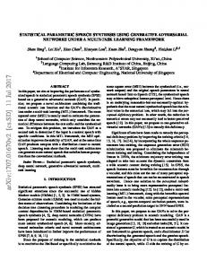
Fig. 1. Activation maps using design matrix constructed by conventional HRF model, K-SVD at p < 0.05. (a)-(c) are the activation maps using trained dictionary by K-SVD as a design matrix for three subjects, respectively. (d)-(f) are the activation maps using conventional SPM analysis for three subjects, respectively. PCA results are not illustrated since there exist no activation.

Prior to implement K-SVD, the data were spatially realigned to correct the changes in signal intensity over time which can arise from within-subject head motion. Spatial registration and normalization were applied to remove the unwanted differences to enable subsequent analysis of the data. We only extracted the voxels corresponding to the brain region from the 3-dimensional BOLD response measured with fMRI. Then the data was down-sampled at spatial direction to decrease the computation time in K-SVD learning. Since the data is a mixture of activation and noise that share some frequency band, pre-processing should be applied which removes the noise components. In fMRI, the low frequencies are known to contain unknown global trends from breathing, subject movement, vasomotion, blood pressure variation or instrumental instability which can be removed by highpass filtering. We used a discrete cosine transform (DCT) basis set with cutoff frequency of 1/128Hz to eliminate them, thus to improve the signal-to-noise ratio. After detrending, the data were temporally smoothed with time alignment using 1.5sec full-width at half maximum (FWHM) of the Gaussian smoothing kernel. We employed K-SVD algorithm to the pre-processed fMRI finger tapping data. The number of dictionary elements to train K was 50 for subject 1 and subject 2, and 53 for subject 3. Maximum coefficients to used in OMP coefficient calculations was set to 5, and 15 iterations were performed for each data. According to the algorithm, the dictionary matrix D was trained by minimizing Eq. (5). The general linear model (Worsley and Friston, 1995; Schroeter et al., 2004) is then applied to statistically analyze the measured BOLD signal. Each columns of D was entered to the design matrix d˜j shown in Eq. (8). Since they have specific pattern of neural signal, we can extract where the components come from. The ReML estimation of parameters and inference with F-statistics are then conducted using the SPM package (Wellcome Department of Cognitive Neurology, London, UK)(Friston et al., 2006).

3. METHOD 4. EXPERIMENTAL RESULTS 3.1. Behavior protocol and data acquisition The proposed method was applied to a right finger tapping (RFT) task to evaluate the performance. For the RFT tasks, the block paradigm was used. A 15 sec task period alternated with a 72 sec resting period was repeated 4 times for each subject followed by an additional 30 sec of rest. The total recording time was 480 sec. During the task period, subjects were instructed to perform a right finger flexion, and to focus on a fixed point in the resting time to minimize eye movement, thinking and so on. A total of 3 healthy right-handed subjects were examined (mean age = 25 ± 2 years). A 3.0T funtional MRI system (ISOL, Republic of Korea) was used to measure the BOLD response. During every experiments, the echo planar imaging (EPI) sequence was used with TR/TE = 3000/35 ms, flip angle = 80◦ , 35 slices, 4mm slice thickness. In the subsequent anatomical scanning session, T1-weighted structural images were acquired.

Figure 1 illustrates the resultant F-statistics maps from fMRI individual activation analysis of the right finger tapping task at p < 0.05. Figure 1(a)-(c) are the activation maps using learned dictionary by K-SVD as a design matrix entering to the sparse GLM model for three subjects, respectively. The activation maps using canonical HRF design matrix are shown below. They were determined by F-test with p < 0.05. In the case of K-SVD, the activation region was mainly localized from left primary motor cortex, decreasing noise signals rising elsewhere. It indicates the sparse dictionary learning process finds the activation signal atoms accurately, and also robust to the noise. We also implemented the PCA analysis for the same dataset to estimate the performance of the proposed method. The principal components were sorted to select the most correlated component with reference function. The selected principal component was entered to the design matrix, followed by parameter estimation and making infer-

ence with F-statistics. For three subjects, there was no activation using PCA analysis for SPM. We compared the reliability of the constructed design matrix between using K-SVD and PCA. Figure 2 shows the design matrices constructed by K-SVD and PCA. Figure 2(a),(c), and (e) are the design matrices using K-SVD for three subjects, and Figure 2(b),(d), and (f) are the design matrices using PCA, respectively. They follow the block paradigm used in our experiment well, but activation maps using them were significantly different. For all three subjects, the activation maps with p < 0.05 using trained dictionaries by K-SVD tightly localized on the left primary motor cortex, while in the case of PCA design matrix did not extract the activation region at all. In the case of subject 2, the correlation between K-SVD design matrix and canonical HRF is smaller than between PCA design matrix and canonical HRF. However, using Figure 2(c) as a design matrix works better than using Figure 2(d), as illustrated in Figure 1(b). This results indicate that the data decomposition using sparsity adapts the individual variation; and works well in the brain fMRI analysis.

(a)

(b)

(c)

(d)

(e)

(f)

5. CONCLUSION In this paper, we proposed the sparse dictionary learning for SPM, which decompose the activation signals into sparse signal atoms. This approach is based on the sparsity of neural response in fMRI measurement, so that the linear combination of decomposed dictionary constructs the robust model for the brain fMRI analysis. The data-driven design matrix containing the time course of the trained dictionary is individually adaptive. In our research, sparse dictionary learning with K-SVD extracted the activation better than conventional methods including PCA. 6. REFERENCES [1] KJ Friston, P. Jezzard, and R. Turner, “Analysis of functional MRI time-series,” Human Brain Mapping, vol. 1, no. 2, pp. 153–171, 1994. [2] KJ Friston, CD Frith, R. Turner, and RSJ Frackowiak, “Characterizing evoked hemodynamics with fMRI,” NeuroImage, vol. 2, no. 2PA, pp. 157–165, 1995.

Fig. 2. Design matrix constructed by K-SVD and PCA of the three subjects. (a),(c) and (e) are the extracted time traces using K-SVD for three subjects, respectively; (b),(d) and (f) are the time series using PCA. For all subjects, (a),(c) and (e) design matrix extracted the activation region as shown in the Figure 1, while (b),(d) and (f) failed to. The correlation values with canonical HRF are : (a)0.5740, (b)0.4167, (c)0.3369, (d)0.6717, (e)0.7011 and (f)0.5860. The red dotted lines shown in (a) and (b) are the design matrics using the canonical HRF following our experimental paradigm. [6] D. Hu, L. Yan, Y. Liu, Z. Zhou, K.J. Friston, C. Tan, and D. Wu, “Unified SPM–ICA for fMRI analysis,” Neuroimage, vol. 25, no. 3, pp. 746–755, 2005.

[3] KJ Friston, AP Holmes, JB Poline, PJ Grasby, SCR Williams, RSJ Frackowiak, and R. Turner, “Analysis of fMRI time-series revisited,” Neuroimage, vol. 2, no. 1, pp. 45–53, 1995.

[7] I. Daubechies, E. Roussos, S. Takerkart, M. Benharrosh, C. Golden, K. D’Ardenne, W. Richter, JD Cohen, and J. Haxby, “Independent component analysis for brain fMRI does not select for independence,” Proceedings of the National Academy of Sciences, vol. 106, no. 26, pp. 10415, 2009.

[4] J.C. Ye, S. Tak, K.E. Jang, J. Jung, and J. Jang, “NIRSSPM: Statistical parametric mapping for near-infrared spectroscopy,” Neuroimage, vol. 44, no. 2, pp. 428–447, 2009.

[8] KJ Friston, P. Fletcher, O. Josephs, A. Holmes, MD Rugg, and R. Turner, “Event-related fMRI: characterizing differential responses,” Neuroimage, vol. 7, no. 1, pp. 30–40, 1998.

[5] M.J. McKeown, “Detection of consistently task-related activations in fMRI data with hybrid independent component analysis,” NeuroImage, vol. 11, no. 1, pp. 24–35, 2000.

[9] M. Aharon, M. Elad, and A. Bruckstein, “K-SVD: An algorithm for designing overcomplete dictionaries for sparse representation,” IEEE Transactions on signal processing, vol. 54, no. 11, pp. 4311, 2006.