Jun 10, 2010 ... eup$Dif
STATISTICS ASSIGNMENT 1 Matteo Sostero 815831 June 10, 2010
Introduction The following document is a brief statistical report as part of the first assignment. It covers the issues raised on a dataset of 180 Veneto municipalities, particularly concerning the turnout in the European elections of 2004 and 2009. The full R code, including the commands producing tables and graphs, is given in the Sostero_Assignment_1.R file attached.1
1
Question 1
1.1
Consider the new variable Dif=V09-V04. Is there any effect of Pro on Dif?
> eup$Dif outly outly [1] -21.57 -16.75 -15.51 -15.29 -14.71 -14.48 -13.33 -13.04 -12.47 -12.17 [11] -12.09 4.80 20.86 > length(outly[outly > 0]) [1] 2 There are 13 outilers in the population of Dif of 120, only two of them are larger than 0. The two most exreme outliers are -21.57 and 20.86.
1.3
Can we assume a normal model to describe the (overall) distribution of Dif?
A fitted histogram and a quantile-quantile plot can be used to check empirically the normality of Dif. Distribution of Dif and implied normal curve
Distribution of Dif
2
●●● ● ● ● ● ● ●●● ●●● ● ●●● ●●● ● ● ● ● ● ● ● ● ● ● ● ● ● ● ● ● ● ● ● ● ● ● ● ● ● ● ● ● ● ● ● ● ● ● ● ● ● ● ● ● ● ● ● ● ●● ● ● ●● ● ● ● ● ● ● ● ● ● ● ● ● ● ● ● ● ● ● ● ● ● ● ● ● ● ● ● ● ● ● ● ● ● ● ● ● ● ● ● ● ● ● ● ● ● ● ● ● ● ● ● ● ● ● ● ● ● ● ● ● ● ● ● ● ● ● ● ● ● ● ● ● ● ● ● ● ● ● ● ● ● ●●●● ●●
0
Sample Quantiles
0.06 0.02
●
●
●
●● ●● ●●● ●●● ●●
−2
0.04
Density
0.08
4
0.10
●
● ●
●●
−4
0.00
●
−20
−10
0
10
20
●
−2
eup$Dif
−1
0
1
2
Theoretical normal quantiles
The data appear to fit vaguely the normal curve and the qq-plot. Potential causes for concern could be an imperfect symmetry of the distribution, a hint of hypernormality around the median and the presence of outliers. A more rigorous gauge of normality is given by the Kolmogorov-Smirnov test. 2
> ks.test(eup$Dif, "pnorm", mean(eup$Dif), sd(eup$Dif)) One-sample Kolmogorov-Smirnov test data: eup$Dif D = 0.1082, p-value = 0.02958 alternative hypothesis: two-sided The Kolmogorov-Smirnov test yields a p-value of 2.95%, which is low enough to question the assumption of normality of the population distribution of Dif.2 Repeating the test, but excluding outliers, suggest that they could influence heavily the result. > no_outly -12.09 & eup$Dif < 4.8] > ks.test(no_outly, "pnorm", mean(no_outly), sd(no_outly)) One-sample Kolmogorov-Smirnov test data: no_outly D = 0.0585, p-value = 0.6166 alternative hypothesis: two-sided In fact, in this case the p-value is sufficiently high to assume a normally distributed population.
1.4
Discuss the hypothesis that the population mean of Dif is equal to zero: what are the empirical findings?
A t-test can be used to check the null hypothesis H0 that µDif = 0. The alternative hypothesis is ¯ 0 : µDif 6= 0. We use a two-sided sample t-test with confidence interval 95%. H > t.test(eup$Dif, mu = 0, alternative = "two.sided", conf.level = 0.95) One Sample t-test data: eup$Dif t = -11.3749, df = 179, p-value < 2.2e-16 alternative hypothesis: true mean is not equal to 0 95 percent confidence interval: -4.486795 -3.160205 sample estimates: mean of x -3.8235 We observe that the p-value is extremely low and that the 95% confidence interval is about (-4.4, -3.1). All of which indicates that the population mean of Dif is almost surely equal to 0, with the caveat that the t-test assumes normality of the underlying population and that the Kolmogorov-Smirnov test cast doubts on this assumption.
2 2.1
Question 2 The ”male rate” Mr = 100*M/(M+F) is the percentage of males in the population of residents in a given area.
> eup$Mr ks.test(eup$Mr, "pnorm", mean(eup$Mr), sd(eup$Mr)) One-sample Kolmogorov-Smirnov test data: eup$Mr D = 0.0819, p-value = 0.1791 alternative hypothesis: two-sided The Kolmogorov-Smirnov test gives a p-value of around 17.9%, which is sufficiently high to avoid ruling out the hypothesis of normality.
2.3
Discuss the hypothesis that the population mean of Mr is equal to 50%: what are the empirical findings?
The hypothesis suggests that, in the population, males anf females are equally distributed. The null ¯ 0 : µM r 6= 50. hypothesis H0 is therefore µM r = 50, the alternative hypothesis is H We use a two-sided sample t-test with confidence interval 95% to check the hypothesis. > t.test(eup$Mr, mu = 50, alternative = "two.sided", conf.level = 0.95) One Sample t-test data: eup$Mr t = -5.3233, df = 179, p-value = 3.025e-07 alternative hypothesis: true mean is not equal to 50 95 percent confidence interval: 49.39163 49.72069 sample estimates: mean of x 49.55616 In this case, the t-test yields an extremely low p-value and a confidence interval of (49.39, 49.72), which allows us to reject the hypothesis that the population mean of Mr is equal to 50%. Furhermore, the Kolmogorov-Smirnov test reinforces the validity of this result since the underlying population appears to be normal. 4
3
Question 3
3.1
Is there any statistical relationship between Mr and Dif?
We check the relationship between the two variables by measuring their correlation: > cor(eup$Mr, eup$Dif) [1] 0.2065372 The estimated correlation coefficient is about 0.20: positive but relatively low in absolute value, which indicate weak statistical relationship and is consitent with the intuition that the relative distribution of males in any given municipality does not influence much the difference of turnout in successive elections.
3.2
Put Mf = 100*F/(M+F). Prove (theoretically) that cor(Mf,Mr)=-1 and cor(Mr,Dif)=-cor(Mf,Dif).
> eup$Mf ls_line summary(ls_line) Call: lm(formula = eup$V09 ~ eup$V04) Residuals: Min 1Q -18.5401 -2.1991
Median 0.8251
3Q 2.3953
Max 23.7348
Coefficients: Estimate Std. Error t value Pr(>|t|) (Intercept) 0.52279 3.03712 0.172 0.864 eup$V04 0.94360 0.03917 24.089 > > > > > > > > > > > > > > + >
eup$Dummy_BL