Oct 27, 2014 - of finite state Markov processes on measurement eigenvectors. .... continuous limit of a series of weak measurements where the probe is a two.
arXiv:1410.7231v1 [math-ph] 27 Oct 2014
Statistics of quantum jumps and spikes, and limits of diffusive weak measurements Michel Bauer1 , Denis Bernard2 , and Antoine Tilloy2 1
2
Institut de Physique Th´eorique, CEA Saclay & CNRS, Gif-sur-Yvette, France Laboratoire de Physique Th´eorique de l’ENS, CNRS & Ecole Normale Sup´erieure de Paris, France
Abstract This paper is devoted to the quantitative study of quantum trajectories of systems subjected to a tight and continuous monitoring. These trajectories exhibit quantum jumps, observed in various experiments, but also more surprising features, quantum spikes, revealed in this study. We give a quantitative understanding of quantum jumps and spikes, starting from the stochastic differential equation obeyed by the density matrix of a quantum system undergoing continuous measurement. We show that jumpy evolutions between pointer states emerge in the strong measurement limit: the system finite dimensional distributions behave as those of finite state Markov processes on measurement eigenvectors. We compute the corresponding jump rates analytically. Beyond the convergence of finite dimensional distributions, we show the ubiquitous emergence of quantum spikes, which we conjecture to have universal scale invariant fluctuations described by Poisson point processes. This result is proved in two cases: general two-level systems and systems whose evolution preserves the diagonality of the density matrix. We argue that quantum spikes give a very clear and general signature of measurement induced quantum jumps, a feature which could be of experimental interest. We eventually apply our general results to several examples: we recover well known facts about the quantum Zeno effect and more surprising results on thermal fluctuations and on control.
1
Contents 1 Introduction
2
2 Main Results
4
3 Applications 3.1 Simple Hamiltonian . . . 3.2 Simple thermal jumps . . 3.3 The general diagonal case 3.4 Tilted thermal jumps . . . 3.5 Double Quantum Dot . .
. . . . .
. . . . .
. . . . .
. . . . .
. . . . .
. . . . .
. . . . .
. . . . .
. . . . .
. . . . .
. . . . .
. . . . .
. . . . .
. . . . .
. . . . .
. . . . .
. . . . .
. . . . .
. . . . .
. . . . .
. . . . .
. . . . .
10 10 10 12 12 14
4 Details on the finite state Markov process limit 17 4.1 Proof of Proposition 1 . . . . . . . . . . . . . . . . . . . . . . . . 17 4.2 What is the most general jumpy scaling limit? . . . . . . . . . . 21 5 Details on the spike statistics 22 5.1 Proof of Proposition 2 in two level thermal case . . . . . . . . . . 22 5.2 The general diagonal case . . . . . . . . . . . . . . . . . . . . . . 25 5.3 Proof of Conjecture 1 in the two level pure hamiltonian case . . . 29 6 Details on peculiar Markov processes
1
32
Introduction
Recent advances in experimental techniques now allow for a tight monitoring of small open quantum systems. A striking feature of such systems undergoing continuous measurement is the emergence of a jumpy behavior between measurement pointer states. This interesting and ubiquitous phenomenon has already been observed in many experiments [19, 10, 22]. Even if quantum jumps were already well known to Bohr [11] and even if recent progress have been made, notably to show that they were detector dependent [25], to our knowledge, their statistics have never been studied thoroughly and neither have the surprising details of the spike statistics. This investigation is the main purpose of this article. We conduct our study using the formalism of continuous measurement developed in [2, 13, 3, 24, 9, 4], that is we study a stochastic differential equation (SDE) with Gaussian noise describing the (continuous) evolution of the density matrix of a small open system of interest. The stochasticity comes from the conditioning of the density matrix on the (random) measurement outcomes. Such equations can be obtained as the limit of a series of weak measurements carried out on a quantum system[1, 20, 21]. In this setting, the jumpy regime arises when the rate of measurements, that we call γ 2 , is large. At this point we should emphasize that these quantum jumps obtained in the large γ limit
2
of continuous equations are not the same as those emerging from the intrinsically discontinuous Poissonian unraveling of a quantum master equation. This otherness is underpinned by a clear and peculiar signature of these jumps : the survival of quantum spikes, that are scale invariant fluctuations of the density matrix corresponding to aborted jumps. These spikes do not disappear in the scaling limit and their statistics are tied to the jump rates. From a mathematical perspective, we study a class of non-linear SDE in the strong noise limit, and show that the solution converges, in a very weak sense, to a continuous-time finite-state Markov process on the measurement pointer states and we compute the transition rates. In precise mathematical terms, we show that the finite dimensional distributions converge weakly (i.e. in law) towards those of a finite-state Markov process on the measurement pointer states. But the process itself, which is continuous at finite γ, does not converge weakly in any space of cadlag (right continuous with left limits) functions1 . The emergence of jumps and the computation of the rates are actually surprisingly cleaner to prove in this setting that in the usual Kramers limit of small noise. Eventually we believe this study provides a quantitative understanding on the semi-classical behavior of tightly monitored quantum systems and as such it could have applications to a wide class of microscopic open systems showing a jumpy behavior (quantum dots, photons in cavity,...). Outline This paper is structured as follows. We first present our main results in section 2 and relegate the proofs to section 4 for the rate computation and section 5 for the derivation of the spike statistics. As our results are very general we show in section 3 how they apply to four examples: – A 2-level system evolving unitarily. We compute the jump rates and recover the quantum Zeno effect in a quantitative manner. – A 2-level system coupled to a thermal bath. We obtain a jumpy behavior at a rate proportional to the coupling to the bath and occupation probabilities consistent with the Gibbs distribution. We subsequently generalize this study to a N -level system. – A 2-level system coupled to a thermal bath with a measurement eigen-basis tilted from the energy basis. We obtain jump rates proportional to the coupling to the bath but peculiar occupation probabilities. We discuss briefly the physicality of this setup. – A 3-level system with a unitary dynamic and a coupling to a bath. This paradigmatic example inspired from a double quantum dot shows transitions that can be Zeno frozen (as in the first example) and jumps with rates independent from the measurement rate (as in the second and third examples). We use this complex behavior to control the system using only the measurement rate. We obtain an original quantum Maxwell Daemon as a natural byproduct. In the last section, we eventually provide more mathematical details on the peculiar Markov processes that appear throughout our paper. 1 Thus convergence is weak also in the sense that some interesting quantum fluctuations, spikes, are preserved in the limit.
3
2
Main Results
We consider a very general quantum system, but with a finite dimensional Hilbert space, whose dynamics are prescribed by a Liouvillian L. We assume that an observable O is also continuously measured at a rate, or strength, γ 2 (say through homodyne detection in quantum optics for example) with efficiency η (taken to be 1 when not explicitly mentioned later). As a result the density matrix of the system evolves in the following way [26]: √ dρt = L(ρt ) dt + γ 2 LN (ρt ) dt + γ η DN (ρt ) dWt ,
(1)
where Wt is a standard Wiener process, and N is the so-called measurement operators with O = N +N † the measured observable, LN (ρ) = N ρN † − 21 {N † N, ρ} is the Lindblad generator associated to N and DN (ρ) = N ρ + ρN † − ρ tr(Oρ) the stochastic innovation term 2 . Any given realization of the Wiener process corresponds to a sample of time series of measurements. Measurement outputs xt are random according to the rules of Quantum Mechanics and given √ by dxt = tr(Oρ) dt + η dWt [26]. Solutions of eq.(1) are called quantum trajectories. We will write everything in the basis where O is diagonal, i.e. P O = k λk |kihk| and suppose that all its eigenvalues are different. P We assume that the measurement operators N are diagonal in this basis, N = k νk |kihk| with λk = νk + ν¯k = 2 Re νk , in order to ensure for the process to be a nondemolition measurement in absence of the dynamics generated by the Liouvillian L. The eigenstates |ki will be called pointer states in what follows. Remark. The diffusive measurement scheme we consider can be seen as the continuous limit of a series of weak measurements where the probe is a two level object in a pure state which interacts weakly with the system before being projectively measured [1, 20, 21, 5]. The operator N is then a function of the microscopic details of the interaction and η codes for the fraction of probes that are effectively measured. The generalization to probes in a mixed-state (say a thermal state for example), and/or to probes with more than two levels, is straightforward and our formula can be extended easily in this framework. However such an extension makes the notations even messier and we choose to trade a bit of generality for a slightly clearer presentation. When γ is large, the system density matrix will undergo quantum jumps between the pointer states of the observable O. Our objective is to characterize those jumps at the stochastic process level and not only at the ensemble average level, i.e. we want to show that the conditioned density matrix is itself, as far as the diagonal is concerned, a finite state Markov process in the large γ limit and not only that the diagonal of the unconditioned density matrix is the probability density associated to a finite state Markov process as in [17, 14]. 2 Notice that we use the same notation as in [23] for consistency but that the latter differs from Milburn and Wiseman’s [26]. The dictionary is the following: LN (ρ) = D[N ]ρ and DN (ρ) = H[N ]ρ. We prefer to use the letter L for the Lindbladian and to reserve the letter H for an Hamiltonian, and we use the letter D for the term multiplying the Brownian noise as a reference to a non-linear diffusion coefficient.
4
Especially, the first objective of this paper is to show how the jump rates between different states depend on the parameters of the Liouvillian L and as a result how they also characterize it. Inbetween jumps the density matrix fluctuates and is subject to large deviations on a very short time scale (actually on a time scale going to 0 at large γ) which correspond to unsuccessful attempts to jump. We call them quantum spikes. The second objective of this paper is to give a concise description of the statistics of these fluctuating spikes in the large γ limit. The way to proceed will be to code their extrema in Poisson point processes and to give a procedure to reconstruct the density matrix fluctuations from samples of these processes. We first need to say a brief word about the scaling limit in order to state the results, and it will be more carefully explained later in the text. It is well known that if L is generated by a simple Hamiltonian, a continuous strong measurement will tend to Zeno freeze the system in one of the pointer states for an arbitrary long time, i.e. when γ → ∞ all the jump rates will go to 0. As a result and to get meaningful predictions in this limit, we need to adequately rescale the different parts of the dynamics to keep finite jump rates in the large γ limit. Such a rescaling is not required for all parts of the dynamics because as was argued in [6], jumps that emerge from a dissipative coupling cannot be Zeno frozen. To get the most general scaling limit we consequently need to split the Liouvillian into different parts, actually four, that need to be rescaled separately. We write Qi for the diagonal coefficients of ρ in the measurement eigenbasis, the probabilities, and Uij for the non diagonal coefficients of ρ, the (not yet rescaled) phases, Qi := hi|ρ|ii,
Uij := hi|ρ|ji, i 6= j.
We decompose L in four super-operators, A that sends the probabilities to the probabilities, B the phases to the probabilities, C the probabilities to the phases and D the phases to the phases. � ∂t Qi = A(Q)i + B(U)i (=: Aki Qk + Bikl Ukl ) ∂t ρt = L(ρt ) ⇐⇒ k kl ∂t Uij = C(Q)ij + D(U)ij (=: Cij Qk + Dij Ukl ) notation Summation over repeated indices is implicit. The reason why this decomposition is legitimate will be clearer later but a good rationale for it is that as the strong measurement will tend to shrink the phases, they will obviously need a differentiated treatment from the probabilities. We now claim that A needs no rescaling, that C and B need to scale like γ and D like γ 2 . In what follow, we thus write : A = A, B = γB, C = γC, D = γ 2 D. (2) For such a scaling to be consistent with the complete positivity of the map generated by L in the large γ limit, we will see that D needs to be diagonal: kl Dij = −dij δik δjl
We should also add that equation (2) only gives the dominant terms in an expansion in power of γ and that the sub-leading corrections may in general be 5
needed for compatibility with the complete positivity of the map associated to L. We just claim that they have no impact on the large γ limit as expected and omit them for clarity. Our first main result, which will be proved in section 4.1, can then be stated as follows: Proposition 1. With the previous notations, when γ → ∞ the finite dimensional distributions of the conditioned density matrix ρt converge to those of a finite state Markov process on the projectors associated to the measurement eigenvectors. The jump rate from site i to site j then reads in terms of the rescaled coefficients: i X Ckl Bjkl (3) mij = Aij + 2 Re ∆kl k 0,
i ykl (t) := E[Ykl |Q· = δ·i ] −→
t→+∞
19
i Ckl . ∆kl
Recall that ∆kl := 12 (|νk |2 + |νl |2 − 2νk ν¯l )2 + dkl . R We can now compute the transition rates mij = dµi (D0 fj ). The operator D0 can be easily computed as it is the operator associated to the (S)DE dQi = A(Q)i dt+B(Y)i dt, without noisy terms, so that D0 is the first order differential operator: X D0 = [A(Q)i + B(Y)i ] ∂Qi (27) i
Recalling that fj (ρ) = Qj we get (with implicit summation on repeated indices): Z Z i i mj = dµ (D0 fj ) = δ i (Q) dµiY [Akj Qk + Bjkl Ykl ] Z Z = Akj δ i (Q)Qk + Bjkl dµiY Ykl (28) = Aij +
i X Bjkl Ckl kl
∆kl
,
which is the result that was announced previously. Remark. In particular, because the fi ’s are dual to the dµj ’s and equal to Qi , at large γ we simply have Z X X �j �j E[Qi (t)] = fj (ρ0 ) etM k dµk Qi = Qj (0) etM i , j
jk
P or equivalently, ∂t E[Qi (t)] = j E[Qj (t)] mji . Notice however that the above description of the limiting kernel is finer than this finite state Markov process formula. Remark. For completeness we give here an implicit expression of the measure dµiY via an explicit expression of the large time limit of Ykl conditioned on Ql → δil . Under that condition, the Ykl ’s satisfy the decoupled SDEs � � � � √ i dYkl = Ckl − ∆kl Ykl dt + η Ykl νk + ν¯l − λi dWt , whose solutions are i Ykl = Ckl
Z
t
1
i2
i
ds e−(∆kl + 2 βkl )(t−s)+βkl (Wt −Ws ) .
√ i with βkl := η(νk + ν¯l − λi ). Recall that Wt − Ws ≡ Wt−s in law. At large time, these solutions converge in law to Z ∞ i i2 t i Ykl∞;i := Ckl ds e−∆kl t e+βkl Wt −βkl 2 , 0
whose distribution is the measure dµiY by construction. In the above expresi i2 t sion, we recognize the standard exponential martingale e+βkl Wt −βkl 2 . Hence, R ∞ ∞;i i i E[Ykl ] = Ckl ds e−∆kl t = Ckl /∆kl as we found previously. 0 20
In the special case when the equation for Ykl is real, the equation for the stationary measure dµiY turns into an ordinary differential equation which can be solved explicitly : for the equation dYt = (C − ∆Yt )dt + βYt dWt , with C, ∆, β real, one finds for the stationary measure an inverse Γ-distribution 1 dµ(y) = Γ(1 +
dy − β2C e 2y 2∆ y ) 2 β
�
2C β2y
�1+ 2∆2 β
,
which clearly has a heavy tail and a finite number of moments. The explicit distribution in the complex case is not known.
4.2
What is the most general jumpy scaling limit?
We now prove that we have derived the most general scaling limit that gives rise to quantum jumps. For A, B and C we obviously have the most general scaling as if they were scaled with a smaller power, they would become irrelevant in the scaling limit (or equivalently the Zeno effect would kill the associated transition rates), and if they were scaled with a bigger power, the jump rates would diverge in the large γ limit and the limit would not be jumpy anymore. To say it differently, the simple fact that we ask the limit to be jumpy and that the system parameters have an influence fixes completely the scaling. We now need to show as we previously announced that the phase-phase coupling term D in the Liouvillian is always irrelevant no matter how it is rescaled unless it is diagonal. We will first show that that the non diagonal terms cannot grow faster than γ and then prove that such a limiting scaling would still make them irrelevant. D cannot grow faster than γ, unless diagonal: Let us suppose that D can grow faster than γ. It would then need to be rescaled independently of A, B and C which were shown to grow no faster than γ. As a result D needs to be itself the generator of a completely positive map Φt that couples only the phases with the phases. Let us suppose that we have a completely positive application Φt with generator L˜ that couples only the phases and write it using the usual decomposition: � � � X� a 1 ˜ M ρM a † − {M a † M a , ρ} , L(ρ) = −i H, ρ + 2 a for some operators M a . We ask that L˜ does not act on the diagonal coefficients, ˜ i.e. L(|iihi|) = 0 for any projector on the measurement eigenvector |iihi|. In ˜ particular, imposing that the diagonal elements vanish, i.e. hj|L(|iihi|)|ji =0 for any j, reads � X � a 2 Mji − δij (M a † M a )jj = 0. a
Thus, for j 6= i, we get X a 2 Mji = 0, a
21
(29)
a and hence Mji = 0 for all a and j 6= i. That is, all the M a ’s are diagonal matrices. The Hamiltonian part of the flow also needs to be diagonal. Indeed, if Hkl 6= 0 for some k and l, k 6= l, we have hk|[H, |lihl|]|li = Hkl so H couples the probabilities to the phase which is forbidden. Therefore, P aH is also diagonal and a as a result L˜ cannot mix the phases. Writing M = k nk |kihk|, this means that P ¯ aj ) + i(Hii − at most D(Y)ij = −Dij Yij , with Dij = 12 a (|nai |2 + |naj |2 − 2nai n Hjj ), a term that is proportional to the deterministic part of the measurement acting on the phase. The only non-trivial consistent scaling is that D scales as γ 2 and D(Y )ij = −γ 2 dij Yij . If D scales as γ then it is irrelevant: Let us suppose that D = γD which is the limiting scaling allowed for a non-diagonal D. In that case the FokkerPlanck operator associated to equation (1) needs to be written with a new term of order γ that is D = D0 +γD1 +γ 2 D2 where D1 is the Fokker-Planck operator P kl kl associated to the (S)DE: dYij = Dij Ykl dt. We thus have D1 = ijkl Dij Ykl ∂Yij . We now proceed with the same perturbative expansion as before except this 2 time we assume that a term of order γ remains, i.e. that Kt = etγ D2 +tγD1 +tD0 . The first two terms of the eigenvalue expansion will need to be zero to give a non trivial jumpy behavior in the large γ limit. We use the same notation as before, that is:
FI = fI + γ −1 fI1 + γ −2 fI2 + ... EI = 0 × γ 2 + 0 × γ + e0I + ...
(30)
for the eigen-modes with leading vanishing eigenvalues. We then have, up to second order in γ: D2 fI = 0 D2 fI1 + D1 fI = 0 D2 fI2
+
D1 fI1
(31)
+ D 0 fI = e I fI
Recall that the f ’s only depend on D2 and are thus the same as before, that is fi (Q, Y) = Qi which gives in particular D1 fI = 0. In that case we have D2 fI1 = 0 so that fI1 ∈ Ker(D2 ) and as a consequence, D1 fI1 is also zero. As a result, the terms of order γ no longer have any role to play in the computations and D is irrelevant.
5 5.1
Details on the spike statistics Proof of Proposition 2 in two level thermal case
Here we prove that, in the case of a two level system coupled to a thermal bath under continuous monitoring of its energy, the limiting jump process, including all spikes, may be reconstructed from the Poisson point process defined in Proposition 2 of section 2. Recall that in this case we can restrict the analysis to the diagonal elements of the density matrix. Let Q := h0|ρ|0i and h1|ρ|1i = 1−Q
22
with |0i and |1i the two energy eigenstates of this system. Under continuous monitoring of the energy with efficiency η, it satisfies the SDE dQ = α(p − Q) dt + γ
√
η Q(1 − Q) dWt .
(32)
That is: A00 = −α(1−p), A10 = αp in the notation of section 3.2. Here p = 1/(1+ e−βω ) for a thermal bath at temperature 1/kB β with ω the energy difference between the states |0i and |1i. For convenience, we set λ0 − λ1 = 1 with λk the eigenvalues of the observable O. The quantum trajectories take place on the interval [0, 1], spending most of their time at the vertices Q = 0 and Q = 1 (recall Fig. 3). In this simple case, Proposition 2 claims that the quantum trajectories can be reconstructed from two Poisson point processes valued on [0, 1] × R+ with respective intensities, h dQ i dν0 = αp dt · δ(1 − Q)dQ + Q2 , (33) h dQ i dν1 = α(1 − p) dt · δ(Q)dQ + . (1 − Q)2 The first measure is associated to the spikes and jumps starting from vertex Q = 0, the second to those starting from Q = 1. The reconstruction of the quantum trajectories from samples of these point processes has been explained in Example 2. Let us assume for a moment that the maximum heights of the spikes of the trajectories form a Poisson point process. To prove that the reconstruction procedure reproduces quantum trajectories with the correct statistics we only have to verify that the intensity of the point process is the correct one. We shall do it by checking two statements which have been proved [6] to hold true for quantum trajectories by a direct analysis of the above SDE (32) in the large γ limit. The first is related to the distribution of the time interval between two jumps and the second to the distribution of the maximum height of the spikes. Namely: i) The time duration between two successive jumps is a Poisson variable with mean 1/αp for jumps from Qi → 0 to Qf → 1, and 1/α(1 − p) for jumps from Q = 1 to Q = 0; ii) For 0 < Qi < ε < Q < 1, the probability for a quantum trajectory starting at ε to reach the height Q before going back to Qi → 0 is ε/Q. The last statement is a claim about the distribution of the maximum height of the spikes starting from 0 conditioned to be bigger than ε. These statements were proved in [6] directly from eq.(33). The proofs in [6] involve a limit γ → ∞ at fixed Qi , ε and Q. We are then extending these results by then taking the limit Qi → 0. Recall that a Poisson point process on measurable space M with intensity ν is characterised by the following properties: (i) For any measurable set U ⊂ M, the number NU of points in U is a Poisson variable with mean ν(U ); (ii) For any
23
family U1 , U2 , · · · , Un of disjoint measurable sets in M, the random numbers NU1 , NU2 , · · · , NUn are independent random variables. The first point i) is easy to prove. Suppose that the trajectory is at Q = 0 at time t = 0. The probability that the first jump occurs at time t, up to dt, is the probability that the sample of the process associated to the vertex Q = 0 contains no point in {1} × [0, t] and a point in {1} × [t, t + dt] with dt vanishingly small. This probability is: h i P N{1}×[0,t] = 0, N{1}×[t,t+dt] = 1 = e−ν0 ({1}×[0,t]) · ν0 ({1} × [t, t + dt])e−ν0 ({1}×[t,t+dt]) = e−αpt αp dt. To prove the second point ii) consider a sample for which a spike started at zero goes above ε and compute the probability that that this spike goes further above Q. This is the probability that, conditioned on having a point on {[ε, 1]×[0, δt]} with δt vanishingly small, the sample of the process associated to the vertex Q = 0 contains no point in [ε, Q]×[0, δt] and one point in [Q, 1]×[0, δt]. That is: h i P N[ε,Q]×[0,δt] = 0, N[Q,1]×[0,δt] = 1 N[ε,1]×[0,δt] = 1 =
ν0 ([Q, 1] × [0, δt]) ε = ν0 ([ε, 1] × [0, δt]) Q
Notice that these two computations completely fix the intensity of the point process, including the δ(1 − Q)dQ and dQ/Q2 terms. The fact that the spike process is indeed a Poisson process is made very likely by property i) and one proves it by using a third property established in [6]: iii) For 0 < ε < Q < 1, the limit for γ → ∞ of the distribution of the first ε instance that a trajectory starting at ε reaches the point Q is Q δ(t)dt + (1 − ε αp − Q) Q e
αp Q t
dt. This result is appropriate to deal with the maxima, and there is a twin formula for the minima. We shall use freely that, seen as a function of time, the maximum heights of the spikes of the trajectories form a process which is Markov as a limit of Markov processes. The meaning of iii) is the following: in the large γ limit, starting from ε, either reaching Q take no time ε ε (with probability Q ) or (with probability 1 − Q ) it takes an exponential time αp with parameter Q . Note that this parameter does not depend on ε. Thus, either Q is reached immediately, or 0 is reached immediately, and from there it takes an exponential time with parameter αp Q to reach Q. Together with ii), iii) (of which i) is a simple consequence) implies immediately that, starting at 0, it takes an exponential time with parameter αp ε to reach ε (note that this is consistent with i) for ε → 1) and then the actual maximum Q ≤ 1 reached before falling back to 0 is distributed as P (Q ≥ q) = ε/q. Thus, by the Markov property, the point process of maxima above ε is just a Poisson 24
point process with intensity
αp ε
h dt · ε δ(1 − Q)dQ +
dQ Q2
i , which is exactly dν0
restricted to [ε, 1]×R+ . By taking ε → 0 one recovers the announced result. Conversely, we can derive formula iii) starting from the Poisson description. One needs to compute the distribution of the first time the trajectory reaches Q starting at ε. Conditioning to start at ε amounts to condition the point process to have a point in [ε, 1] × [0, δt] with δt vanishingly small. We aim at computing the distribution of the occurrence time for the first spike going further above Q happening after this spike above ε. There are two possibilities. The first one is realized when the initial spike above ε is actually above Q, so that the occurrence time is zero. This happens with probability i ν ([Q, 1] × [0, δt]) h ε 0 = . P N[Q,1]×[0,δt] = 1 N[ε,1]×[0,δt] = 1 = ν0 ([ε, 1] × [0, δt]) Q The second one is realized when the spike above Q is different than the first spike above ε. The probability that its occurrence time is t, up to dt, is then h i P N[ε,Q]×[0,δt] = 1, N[Q,1]×[0,t] = 0, N[Q,1]×[t,t+dt] = 1 N[ε,1]×[0,δt] = 1 ν0 ([ε, Q] × [0, δt]) ν0 ([Q, 1] × [t, t + dt]) −ν0 ([Q,1]×[0,t]) e ν0 ([ε, 1] × [0, δt]) � � αp ε αp dt. = e− Q t 1 − Q Q
=
Summing up the two above contributions gives the correct distribution for this stopping time. Computations for jumps and spikes starting from Q = 1 are done similarly.
5.2
The general diagonal case
Strategy of the proof. The proof of proposition 2 in the general case is a bit long and technical but it is nevertheless interesting. We recall here the strategy of the demonstration that was outlined just after Example 2. The core of the proof consists in proving a technical lemma stating that the quantum trajectories of the diagonal density matrix localize along the edges of S. This result will bring the general case back (locally) to the study of decoupled 2-level systems, a case that was treated in the previous section. The rest of the proof will be straightforward. We first start by making a few general remarks about the trajectories we consider. Though not strictly necessary for the proof, we hope they will give a heuristic understanding of the jump process and of the spikes. Preliminary remarks. We would first like to develop a slightly more precise picture of the trajectories in the strong measurement limit. We know that at large γ the system Pspends most of its time close to the corners of the probability simplex Qi ≥ 0, i Qi = 1. The typical distance to corner i when the system is
25
close to Qi = 1 is5 ∼ Aii /γ −2 . The fact that trajectories remain close to corners most of the time is entirely due to the measurement process, which for large γ dominates system-environment interactions. Measurement (the dWt contribution) leads the system to converge to a corner, and is effectively compensated by system-environment interactions (the dt term) when the distance to a corner becomes of order ∼ Aii /γ −2 as mentioned above. But from time to time a jump occur almost instantaneously: at finite but large γ the time scale is typically ∝ γ −2 (if η is of order 1). Our aim is to describe some qualitative features of the trajectory during such jumps, and for that we shall have to zoom the time scale. We shall explain why they take place along edges, which even reinforces our result of convergence towards a finite state Markov process: at large γ, trajectories occupy only a small neighborhood of the graph associated to the Markov process (remember that the graph made of the vertices and edges of a simplex is the complete graph), the 2, 3, · · · -faces of the simplex play no significant role. The stochastic differential equation for the diagonal part of ρ contains two pieces : a measurement part, involving dWt , and a system-environment interaction part, involving dt. This part tends to lead the system to (one of) the equilibrium distribution(s), so generically it tends to take the Qi ’s away from the boundary of the simplex.Thus, just as measurement is responsible for the tendency of trajectories to spend most of their time close to vertices, if there is a tendency to remain close to edges during jumps, it has to be due to measurement as well. What we shall show is that under measurement, a trajectory starting close to a corner and conditioned to end in another one does the transition by remaining close to the corresponding edge. Before giving the argument, we make the following remark. To fix notation, we assume that the labels of the two distinguished vertices are 0 and ∞. If a point started at vertex 0 (i.e. Qi = δi0 ) is left for a small time ∆t under the sole influence of system-environment interactions, it ends at Qi ∼ δi0 + A0i ∆t. If then system-environment interactions are turned off and only measurement is considered, the Martingale convergence theorem (which in that case justifies and reproduces the standard rules of measurement in quantum mechanics) says that the trajectory will end at vertex i with probability Qi , so that if conditioned to make a jump, i.e. to end at a vertex different from 0, it will end at vertex ∞ with probability −A0∞ /A00 , just as predicted by jumping rates for the finite state Markov process described by A. Conditioning on transitions from vertex I0 to vertex I∞ . The equation for measurement is X dQi = Qi (λi − Qk λk )dWt , k
where we have removed the measurement strength factor because we want to 5 This can be inferred at least heuristically by looking back at the simplest case, with only two states: A good approximation close to the corner is dQt = λ(p − Qt ) + γQt (1 − Qt )dWt . It is straightforward to compute the invariant measure and the location of the two probability peaks when λ/γ 2 → 0+ [6].
26
focus on the jump. Let P denote the original measure (under which Wt is a Brownian motion), and let P be the measure when conditioned to end at Qi = δi∞ . The first thing to compute is the new equation under P. The conditioning martingale is Q∞ (t) and Girsanov’s theorem implies that W t = Rt P Wt − 0 dsQ∞ (s)(λ∞ − k Qk (s)λk ) is a P Brownian motion. As the Qi (t)’s are P martingales, the Ri (t) := Qi (t)/Q∞ (t) are P martingales, and an application of Itˆ o’s formula gives dRi (t) = (λi − λ∞ )Ri (t)dW t , which integrates to 2
Ri (t) = Ri (0)eλi W t −λi t/2 where we have set λi := λi − λ∞ . The λi , i 6= ∞ are all nonzero, so that the corresponding Ri (t) converge towards 0 with probability 1 (as they are martingales with expectation Ri (0) 6= 0 in general, this P is a case when convergence cannot take place in L1 ). Using the normalization i Qi = 1 we find: 2
Ri (0)eλi W t −λi t/2 . Qi (t) := P 2 λj W t −λj t/2 R (0)e j j Some Brownian probabilities. In the following arguments, we shall use freely the following facts for Brownian motion with a constant drift. Let Xt = ±W t + νt where ν > 0. Then one can prove the following: 1) Let x < 0 then P [Xt > x, ∀t ≥ 0] = 1 − e2νx 2) Let x > 0. Then Z
t
P [∃s ≤ t, Xs > x] = 0
ds x − (x−νs)2 2s e . (2π)1/2 s3/2
We shall only need the fact that for x, t → +∞ with
x−νt √ t
→ +∞ the rough
(x−νt)2 − 2t
order of magnitude of the right-hand side is e . 3) Let x be arbitrary. Then Z +∞ � � (y−νt)2 dy P [Xs > x, ∀s ≥ t] = e− 2t 1 − e2ν(x−y) . 1/2 (2πt) x We shall only need the fact that for x, t → +∞ with
x−νt √ t
→ −∞ the right-hand
(x−νt)2 − 2t
is close to 1 with corrections roughly of order e . Armed with the first formula, the third is elementary: under the integral sign, the first factor is the density of Xt and the second is the probability, when sitting at y at time t, to never come back to x. Proof of the main lemma From now on we concentrate on one of the states, call it 1 6= 0, ∞. We set r := R1 (0) and R := R0 (0). We now have everything needed to state and prove the following technical lemma: 27
Lemma 2. There is a κ > 0 such that for R := R0 (0) large enough: � � −κ P sup Q1 (t) ≤ R > 1 − R−κ .
(34)
t
In fact we shall show a bit more : one could trade a better exponent for the bound on Q1 (t) at the price of a worse exponent for the probability. Proof. There is one special case that can be dealt with easily : suppose that 2 2 λ1 > λ0 . From the formula for Q1 (t) we infer that 2
Q1 (t) ≤
reλ1 W t −λ1 t/2 2
Reλ0 W t −λ0 t/2
=
r −|λ1 −λ0 |(±W t +|λ1 +λ0 |t/2) e . R
Thus � � � � r P sup Q1 (t) ≤ δ ≥ P sup e|λ1 −λ0 |(±W t −|λ1 +λ0 |t/2) ≤ δ , t t R and by fact 1) the right-hand side is 1−
� r � λ1 +λ0 λ1 −λ0 . δR
Thus we see that the estimate (34) holds whenever κ
0. Thus from the inequality ( ) 2 2 reλ1 W t −λ1 t/2 , reλ1 W t −λ1 t/2 , Q1 (t) ≤ min 2 Reλ0 W t −λ0 t/2 one should be able to infer a quantitative version of the statement that Q1 (t) remains small at all times. We observe that, for an arbitrary time τ we have ( ) 2 2 reλ1 W t −λ1 t/2 λ1 W t −λ1 t/2 sup Q1 (t) ≤ sup sup , sup re . 2 t t≤τ Reλ0 W t −λ0 t/2 t≥τ The idea is to use property 2) for the first bound and property 3) for the second bound, and then optimize τ . Recall that measurement is assumed to be nondegenerate, so that λ1 6= λ0 . λ1 W t −λ2 t/2 |λ0 +λ1 | The condition that re λ W t −λ12 t/2 ≤ δ can be rewritten as ±W t + t≤ 2 Re
1 |λ0 −λ1 |
log
δR r .
0
0
2
The condition that reλ1 W t −λ1 t/2 ≤ δ can be rewritten as ±W t + 28
|λ1 | 2
t≥
1
|λ1 |
log rδ . Setting x0 :=
1
|λ0 −λ1 |
log
δR r ,
ν0 :=
|λ0 +λ1 | 2
, x∞ :=
1
|λ1 |
log
r δ
|λ1 |
x0 √ −ν0 τ are all large and 2 , we recognize that if τ , x0 , x∞ and τ x∞√ −ν∞ τ while is large and negative, 2) and 3) imply that P(supt Q1 (t) ≤ τ
and ν∞ :=
positive δ) will 1 by a small � differ from � quantity which will be of rough order ∆ := (x −ν τ )2 (x −ν τ )2 − 0 2τ0 − ∞ 2τ∞ max e ,e . We can use τ to optimize. This amounts to equate the two exponents, −x∞ ν0 +x∞ , leading to x0 − ν0 τ = −(x∞ − ν∞ τ ) = x0 νν∞ . i.e. to set τ = xν00 +ν ∞ 0 +ν∞ 2
(x0 ν∞ −x∞ ν0 ) Thus log ∆ = − 2(x . If one inserts that δ := R−κb , one finds that 0 +x∞ )(ν0 +ν∞ ) log ∆ = −κp log R + subdominant terms. The condition that x0 − ν0 τ should be large and positive implies that κb < (λ1 /λ0 )2 < 1. The exponent κp is a quadratic polynomial in κb . Our bound for κ is obtained by taking κb = κp . When κ is strictly less than this value, relation (34) holds. The algebra leading to the value of our bound for κ is straightforward but cumbersome, and the bound is not illuminating. As we do not expect it to be accurate (it is probably way too small), we simply quote a special case: if λ0 = −2λ1 , then (34) holds √ for for κ < 26−5 ∼ 1/40, a rather small number indeed. 4 Anyway, for each face ijk of the simplex where ij is an oriented edge and k a direction to move away from it, there is an exponent κi,j,k for which (34) holds. We can define κ as the smallest of among all of them, which ends the proof of the lemma.
Conclusion of the proof. We can finally return to our original motivation. We know that away from the boundary of the simplex, i.e. outside a simplicial shell of typical thickness 1/γ 2 , the trajectories are governed by measurement. The computations above show that in fact they remain close to the edges, in a skeleton shell of thickness bounded by γ −2κ with probability larger than 1 − γ −2κ . Thus in the limit γ → ∞, the jumps take place along the edges, really mimicking the behavior of a standard finite state Markov process for which only the skeleton graph makes sense, and not the simplex. Now restricting the evolution along one of the edges emerging from vertex I0 , say from I0 to I∞ , only Q0 and Q∞ are non zero and sum to one. Their evolution equation are those of a thermal two level system parameterised by 0 two couplings A∞ 0 and A∞ and the maxima of Q∞ are governed by the Poisson process associated to the two level system.
5.3
Proof of Conjecture 1 in the two level pure hamiltonian case
We look at the case of two level system evolving unitarily but under continuous monitoring (of an observable not commuting with the Hamiltonian). For simplicity we take H proportional to σy , i.e. H = (ω0 /2)σy so that the density matrix coefficients are real numbers. We take N = γσz /2, that is O = γσz (and η = 1). In such a situation, it has been shown that the system purifies so that 29
we can restrict our study to pure states (see [18] for a general proof and [7] for an ad-hoc proof in this setting). Restricting to pure states, the density matrix can be parameterised by an angle θ such that ρ11 = Q = 12 (1 + cos θ) and ρ12 = U = 12 sin θ. With this change of variable, the system density matrix evolution reduces to: dθt = −(u γ +
γ2 sin θt cos θt ) dt + γ sin θt dWt . 2
(35)
As described in [7] one has to be careful and look separately at the process in the upper semi circle, i.e. θ ∈ [0, π] modulo 2π, and in the lower circle, θ ∈ [−π, 0] modulo 2π. For u > 0, the process always enters [0, π] from π and leaves it from 0 (and symmetrically for the other interval). For γ large, the fixed points are at π − ∈ [0, π] corresponding to Q = 0 and at 0− ∈ [−π, 0] corresponding to Q = 1. We shall look at the process for θ ∈ [0, π] so that we are going to describe the jumps and spikes started at Q = 0. The process defined by eq.(35) can be studied using standard probability tools. Because it is a one dimensional SDE many exact formula can be found. We quote ref.[7]: — In the large γ limit, the time duration between successive jumps from π − to 0− (and reciprocally) is a Poisson variable with mean 1/u2 . — For 0 < θf < θ0 < θi < π, the probability to escape from the interval [θf , θi ] cos θ0 −cos θi by θf before θi starting from θ0 is cos θf −cos θi in the large γ limit (at fixed θ’s). We assume that we can apply this formula for θi → π − , in which case it becomes 1+cos θ0 1+cos θf . We claim that the jumps and spikes starting from θ = π − (i.e. Q = 0) can be reconstructed from samples of a Poisson point process in [0, π] × R+ but with intensity h 2 sin θ i dν0 = u2 dt dθ + δ(θ)dθ . (36) (1 + cos θ)2 The proof is exactly the same as in the previous case (the two level diagonal case). The measure ν0 should be such that 1 + cos θ0 ν0 ([0, θf ] × [0, dt]) = . ν0 ([0, θ0 ] × [0, dt]) 1 + cos θf This fixes ν0 up to a proportionality coefficient which is then determined by demanding that the mean time between jumps is u−2 . As in the thermal diagonal case, we may then check that the time interval between two jumps is a Poisson variable. To decipher this formula and see its “universality”, let us write everything in terms of the variable Q, one of the diagonal coefficients of the system density matrix. Let ε = (1 + cos θ0 )/2 and Q = (1 + cos θf )/2. The probability to reach ε Q before 0 starting from ε, with 0 < ε < Q ≤ 1, is then Q . This is exactly the same formula as for the thermal two level case, and not surprisingly the
30
Figure 7: Two samples of the two level pure Hamiltonian case in the strong measurement regime : continuous time, Poisson limit. The first plot a) is a numerical solution of eq.(35) at γ = 100 obtained by an adaptative RungeKutta scheme and the second b) is a reconstruction of the jumps and spikes from the limiting Poisson process. The diagonal element Xt of the density matrix are shown in black, the off-diagonal element Kt in light grey. intensity ν0 is the variable Q reads dν0 = u2 dt
h dQ Q2
+ δ(1 − Q)dQ
i
(37)
which is thus the universal formula. To illustrate our results, we plot two samples describing the two level pure Hamiltonian case in the strong measurement limit, see Fig.7. Remark. There is a simple argument telling why the intensity of the Poisson process in the variable Q has the same form in all cases, independently of the nature of the Liouvillian dynamics. This intensity is determined, up to a proportionality coefficient, by the probability that Qt , the diagonal component of the density matrix, starting at ε ∈ [Qi , Q], escapes at Q from the interval [Qi , Q], in the limit Qi → 0 (after the limit γ → ∞ has been taken). Now, at fixed ε, Qi , Q away from 0 and 1 and large γ, the process dominating these events is that generated by the measurement process (that is: the γ-dependent terms in the SDE). Because they are martingales for the measurement process, the diagonal components of the density matrix Qt are Brownian motion up to a random time parameterisation. These escape probabilities are thus that of the ε−Qi ε . They go to Q in the limit Qi → 0. Hence Brownian motion and equal to Q−Q i these escape probability are universal and so are the intensities of the Poisson processes.
31
6
Details on peculiar Markov processes
In the course of our arguments, we have met Markov kernels of a special type. It may be helpful to clarify their general structure. We need to introduce some definitions first. We fix a measurable space (Ω, F), and a finite index set I. In the main text, the role of Ω is played by the space of density matrices on some finitedimensional Hilbert space, or some space simply related to it. If f is a real measurable function on (Ω, F) we define the support of f to be Sf := {x ∈ Ω, f (x) 6= 0}, a measurable set. In the sequel, the term measure means a σ-additive function from F to R. So the measures we encounter are not necessarily non-negative but they take only finite values. If µ is a measure on (Ω, F), we say that S ∈ F is a support for µ if µ(B∩S) = µ(B), ∀B ∈ F. If µi , i ∈ I, is a family of measures on (Ω, F) we say that the measures µi , i ∈ I, admit disjoint supports if there is a family Si , i ∈ I, of measurable sets such that the Si are disjoint and Si is a support for µi for every i ∈ I. The support for measures is not uniquely defined, and there is in general nothing like a smallest support, but the intersection of a finite collection of supports is still a support. This leads to an easy proof that the measures µi , i ∈ I, admit disjoint supports if µi and µj admit disjoint supports for each i, j ∈ I, i 6= j. We quote without proofs the following simple facts that we use freely below6 : – If µ is a nonnegative (finite) measure on (Ω, F), a countable intersection of supports for µ is still a support for µ. – If f is a nonnegative measurable function and µ is a nonnegative (finite) R measure on (Ω, F), and if f (x)µ(dx) = 0 then Ω\Sf is a support for µ. Consequently, A ∩ (Ω\Sf ) is a support for µ whenever A is. – If µi , i ∈ I is a family of non-zero measures on (Ω, F) admitting disjoint supports, the µi ’s are linearly independent. A Markov pseudo-kernel on (Ω, F) is a function K : [0, +∞[×Ω × F → [0, 1], (t, x, B) → Kt (x, B) such that : – For fixed t and B, x → Kt (x, B) is an (Ω, F)-measurable function of x, – For fixed t and x, B → Kt (x, B) is a probability measure on (Ω, F), R – For s, t ∈ [0, +∞[, Ω Ks (x, dy)Kt (y, B) = Ks+t (x, B), R where as usual Ks (x, dy) is defined by Kt (x, B) =: B Ks (x, dy). We do not impose any condition on K at t = 0, hence the name “pseudo-kernel” Then one can show: 6 In
fact, the first assertion is needed to prove the second, and not anywhere else.
32
Proposition 3. Let µi , i ∈ I, be a family of non-zero measures on (Ω, F) admitting disjoint supports. Let fi : [0, +∞[×Ω → R, (t, x) → fi (t, x) be a family of functions such that • For fixed t, each x → fi (t, x) is an (Ω, F)-measurable function of x, • The functions fi , i ∈ I, are linearly independent. P Suppose that Kt (x, B) := i fi (t, x) µi (B) is a Markov pseudo-kernel on (Ω, F). Then • For each i, µi (Ω) 6= 0 and µ0i := µi /µi (Ω) is a probability measure on (Ω, F). Obviously a support for µi is a support for µ0i and vice versa. • If fi0 := µi (Ω)fi then for each t, x the collection (fi0 (t, x))I∈I is a probability measure on I. • Si := {x ∈ Ω, fi0 (0, x) = 1} is a support for µ0i , and these supports are disjoint for different i’s. • TherePis at most one way to decompose a Markov pseudo-kernel as the sum i fi0 (t, x) µ0i (B) where the fi0 and µ0i have the above properties. R 0 • κij (t) := Ω µ0i (dx)f P 0j (t, x) is a Markov kernel on I such that κij (0) = δij 0 and fi (t, x) = j fj (0, x)κji (t). As usual, under very mild assumptions on the κij (t)’s (for instance that they are measurable functions of t) one infers that in fact the κij (t)’s are smooth of�t and the matrix identity κ(t) = etM holds, where Mij := R 0functions d 0 µ (dx)fj (t, x) |t=0 is a standard Markov matrix. dt Ω i Samples of a random process associated to K for t ∈]0, +∞[ are obtained by taking samples of the finite state Markov process on I associated to the Markov matrix M and a collection of independent random elements of Ω, one for each time at which the finite state Markov process takes value I, distributed according to µ0I . One may further assume that these random elements take value in Si := {x ∈ Ω, fi0 (0, x) = 1}. In a mundane description, the trajectory spends an exponential time in Si of parameter −Mii , taking independent values distributed under µ0i inside Si at each time, and then jumps to Sj (j 6= i with probability −Mij /Mii , spends an exponential time of parameter −Mjj there, taking independent values distributed under µ0j inside Sj at each time, and so on. We give a sketch of the proof. Proof. Let Ai be a family of disjoint supports for the family µi , i ∈ I. Fix j ∈ I, choose (t0 , x0 ) such that fj (t0 , x0 ) 6= 0 (which is possible because the fi ’s are linearly independent), and B0 ∈ F such that µj (B0 ) 6= 0 (which is possible because the µi ’s are nonzero). Then, for each (t, x) and each B ∈ F Kt (x, B0 ∩ Aj ) = fj (t, x)µj (B0 ) ≥ 0 and Kt0 (x0 , B ∩ Aj ) = fj (t0 , x0 )µj (B) ≥ 0. Thus for each j, fj and µj have the same constant sign for all values of their 33
arguments. In particular µj (Ω) 6= 0 and we may construct µ0i ’s and fi0 ’s as in the statement of the theorem. Thus we have proven the first two items in the theorem. Hence from now on, we may, and shall, assume that each µi is a probability measure on (Ω, F) and that for each R (t, x) (fi (t, x))i∈I is a probability measure on I. This implies that κij (t) := Ω µi (dx) fj (t, x) is well defined and belongs to [0, 1] for every i, j ∈ I. R every t ∈ [0, +∞[ and P Then Ω Ks (x, dy)Kt (y, B) = i,j∈I fi (s, x)κij (t)µj (B), leading to X
fi (s, x)κij (t)µj (B) =
i,j∈I
X
fk (s + t, x)µj (B).
j∈I
From the linear independence of the µj ’s we infer that X fi (s, x)κij (t) = fj (s + t, x) for each x ∈ Ω and s, t ∈ [0, +∞[.
(38)
i∈I
P In particular, taking t = 0 in (38) we get i∈I fi (s, x)(κij (0) − δij ) = 0 which by linearR independence of the fi ’s gives κij (0) = δij . Thus, for fixed i and for j 6= i, Ω µi (dx) fj (0, x) = 0 so that Ω\Sfj is a support for µi . Then Si := ∩j6=i Ω\Sfj , the subset of Ω on which all fj , j 6= i vanish, is a support for µi . But Si is nothing but {x ∈ Ω, fi (0, x) = 1}, and the Si ’s are obviously non-empty and disjoint for different i’s. Thus we have proven the third item in the theorem. We note that in fact this implies that the fi (0, ·), i ∈ I are linearly independent as function on Ω. P We turn to uniqueness. P Suppose that K has two decompositions Kt (x, B) = i∈I fi (t, x) µi (B) = j∈J gj (t, x) νj (B) and let Tj := {x P∈ Ω, gj (0, x) = 1}. Fix i ∈ I, take t = 0, x ∈ Si and B = Si to get 1 = j∈J gj (0, x) νj (Si ). Thus there is a j ∈ J such that νj (Si ) 6= 0. This is also νj (Si ∩ Tj ), so Si ∩ Tj 6= ∅. This taking t = 0, and arbitrary z ∈ Ω and B = Si ∩ Tj one gets fi (z)µi (Tj ) = gj (z)νj (Si ). Specializing to z = x ∈ Si ∩ Tj we get µi (Tj ) = νj (Si ) 6= 0 so that fi (z) = gj (z) for each z, i.e. fi = gj . As the fi ’s and the gj ’s are linearly independent, this implies that for each i ∈ I there is a single j ∈ J such that νj (Si ) 6= 0, and then fi = gj . Thus we have found a bijection between I and P P J , so by relabeling we may assume that I = J and f (t, x) µ (B) = i i∈I i i∈I fi (t, x) νi (B). By linear independence of the fi ’s, this implies that µi = νi for each i. Thus we have proven the fourth item in the theorem. P To get the Markov kernel property j κij (s)κjk (t) = κik (s + t) we write take s = 0 in (38) to get X fj (t, x) = fi (0, x)κij (t). (39) i∈I
P We substitute s+t for t and k for j in (39)P to get fk (s+t, x) = i∈I fi (0, x)κik (s+ t). By (38) again the left-hand side is i∈I fi (s, x)κik (t) and by (39) with s
34
substituted for t this is X
P
fi (0, x)κik (s + t) =
i∈I
i,j∈I
X
fj (0, x)κji (s)κik (t). Thus
fj (0, x)κji (s)κik (t) =
i,j∈I
X
fi (0, x)κij (s)κjk (t).
i,j∈I
The linear independence of the fi (0, ·) yields the Markov kernel property, proving the fifth and last item in the theorem. Acknowledgement This work was supported in part by the ANR contracts ANR-2010-BLANC-0414 and ANR-14-CE25-0003-01.
References [1] S. Attal and Y. Pautrat. From repeated to continuous quantum interactions. In Annales Henri Poincar´e, volume 7, pages 59–104. Springer, 2006. [2] A. Barchielli. Measurement theory and stochastic differential equations in quantum mechanics. Phys. Rev. A, 34:1642–1649, Sep 1986. [3] A. Barchielli and V.-P. Belavkin. Measurements continuous in time and a posteriori states in quantum mechanics. J. Phys. A, 24(7):1495, 1991. [4] A. Barchielli and M. Gregoratti. Quantum trajectories and measurements in continuous time: the diffusive case, volume 782. Springer, 2009. [5] M. Bauer, T. Benoist, and D. Bernard. Repeated quantum non-demolition measurements: convergence and continuous time limit. In Annales Henri Poincar´e, volume 14, pages 639–679. Springer, 2013. [6] M. Bauer and D. Bernard. Real time imaging of quantum and thermal fluctuations: the case of a two-level system. Letters in Mathematical Physics, 104(6):707–729, 2014. [7] M. Bauer, D. Bernard, and A. Tilloy. Open quantum random walks: Bistability on pure states and ballistically induced diffusion. Physical Review A, 88(6):062340, 2013. [8] M. Bauer, D. Bernard, and A. Tilloy. The open quantum brownian motions. Journal of Statistical Mechanics: Theory and Experiment, 2014(9):P09001, 2014. [9] V.-P. Belavkin. Quantum continual measurements and a posteriori collapse on ccr. Comm. Math. Phys., 146(3):611–635, 1992. [10] J. C. Bergquist, Randall G. Hulet, Wayne M. Itano, and D. J. Wineland. Observation of quantum jumps in a single atom. Phys. Rev. Lett., 57:1699– 1702, Oct 1986.
35
[11] N. Bohr. On the constitution of atoms and molecules. The London, Edinburgh, and Dublin Philosophical Magazine and Journal of Science, 26(151):1–25, 1913. [12] H.-P. Breuer and F. Petruccione. The theory of open quantum systems. Oxford Univ. Press, 2002. [13] C. M Caves and GJ Milburn. Quantum-mechanical model for continuous position measurements. Physical Review A, 36(12):5543, 1987. [14] B. Everest, M. R. Hush, and I. Lesanovsky. Many-body out-of-equilibrium dynamics of hard-core lattice bosons with non-local loss. ArXiv e-prints, June 2014. [15] W. M Itano, D. J Heinzen, JJ Bollinger, and DJ Wineland. Quantum zeno effect. Physical Review A, 41(5):2295, 1990. [16] R. Kosloff. Quantum Thermodynamics. ArXiv e-prints, May 2013. [17] I. Lesanovsky and J. P Garrahan. Kinetic constraints, hierarchical relaxation, and onset of glassiness in strongly interacting and dissipative rydberg gases. Physical review letters, 111(21):215305, 2013. [18] H. Maassen and B. K¨ ummerer. Purification of quantum trajectories. Lecture Notes-Monograph Series, pages 252–261, 2006. [19] W. Nagourney, J. Sandberg, and H. Dehmelt. Shelved optical electron amplifier: Observation of quantum jumps. Phys. Rev. Lett., 56:2797–2799, Jun 1986. [20] C. Pellegrini. Existence, uniqueness and approximation of a stochastic schr¨ odinger equation: the diffusive case. The Annals of Probability, pages 2332–2353, 2008. [21] C. Pellegrini and F. Petruccione. Non-markovian quantum repeated interactions and measurements. Journal of Physics A: Mathematical and Theoretical, 42(42):425304, 2009. [22] Th. Sauter, W. Neuhauser, R. Blatt, and PE Toschek. Observation of quantum jumps. Phys. Rev. Lett., 57(14):1696–1698, 1986. [23] A. Tilloy, M. Bauer, and D. Bernard. Controlling quantum flux through measurement: An idealised example. EPL (Europhysics Letters), 107(2):20010, 2014. [24] H. Wiseman. Quantum trajectories and quantum measurement theory. Quantum and Semiclassical Optics: Journal of the European Optical Society Part B, 8(1):205, 1996. [25] H. M Wiseman and J. M. Gambetta. Are dynamical quantum jumps detector dependent? Physical review letters, 108(22):220402, 2012. 36
[26] H. M Wiseman and G. J. Milburn. Quantum measurement and control. Cambridge University Press, 2009.
37