Steady State of an Inhibitory Neural Network

Steady State of an Inhibitory Neural Network P. L. Krapivsky and S. Redner

arXiv:nlin/0105058v1 [nlin.AO] 24 May 2001

Center for BioDynamics, Center for Polymer Studies, and Department of Physics, Boston University, Boston, MA, 02215 We investigate the dynamics of a neural network where each neuron evolves according to the combined effects of deterministic integrate-and-fire dynamics and purely inhibitory coupling with K randomly-chosen “neighbors”. The inhibition reduces the voltage of a given neuron by an amount ∆ when one of its neighbors fires. The interplay between the integration and inhibition leads to a steady state which is determined by solving the rate equations for the neuronal voltage distribution. We also study the evolution of a single neuron and find that the mean lifetime between firing events equals 1 + K∆ and that the probability that a neuron has not yet fired decays exponentially with time. PACS numbers: 87.18.Sn, 87.19.La, 07.05.Mh.

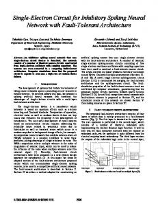
and-fire dynamics, in which the voltage on a single neuron increases linearly with time until a specified threshold is reached [8]. At this point the neuron suddenly fires by emitting an action potential and the neuronal voltage quickly returns to a reference level (Fig. 1). For concreteness and without loss of generality, we assume the rate of voltage increase and the threshold voltage are both equal to 1. We also assume that V is instantaneously set to zero after firing, i. e., we neglect delays in signal transmission between neurons [9].

I. INTRODUCTION

Networks of neurons which undergo “spiky” dynamics have been thoroughly investigated (see e.g. [1,2] and references therein). Nevertheless, a theory which describes the dynamics of randomly interconnected excitatory and inhibitory spiking neurons is still lacking. Even a system composed exclusively of inhibitory neurons [3–7] appears too complicated for analytical approaches. Part of the reason for this is that the dynamics of a single neuron involves many physiological features across a wide range of time scales that are difficult to incorporate into an analytical theory. Our goal in this work is to describe some of the dynamical features of a purely inhibitory neural network within the framework of a minimalist model. While we sacrifice realism by this approach, our model is analytically tractable. This feature offers the possibility that more realistic networks may be treated by natural extensions of our general framework. We specifically investigate an integrate-and-fire neural network, in which the integration step is purely linear in time, and in which there exists only inhibitory and instantaneous coupling between interacting neurons. We thus ignore potentially important features such as voltage leakage during the integration, as well as heterogeneity in the external drive and in the network couplings. However, we do not assume all-to-all coupling, an unrealistic construction which is often invoked as a simplifying assumption. Instead, the (average) number of “neighbors” is a basic parameter of our model. Analytically, we consider annealed coupling, where the neighbors of a neuron are reassigned after each neuron firing event. However, our simulations indicate that the model with quenched coupling, where the neighbors of each neuron are fixed for all time, gives nearly identical results. Each integrate-and-fire neuron is represented by a single variable – the polarization level, or voltage V . Our model has two fundamental ingredients: (i) the dynamics of individual neurons, and (ii) the interaction between them. For the former, we employ deterministic integrate-

Vi

i t

Vj

j

∆ t

FIG. 1. Illustration of the model dynamics. A single neuron i undergoes deterministic integrate-and-fire dynamics (upper right). When this neuron fires, its voltage Vi is set to zero, while simultaneously the voltages on all its inhibitory-coupled neighbors are reduced by ∆ (lower right).

The meaning of the inhibition is illustrated in Fig. 1. When a given neuron fires, it instantaneously transmits an inhibitory action potential to K randomly-chosen neighbors whose voltages are each reduced by an amount ∆. This inhibition delays the time until these inhibited neurons can reach threshold and ultimately fire themselves. The neighbors of a given neuron are selected at random from among all the neurons in the network and they are chosen anew every time any neuron fires. Thus 1

the coupling in the network is annealed. While a network with fixed quenched coupling is biologically much more realistic, annealed coupling means that a rate equation provides the exact description of the dynamics. Fortunately, the annealed and quenched systems appear to be statistically identical when the number of inhibitorycoupled neurons is sufficiently large. We shall consider only this limit in what follows. Within the rate equation approach, the distribution of neuronal voltages in our inhibitory network is described by linear dynamics except at the isolated times when a neuron fires. The underlying rate equation admits a steady state voltage distribution whose basic properties are established analytically in Sec. II. In general, although the network has a steady response, the dynamics of an individual neuron has an interesting history between firing events. We study, in particular, the probability that a neuron “survives” up to a time t after its last firing event in Sec. III. The survival probability decays exponentially in time with a decay rate that depends on the competition between the integration and the inhibitory coupling. This provides a relatively complete picture of the dynamics of a single neuron in the network. A summary is given in Sec. IV and some identities are proven in the Appendix.

P(s) =

1

dV P (V ) esV ,

(3)

−∞

to give, after some straightforward steps, P(s) =

K

es − 1 . − 1) + s/P1

(4)

(e−s∆

The unconventional definition of the Laplace transform reflects that fact that the voltage is restricted to lie in the range [−∞, 1]. To solve for the Laplace transform, we first note that P(0) = 1 due to normalization. Combining this with Eq. (4), we obtain P1 = (1 + K∆)−1 thus completing the solution. The final result is P(s) =

es − 1 . K (e−s∆ − 1) + s(1 + K∆)

(5)

It may be verified by elementary means that this function has a simple pole at s = −λ, that is, P(s) = A/(s + λ) + . . ., where λ is the root of
K eλ∆ − 1 − λ(1 + K∆) = 0, (6)

and A = (1 − e−λ )/[∆(1 + K∆)λ − 1]. The existence of a simple pole in the Laplace transform implies that the voltage distribution itself has an exponential asymptotic tail as V → −∞,

II. RATE EQUATIONS AND THE STEADY STATE

P (V ) → AeλV .

For the rate equation description we assume that the number of neurons is large and thus a continuum approach is appropriate. We define P (V, t)dV as the fraction of neurons whose voltage lies in the interval (V, V + dV ). Then the probability density P (V, t) obeys the master equation,   ∂ ∂ P (V, t) = P1 (t) δ(V ) (1) + ∂t ∂V + KP1 (t) [P (V + ∆, t) − P (V, t)] ,

(7)

The limiting behaviors of the decay constant λ may also be found from Eq. (6) and give    ∆−1 ln (K∆−1 ) when ∆ → 0, λ→ (8) 2(K∆2 )−1 when ∆ → ∞. 1.5

where P1 (t) ≡ P (V = 1, t). The second term on left-hand side accounts for the voltage increase because of the deterministic integration. The first term on the right-hand side accounts for the increase of zero-voltage neurons due to the firing of other neurons which have reached the threshold value Vmax = 1. The second set of terms accounts for the change in P (V ) due to the processes where V + ∆ → V and V → V − ∆ (we assume ∆ > 0 since inhibitory neurons are being considered). In the steady state, Eq. (1) simplifies to dP (V ) = P1 δ(V ) + KP1 [P (V + ∆) − P (V )] . dV

Z

P(V)

1.0

0.5

0.0 −0.5

0

0.5

1

V

(2)

FIG. 2. Typical simulation results for the steady state neuronal voltage distribution for a network of 25000 neurons, with annealed coupling to K = 50 other neurons and ∆ = 1/50. The distribution is shown at 10 time steps.

Equation (2) may be easily solved by introducing the Laplace transform, 2

To visualize these results, we have performed Monte Carlo simulations of an inhibitory neural network whose dynamics is defined by Eq. (1). A representative result is shown in Fig. 2 initial voltages uniformly distributed in [0, 1]. Essentially identical results are obtained for quenched inter-neuron coupling but all other system parameters unchanged. After approximately one time unit, the system has reached the steady state shown in the figure. Other initial conditions merely have different time delays until the steady state is reached. In addition to the exponential decay of the distribution for the smallest voltages, there are several other noteworthy features. First, there is a linear decay of the distribution to its limiting value P1 = (1 + K∆)−1 as V → 1 from below; this is reflective of the absorbing boundary condition at V = 1. There is also a sharp peak at V = 0, corresponding to the continuous input of reset neurons. For small ∆, almost all voltages lie within the range [0, 1]. This feature is reminiscent of the Bak-Sneppen evolution model [10] in which the “fitnesses” of most species lie within a finite target range, together with a small population of sub-threshold species. Finally we note that Eq. (1) applies even when the number of neighbors for a given neuron is not fixed. In this case, K may be interpreted as just the average number of interacting neighbors of a given neuron. Therefore K can be any positive real number. The voltage offset ∆ can also be heterogeneous, e. g., distributed in a finite range with some density ρ(∆). With this generalization, the term P (V + ∆) in Eq. (2) should be replaced R by d∆ ρ(∆)P (V + ∆). The resulting equation is still solvable by the same Laplace transform technique as in the homogeneous network and we now obtain a similar −1 solution to that R in Eq. (5) but with P1 = (1 + Kh∆i) , where h∆i = d∆ ρ(∆) ∆.

tually fire and why the survival probability decays exponentially at long times. In the absence of interactions, the voltage of a neuron increases deterministically with rate 1. On the other hand, inhibitory spikes, each of which reduce the voltage by ∆, occur stochastically with rate r = KP1 = K/(1 + K∆). This gives r∆ = K∆/(1 + K∆) < 1 for the rate at which the voltage decreases due to inhibition. Thus, on average the voltage increases at a net rate 1 − r∆ = (1 + K∆)−1 . Consequently the voltage of a tagged neuron must eventually reach the threshold and fire.

V 1

t1

t2

t3

t

FIG. 3. Voltage trajectory of a typical neuron following a voltage reset. Because each inhibitory spike reduces the voltage by ∆, a neuron which receives k inputs fires exactly at time τ = 1 + k∆. The horizontal tick marks are at t = 1, 1 + ∆, 1 + 2∆, and 1 + 3∆.

S(t) 1

S1(t)=1-e

-r

S2(t) S3(t)

III. EVOLUTION OF A SINGLE NEURON

1 In addition to the steady-state voltage distribution P (V ), we study the time dependence of an individual “tagged” neuron in the steady state. Consider, for example, a neuron which last fired at time T0 which we set to 0 for simplicity. The fate of this neuron may be generally characterized by its survival probability S(t), defined as the probability that this neuron has not yet fired again during the time interval (T0 , T0 + t), irrespective of how many inhibitory inputs it may have received (Fig. 3). A more comprehensive description is provided by Qk (t), the probability that the tagged neuron has not yet fired and that it received k inhibitory inputs during P (0, t). Clearly, S(t) = k≥0 Qk (t). As we now show, the survival probability and Qk (t) exhibit non-trivial firstpassage characteristics. Before discussing the survival probability in detail, let us first understand why a tagged neuron must even-

1+∆

1+2∆ 1+3∆

t

FIG. 4. Behavior of the survival probability as a function of time. This function is constant within each interval [1+(k−1)∆, 1+k∆] but exhibits an overall exponential decay in time.

From the above argument, the mean lifetime hti of a neuron between firing events is just the inverse of this rate. Thus hti = 1 + K∆.

(9)

Notice that the density of neurons which are firing, P1 , equals the inverse lifetime, as expected naively. Since the evolution of the neuronal voltage is a random-walk-like process which is biased towards an absorbing boundary in a semi-infinite geometry, the neuron survival probability must decay exponentially with time [11], 3

S(t) ∝ e−t/τ

when t → ∞.

k ≥ 2, the first spike must occur within [0, 1], while the remaining (time-ordered) k−1 spikes can occur anywhere within [t1 , t]. To evaluate the integral in Eq. (12), we may first integrate over t2 , . . . , tk . This integral is Z t Z t Z t dt2 dtk . (14) dt3 · · ·

(10)

To understand the asymptotic behavior of S(t), it is helpful to consider first the voltage evolution of a single neuron which has experienced 0, 1, 2, . . . inhibitory spikes. It is important to appreciate that a neuron which receives exactly k spikes necessarily fires exactly at time 1 + k∆ (Fig. 3). Thus the survival probability is a piecewise constant function which changes discontinuously at tk = 1 + k∆, k = 0, 1, 2, . . .. We now determine the value of S(t) at each of these plateaux. When t < 1, the tagged neuron has no possibility of firing and S(t) ≡ S0 = 1. To survive until time t = 1 + ∆, the neuron must receive at least one spike in the time interval [0, 1]. Since neurons experience spikes at constant rate r = KP1 , the probability of the neuron receiving no spikes in [0, 1] is e−r . The survival probability for 1 < t < 1 + ∆ thus equals S(t) ≡ S1 = 1 − e−r (Fig. 4). Similarly, to survive until time 1 + 2∆, the neuron must receive one spike before t = 1 and a second spike before t = 1 + ∆. By writing the probabilities for each of these events, we find, after straightforward steps, S2 = 1 − e−r − r e−r(1+∆) ,

t1

The domain of the integral is a simplex of size t − t1 and the integral is just (t − t1 )k−1 /(k − 1)!. Finally, we integrate over the region 0 < t1 < 1 to obtain

dtj .

k

Qk (t) = r e

−rt

Z

m (t − tm )k−m Y dtj . (k − m)! j=1

(16)

In particular, for k = m, we may write Qm (t) as rm e−rt Tm (∆), where

(12)

Tm (∆) =

Z

1

dt1

0

j=1

Z

1+∆

t1

dt2 . . .

Z

1+(m−1)∆

dtm .

(17)

tm−1

Remarkably, this expression has the simple closed-form representation (see Appendix)

Here the step function θ(1 + k∆ − t) guarantees that the voltage of the tagged neuron is below the threshold at time t. We must also ensure that the voltage is less than one throughout the entire time interval (0, t). The necessary and sufficient condition for this to occur is that the voltage is below threshold at each spike event. This determines the integration range in Eq. (12) to be tj−1 < tj < min[t, 1 + (j − 1)∆]

(15)

This expression actually holds for all k ≥ 0. From Eq. (15), we then find that S1 = 1 − e−r in the time range 1 < t < 1 + ∆. Generally in the time range 1+(m−1)∆ < t < 1+m∆, a tagged neuron which has not fired must have experienced at least m spikes; therefore Qk = 0 for k < m. To determine the non-zero Qk ’s – those with k ≥ m – note that the first m spikes must obey the constraint of Eq. (13), while each of the remaining k − m spikes may lie anywhere within the time interval tm and t. The latter condition again defines a simplex of size t − tm . This gives the contribution (t − tm )k−m /(k − m)! for the integral over these variables. By this reduction, the k-fold integral in Eq. (12) collapses to the m-fold integral

This direct approach becomes increasingly unwieldy for large times, however, and we now present a more systematic approach. To this end, we first solve for Qk (t), the probability that the tagged neuron has experienced k inhibitory inputs but has not yet fired. For a constant rate r of inhibitory spikes, the probability that the tagged neuron has been spiked exactly k times, with each spike occurring in the Q time intervals [tj , tj + dtj ], j = 1, 2, . . . , k, equals e−rt 1≤j≤k r dtj . Therefore, Z Y k

(rt)k − (rt − r)k −rt e . k!

Qk (t) =

1 + ∆ < t < 1 + 2∆. (11)

Qk (t) = rk e−rt θ(1 + k∆ − t)

tk−1

t2

(1 + m∆)m−1 m!

(18)

rm (1 + m∆)m−1 −rt e . m!

(19)

Tm (∆) = so that Qm (t) =

(13)

for j = 1, . . . , k (we set t0 ≡ 0). We now evaluate Qk (t) successively for each time window [1 + (j − 1)∆, 1 + j∆]. Consider first the range 1 < t < 1 + ∆. Here a tagged neuron which has not fired must have received at least one spike. Consequently Q0 (t) = 0. Similarly, if a neuron receives a single spike and survives until t = 1 + ∆, the spike must have occurred in the time range [0, 1]. Hence Q1 = re−rt . For

For large m and also fork > m, the explicit expressions for Qk become quite cumbersome; however, they are not needed to determine the asymptotics of the survival probability. We now use our result for Qk to determine the survival probability. For the time rangeP [1+(m−1)∆, 1+m∆], we substitute Eq. (16) in S(t) = k≥m Qk (t) and perform the sum over k to give 4

Sm = r

m

Z

e−rtm

m Y

dtj .

K → ∞,

(20)

This neat expression formally shows that the survival probability is constant but m dependent inside the time interval [1 + (m − 1)∆, 1 + m∆]. These properties justify the notation in Eq. (20). The integral on the right-hand side of Eq. (20) can be simplified by integrating over tm to give

Sm ∝ rm Tm e−r(1+m∆).

Sm = 1 −

(21)

τ =−

rn Tn e−r(1+n∆) .

Since S∞ = 0, we rewrite this as ∞ X

rn Tn e−r(1+n∆)

(22)

n=m

which is more convenient for determining asymptotic behavior. Let us first use this survival probability to compute the average time interval hti between consecutive firings of the same neuron. This is  Z ∞  dS t − hti = dt dt Z0 ∞ = S(t) dt 0 X =1+∆ Sm m≥1

=1+∆

X

n rn Tn e−r(1+n∆) .

∆ . P1 + ln(1 − P1 )

(26)

The different behavior of the two basic time scales, τ and hti = 1/P1 , is characteristic of biased diffusion near an absorbing boundary in one dimension [11]. Here, the mean survival time is simply the distance from the particle to the absorbing boundary divided by the mean velocity v. In contrast, the survival probability asymptotically decays as exp(−v 2 t/D), so that τ = D/v 2 , independent of initial distance. It is instructive to interpret these results for our neural network, where a single neuron can be viewed as undergoing a random walk in voltage, with a step to smaller voltage of magnitude ∆ occurring with probability r dt in a time interval dt and a step to larger voltage of magnitude dt occurring with probability 1 − r dt. For this random walk, the bias velocity is v = 1 − r∆ = (1 + K∆)−1 = P1 . This then reproduces hti = 1/v = 1+K∆ = 1/P1 . Moreover, the diffusion coefficient of this random walk is simply D ∝ r∆2 . This random walk description should be valid when K∆ ≈ 1/P1 ≫ 1 or r∆ → 1, so that a tagged neuron experiences many spikes between firing events. This then leads to τ = D/v 2 ∝ K 2 ∆3 . In this diffusive limit of P1 → 0, the limiting behavior of Eq. (26) agrees with this expression for τ .

n=0

Sm =

(25)

Using Eqs. (25), (18), and Stirling’s formula, we deduce that S(t) decays exponentially with time, with the relaxation time in Eq. (10) given by

This recursion relation allows us to express the survival probability in terms of the Tn ’s with n < m: m−1 X

K∆ = O(1)

appears biologically relevant. In this limit and when the time t = 1 + m∆ is large, the series for Sm in Eq. (22) is geometric. Hence, apart from a prefactor, the survival probability is given by the first term in this series:

j=1

Sm = Sm−1 − rm−1 Tm−1 e−r[1+(m−1)∆].

∆ → 0,

(23)

n≥1

In the first line, we use the fact that −S˙ is just the probability that the neuron fires at a time t after its previous firing, and the last line was derived by employing Eq. (22). As discussed previously, the average time between firings of the same neuron is hti = 1 + K∆. Equation (23) agrees with this iff the identity X

n≥0

nTn z n =

r er 1 − r∆

with z ≡ r e−r∆

IV. SUMMARY

We have determined the dynamical behavior of an integrate-and-fire neural network in which there is purely inhibitory annealed coupling between neighboring neurons. The same behavior is also exhibited by a model with quenched coupling. Our model should be regarding as a “toy”, since so many realistic physiological features have been neglected. However, this toy model has the advantage of being analytically tractable. We have determined both the steady state properties of the network, as well as the complete time-dependent behavior of a single neuron. The latter gives rise to an appealing first-passage problem for the probability for a neuron to survive a time t after its last firing. This survival probability is piecewise constant but with an overall exponential decay in time.

(24)

holds. This is also verified in Appendix. Let us now interpret our results in the context of biological applications. Typically, the number of neighboring neurons K is large while the spike-induced voltage decrement ∆ of a neuron is small, so that the total voltage decrease K∆ is of order one. In other words, the limit 5

I dz r er 1 2πi 1 − r∆ z n+1 I r er z ′ (r) 1 dr = 2πi (1 − r∆)[z(r)]n+1 I r(1+n∆) 1 e = dr 2πi rn (1 + n∆)n−1 = . (n − 1)!

Given the simplicity of the model, it should be possible to incorporate some of the more important features of real inhibitory neural networks, such as neurons with leaky voltages and finite propagation velocity for inhibitory signals, into the rate equation description. These generalizations may provide a tractable starting point to investigate more complex dynamical behavior which are often the focus of neural network studies, such as largescale oscillations and macroscopic synchronization.

nTn =

We thank C. Borgers, S. Epstein, N. Kopell, and S. Yeung for stimulating discussions. We are also grateful to NSF grant No. DMR9978902 for partial financial support. APPENDIX A: BASIC IDENTITIES

[1] N. Brunel, J. Comput. Neurosci. 8, 183–208 (2000). [2] D. Golomb and D. Hansel, Neural Comput. 12, 1095– 1139 (2000). [3] C. van Vreeswijk and L. F. Abbott, SIAM J. Appl. Math. 53, 253-264 (1993). [4] D. Golomb and J. Rinzel, Phys. Rev. E 48, 4810–4814 (1993); Physica D 72, 259-282 (1994). [5] X.-J. Wang and G. Buzs´ aki, J. Neurosci. 16, 6402–6413 (1996). [6] J. A. White, C. C. Chow, J. Ritt, C. Soto-Trevino, and N. Kopell, J. Comput. Neurosci. 5, 5–16 (1998). [7] N. Brunel and V. Hakim, Neural Comput. 11, 1621–1671 (1999). neurons with low firing rates.” [8] This model was introduced in J. Lapicque, J. Physiol. (Paris) 9, 620–635 (1907). See H. C. Tuckwell, Introduction to theoretical neurobiology, Vol. 1 (Cambridge University Press, Cambridge, 1988) for a general introduction. [9] See e.g. Y. Nakamura, F. Tominaga, and T. Munakata, Phys. Rev. E 49, 4849–4856 (1994); U. Ernst, K. Pawelzik, and T. Geisel, ibid. 57, 2150–2162 (1998); E. M. Izhikevich, ibid. 58, 905–908 (1998); M. K. S. Yeung and S. H. Strogatz, Phys. Rev. Lett. 82, 648–651 (1999). [10] P. Bak and K. Sneppen, Phys. Rev. Lett. 71, 4083–4086 (1993). [11] S. Redner, A guide to first-passage processes (Cambridge University Press, New York, 2001).

We use Eq. (22) to derive the identity (18). First, we note that S0 = 1. By substituting this into Eq. (22) we obtain X Tn z n = er with z ≡ r e−r∆ . (A1) n≥0

The requirement that Eq. (A1) holds for arbitrary r and ∆ leads to unique set of Tn ’s. To determine these Tn ’s, let us treat z as a complex variable. Then employing the Cauchy formula yields I er 1 dz Tn = n+1 2πi z I 1 er z ′ (r) = dr 2πi [z(r)]n+1 I (1 − r∆) er(1+n∆) 1 dr = 2πi rn+1 (1 + n∆)n (1 + n∆)n−1 = −∆ n! (n − 1)! (1 + n∆)n−1 . = n! Next we verify Eq. (24) by repeating the procedure which has just been used to check Eq. (A1). As above, the quantity nTn may be written in the integral representation

6